hep-ph/0001129 FTUV/00-04 IFIC/00-04
Neutrino Masses and Mixing one Decade from Now

Abstract

We review the status of neutrino masses and mixings in the light of the solar and atmospheric neutrino data. The result from the LSND experiment is also considered. We discuss the present knowledge and the expected sensitivity to the neutrino mixing parameters in the simplest schemes proposed to reconcile these data some of which include a light sterile neutrino in addition to the three standard ones.

1 Indications for Neutrino Mass: Two–Neutrino Analysis

Neutrinos are the only massless fermions predicted by the Standard Model. This seemed to be a reasonable assumption as none of the laboratory experiments designed to measure the neutrino mass have found any positive evidence for a non-zero neutrino mass. However, the confidence on the masslessness of the neutrino is now under question due to the important results of underground experiments, starting by the geochemical experiments of Davis and collaborators till the more recent Gallex, Sage, Kamiokande and Super–Kamiokande (SK) experiments solarexp ; atmexp ; sk99 . Altogether they provide solid evidence for the existence of anomalies in the solar and the atmospheric neutrino fluxes which could be explained by the hypothesis of neutrino oscillations which requires the presence of neutrino masses and mixings. Particularly relevant has been the recent confirmation by the SK collaboration sk99 of the atmospheric neutrino zenith-angle-dependent deficit which strongly indicates towards the existence of $\nu_{\mu}$ conversion. Together with these results there is also the indication for neutrino oscillations in the $\bar{\nu}_{\mu}\rightarrow\bar{\nu}_{e}$ channel by the LSND experiment lsnd .

We first review our present knowledge of the present experimental status for the different evidences and present the results of the different analysis in the framework of two–neutrino oscillations.

1.1 Solar Neutrinos

At the moment, evidence for a solar neutrino deficit comes from five experiments solarexp : Homestake, Kamiokande, SK and the radiochemical Gallex and Sage experiments. The most recent data on the rates can be summarized as:

Clorine $$2.56\pm 0.23\;\;\mbox{SNU}$$

Gallex and Sage $$72.2\pm 5.6\;\;\mbox{SNU}$$

Super–Kamiokande $$(2.45\pm 0.08)\times 10^{6}\;\;\mbox{cm${}^{-2}$s${}^{-1}$}$$

Super-Kamiokande has also measured the the time dependence of the event rates during the day and night, as well as a measurement of the recoil electron energy spectrum and has also presented preliminary results on the seasonal variation of the neutrino event rates, an issue which will become important in discriminating the MSW scenario from the possibility of neutrino oscillations in vacuum.

The different experiments are sensitive to different parts of the energy spectrum of solar neutrinos and putting all these results together seems to indicate that the solution to the problem is not astrophysical but must concern the neutrino properties. Moreover, non-standard astrophysical solutions are strongly constrained by helioseismology studies Bahcall98 . Within the standard solar model approach, the theoretical predictions clearly lie far from the best-fit solution what leads us to conclude that new particle physics is the only way to account for the data.

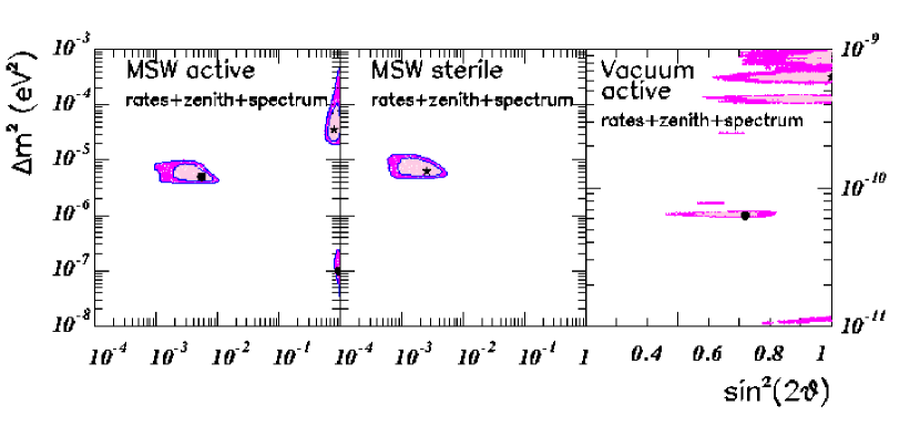
Figure 1: Presently allowed solar neutrino parameters for two-neutrino oscillations by the global analysis from Ref. oursun ; ourfour . The plotted regions are 90% (lighter) and 99% CL (darker).

The standard explanation for this deficit is the oscillation of $\nu_{e}$ to another neutrino species either active or sterile. In Fig. 1 we show the allowed two-neutrino oscillation regions obtained in our updated global analysis of the solar neutrino data oursun ; ourfour for both MSW msw as well as vacuum oscillations vacuum into active or sterile neutrinos. These results indicate that for oscillations into active neutrinos there are four possible solutions for the parameters:

• vacuum (also called “just so”) oscillations with $\Delta m^{2}_{ei}=(0.5$–$8)\times 10^{-10}$ eV² and $\sin^{2}(2\theta)=0.5$–$1$

• non-adiabatic-matter-enhanced oscillations (SMA) via the MSW mechanism with $\Delta m^{2}_{ei}=(0.4$–$1)\times 10^{-5}$ eV² and $\sin^{2}(2\theta)=(1$–$10)\times 10^{-3}$, and

• large mixing (LMA) via the MSW mechanism with $\Delta m^{2}_{ei}=(0.2$–$5)\times 10^{-4}$ eV² and $\sin^{2}(2\theta)=0.6$–$1$.

• low mass solution (LOW) via the MSW mechanism with $\Delta m^{2}_{ei}=(0.5$–$2)\times 10^{-7}$ eV² and $\sin^{2}(2\theta)=0.8$–$1$.

For oscillations into an sterile neutrino there are differences partly due to the fact that now the survival probability depends both on the electron and neutron density in the Sun but mainly due to the lack of neutral current contribution to the water cerencov experiments. Unlike active neutrinos which lead to events in the Kamiokande and SK detectors by interacting via neutral current with the electrons, sterile neutrinos do not contribute to the SK event rates. Therefore a larger survival probability for ${}^{8}B$ neutrinos is needed to accommodate the measured rate. As a consequence a larger contribution from ${}^{8}B$ neutrinos to the Chlorine and Gallium experiments is expected, so that the small measured rate in Chlorine can only be accommodated if no ${}^{7}Be$ neutrinos are present in the flux. This is only possible in the SMA solution region, since in the LMA and LOW regions the suppression of ${}^{7}Be$ neutrinos is not enough. Vacuum oscillations into sterile neutrinos are also ruled out with more than 99% CL.

1.2 Atmospheric Neutrinos

Atmospheric showers are initiated when primary cosmic rays hit the Earth’s atmosphere. Secondary mesons produced in this collision, mostly pions and kaons, decay and give rise to electron and muon neutrino and anti-neutrinos fluxes. There has been a long-standing anomaly between the predicted and observed $\nu_{\mu}$ $/\nu_{e}$ ratio of the atmospheric neutrino fluxes atmexp . Although the absolute individual $\nu_{\mu}$ or $\nu_{e}$ fluxes are only known to within $30\%$ accuracy, different authors agree that the $\nu_{\mu}$ $/\nu_{e}$ ratio is accurate up to a $5\%$ precision. In this resides our confidence on the atmospheric neutrino anomaly (ANA), now strengthened by the high statistics sample collected at the SK experiment sk99 . The most important feature of the atmospheric neutrino data is that it exhibits a zenith-angle-dependent deficit of muon neutrinos which is inconsistent with expectations based on calculations of the atmospheric neutrino fluxes. This experiment has marked a turning point in the significance of the ANA.

The most likely solution of the ANA involves neutrino oscillations. In principle we can invoke various neutrino oscillation channels, involving the conversion of $\nu_{\mu}$ into either $\nu_{e}$ or $\nu_{\tau}$ (active-active transitions) or the oscillation of $\nu_{\mu}$ into a sterile neutrino $\nu_{s}$ (active-sterile transitions) atmours . Oscillations into electron neutrinos are nowadays ruled out since they cannot describe the measured angular dependence of muon-like contained events atmours . Moreover the most favoured range of masses and mixings for this channel have been excluded by the negative results from the CHOOZ reactor experiment chooz .

In Fig. 2 we show the allowed neutrino oscillation parameters obtained in a recent global fit of the full data set of atmospheric neutrino data on vertex contained events at IMB, Nusex, Frejus, Soudan, Kamiokande atmexp and SK experiments sk99 as well as upward going muon data from SK, Macro and Baksan experiments in the different oscillation channels.

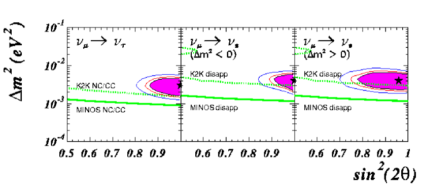
Figure 2: Allowed atmospheric oscillation parameters all for experiments, combined at 90 (shadowed area), 95 % and 99 % CL (thin solid line) for all possible oscillation channels, from Ref. atmnew . The expected sensitivity for upcoming long-baseline experiments is also displayed.

The two panels corresponding to oscillations into sterile neutrinos in Fig. 2 differ in the sign of the $\Delta m^{2}$ which was assumed in the analysis of the matter effects in the Earth for the $\nu_{\mu}\to\nu_{s}$ oscillations. Notice that in all channels where matter effects play a role the range of acceptable $\Delta m^{2}$ is shifted towards larger values, when compared with the $\nu_{\mu}\to\nu_{\tau}$ case. This follows from looking at the relation between mixing in vacuo and in matter. In fact, away from the resonance region, independently of the sign of the matter potential, there is a suppression of the mixing inside the Earth. As a result, there is a lower cut in the allowed $\Delta m^{2}$ value, and it lies higher than what is obtained in the data fit for the $\nu_{\mu}\to\nu_{\tau}$ channel.

Concerning the quality of the fits our results show that the best fit to the full sample is obtained for the $\nu_{\mu}\to\nu_{\tau}$ channel although from the global analysis oscillations into sterile neutrinos cannot be ruled out. This arises mainly from the fact that due to matter effects the distribution for upgoing muons in the case of $\nu_{\mu}\to\nu_{s}$ are flatter than for $\nu_{\mu}\to\nu_{\tau}$ lipari . Data show a somehow steeper angular dependence which can be better described by $\nu_{\mu}\to\nu_{\tau}$. This leads to the better quality of the global fit in this channel. Pushing further this feature Super-Kamiokande collaboration has presented a preliminary partial analysis of the angular dependence of the through-going muon data in combination with the up-down asymmetry of partially contained events which seems to exclude the possibility $\nu_{\mu}\to\nu_{s}$ at the 2–$\sigma$ level sk99 .

1.3 LSND

Los Alamos Meson Physics Facility (LSND) has searched for $\bar{\nu}_{\mu}\to\bar{\nu}_{e}$ oscillations with $\bar{\nu}_{\mu}$ from $\mu^{+}$ decay at rest lsnd . The $\bar{\nu}_{e}$’s are detected in the quasi elastic process $\bar{\nu}_{e}\,p\to e^{+}\,n$ in correlation with a monochromatic photon of $2.2$ MeV arising from the neutron capture reaction $np\to d\gamma$. In Ref. lsnd they report a total of 22 events with $e^{+}$ energy between 36 and $60$ MeV while $4.6\pm 0.6$ background events are expected. They fit the full $e^{+}$ event sample in the energy range $20<E_{e}<60$ MeV by a $\chi^{2}$ method and the result yields $64.3^{+18.5}_{-16.7}$ beam-related events. Subtracting the estimated neutrino background with a correlated gamma of $12.5\pm 2.9$ events results into an excess of $51.8^{+18.7}_{-16.9}\pm 8.0$ events. The interpretation of this anomaly in terms of $\bar{\nu}_{\mu}\to\bar{\nu}_{e}$ oscillations leads to an oscillation probability of ($0.31^{+0.11}_{-0.10}\pm 0.05$)%. Using a likelihood method they obtain a consistent result of ($0.27^{+0.12}_{-0.12}\pm 0.04$)%. In the two-family formalism this result leads to the oscillation parameters shown in Fig. 3. The shaded regions are the 90 % and 99 % likelihood regions from LSND. Also shown are the limits from BNL776, KARMEN1, Bugey, CCFR, and NOMAD.

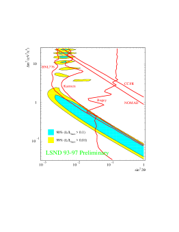
Figure 3: Allowed LSND oscillation parameters compared with the 90 % exclusion regions from other experiments.

2 $\nu$–Oscillation Searches at Reactor and Accelerator Experiments

There are two types of laboratory experiments to search for neutrino oscillations. In a disappearance experiment one looks for the attenuation of a neutrino beam primarily composed of a single flavour due to the mixing with other flavours. On the other hand in an appearance experiment one searches for interactions by neutrinos of a flavour not present in the neutrino beam. Several experiments have been searching for these signatures without any positive observation. Their results are generally presented as exclusion areas in the two-neutrino oscillation approximation. From these figures it is possible to obtain the limits obtained by the experiments on the corresponding transition probabilities. This is the relevant quantity when interpreting the sensitivities in the framework of more–than–two–neutrino mixing. In table 1 we show the limits on the different transition probabilities from the negative results of the most restricting short baseline experiments.

Table 1: 90% CL on the neutrino transition (or survival) probabilities from the negative searches at short baseline experiments

. Experiment Channel Limit (90%) $\Delta m^{2}_{min}$ (eV²) Reference CDHSW $\nu_{\mu}\rightarrow\nu_{\mu}$ $P_{\mu\mu}>0.95$ 0.25 CDHSW E776 $\nu_{\mu}\rightarrow\nu_{e}$ $P_{e\mu}<1.5\times 10^{-3}$ 0.075 E776 Karmen $\bar{\nu}_{\mu}\rightarrow\bar{\nu}_{e}$ $P_{e\mu}<7\times 10^{-4}$ 0.05 karmen E531 $\nu_{\mu}\rightarrow\nu_{\tau}$ $P_{\mu\tau}<0.02$ 1 E531 Chorus/Nomad $\nu_{\mu}\rightarrow\nu_{\tau}$ $P_{\mu\tau}<6.5\times 10^{-4}$ 0.9 chorus

Due to the short path length of the neutrino in this experiments they are not sensitive to the low values of $\Delta m^{2}$ invoked to explain both the solar and the atmospheric neutrino data.

For the determination of the neutrino mass matrix structure the most important short baseline experiment will be upcoming MiniBooNE miniboone experiment the first stage of the which is scheduled to start taking data in 2001. It searches for $\nu_{e}$ appearance in the Fermilab $\nu_{\mu}$ beam and it is specially designed to make a conclusive statement about the LSND’s neutrino oscillation evidence. In Fig. 4 we show the 90% CL limits that MiniBooNE can achieve. Should a sign be found then the next step would be the BooNe experiment.

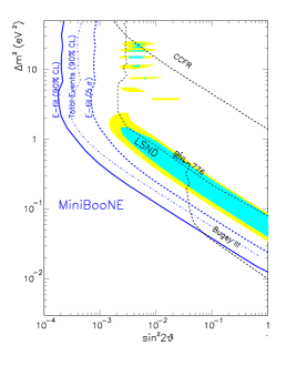
Figure 4: MiniBooNE 90 % CL limits using energy–dependent fit (solid) and total even counting (dot-dash). Also shown is the 5$\sigma$ sensitivity contour of the energy dependent fit (dashed).

Smaller values of $\Delta m^{2}$ can be accessed at reactor experiments due to the lower neutrino beam energy as well as future long baseline experiments due to the longer distance travelled by the neutrino. In table 2 we show the limits on the different transition probabilities from the negative results of the reactor experiments Bugey and CHOOZ as well as the expected sensitivities at future long baseline experiments both at accelerator and reactors.

Table 2: 90% CL on the neutrino transition (or survival) probabilities from the negative searches at short baseline experiments

. Experiment Type Channel Limit (90%) $\Delta m^{2}_{min}$ (eV²) Ref. Bugey Present Reactor $\nu_{e}\rightarrow\nu_{e}$ $P_{ee}>0.95$ $10^{-2}$ bugey CHOOZ Present Reactor $\nu_{e}\rightarrow\nu_{e}$ $P_{ee}>0.91$ $10^{-3}$ chooz Borexino LBL Reactor $\nu_{e}\rightarrow\nu_{e}$ $P_{ee}>0.9$ $10^{-6}$ borexino Kamland LBL Reactor $\nu_{e}\rightarrow\nu_{e}$ $P_{ee}>0.95$ $10^{-5}$ kamland K2K LBL NC/CC $\nu_{\mu}\rightarrow\nu_{\mu}$ $P_{\mu\mu}>0.77$ $1.5\times 10^{-3}$ k2k LBL Disapp $\nu_{\mu}\rightarrow\nu_{\mu}$ $P_{\mu\mu}>0.75$ $3\times 10^{-3}$ LBL Appea $\nu_{\mu}\rightarrow\nu_{e}$ $P_{\mu e}<0.04$ $10^{-3}$ MINOS LBL NC/CC $\nu_{\mu}\rightarrow\nu_{\mu}$ $P_{\mu\mu}>0.99$ $9\times 10^{-4}$ minos LBL Disapp $\nu_{\mu}\rightarrow\nu_{\mu}$ $P_{\mu\mu}>0.98$ $1.2\times 10^{-3}$ LBL Appea $\nu_{\mu}\rightarrow\nu_{e}$ $P_{\mu e}<1\times 10^{-3}$ $1\times 10^{-3}$

3 Three–Neutrino Oscillations

In the previous section we have discussed the evidences for neutrino masses and mixings as usually formulated in the two neutrino oscillation scenario. We want now to fit all the different evidences in a common framework and see what is our present knowledge of the neutrino mixing and masses and how this may be improved by the upcoming experiments. In doing so it is of crucial relevance the confirmation or reprobation of the LSND result by the MiniBooNE experiment. The three evidences can be interpreted in terms of neutrino oscillations but with the need of three different mass scales. Thus if the LSND is ruled out by the MiniBooNE experiment we could fit both solar and atmospheric data in terms of three–neutrino oscillations. If, on the contrary, LSND result stands the test of time, this would be a puzzling indication for the existence of a light sterile neutrino and the need to work in a four–neutrino framework.

In the first case, i.e. three–neutrino framework, the evolution equation for the three neutrino flavours can be written as:

$$-i\frac{d\nu}{dt}=\left[U\frac{M_{\nu}}{2E}U^{\dagger}+H_{int}\right]\;,$$ (1)

where $M_{\nu}$ is the diagonal mass matrix for the three neutrinos and $U$ is the unitary matrix relating the flavour and the mass basis. $H_{int}$ is the Hamiltonian describing the neutrino interactions. In general $U$ contains 3 mixing angles and 1 or 3 CP violating phases depending on whether the neutrinos are Dirac or Majorana (For a detail discussion see Ref.Pilar ) . Here we will neglect the CP violating phases as they are not accessible by the existing experiments. We define the unitary matrix as

$$U=R_{23}(\theta_{23})\times R_{13}(\theta_{13})\times R_{12}(\theta_{12})\;,$$ (2)

where $R_{ij}$ is a rotation matrix in the plane $ij$.

In this framework a neutrino of definite flavour $\nu_{\alpha}$, after travelling a distance $L$ in vacuum, can be detected in the charged-current (CC) interaction $\nu\;N^{\prime}\rightarrow l_{\beta}\;N$ with a probability

$$P_{\alpha\beta}=\delta_{\alpha\beta}-4\sum_{i=1}^{n}\sum_{j=i+1}^{n}\mbox{Re}[U_{\alpha i}U^{\star}_{\beta i}U^{\star}_{\alpha j}U_{\beta j}]\sin^{2}\left(\frac{\Delta_{ij}}{2}\right)\;.$$ (3)

The probability, therefore, oscillates with oscillation lengths $\Delta_{ij}$ given by

$$\frac{\Delta_{ij}}{2}=1.27\frac{|m_{i}^{2}-m_{j}^{2}|}{\mbox{eV}^{2}}\frac{L/E}{\mbox{m/MeV}}=1.27\frac{\Delta m^{2}_{ij}}{\mbox{eV}^{2}}\frac{L/E}{\mbox{m/MeV}}\;,$$ (4)

where $E$ is the neutrino energy.

In general the transition probabilities will present an oscillatory behaviour with two oscillation lengths. In order to explain the solar and atmospheric neutrino data we impose the lengths to be in the range such that:

$$\Delta m_{12}^{2}\simeq\Delta m^{2}_{solar}<10^{-4}\mbox{eV}^{2}\;,\;\;\;\;\;\;\;\;\;\;\;\;\Delta m_{23}^{2}\simeq\Delta m^{2}_{atm}\sim 10^{-3}\mbox{eV}^{2}\;.$$ (5)

In this way, for instance, the electron and muon neutrino survival probabilities in vacuum are given by

$$P_{ee} = 1-\cos^{4}\theta_{13}\sin^{2}(2\theta_{12})\sin^{2}\left(\frac{\Delta_{sol}}{2}\right)-\sin^{2}(2\theta_{13})\sin^{2}\left(\frac{\Delta_{atm}}{2}\right)\;,$$ (6)

$$P_{\mu\mu} = 1-\cos^{2}\theta_{13}\sin^{2}\theta_{23}(1-\cos^{2}\theta_{13}\sin^{2}\theta_{23})\sin^{2}\left(\frac{\Delta_{atm}}{2}\right)$$

$$-4(\sin\theta_{12}\cos\theta_{23}-\cos\theta_{12}\sin\theta_{13}\sin\theta_{23})^{2}$$

$$(\cos\theta_{12}\sin\theta_{23}+\sin\theta_{12}\sin\theta_{13}\sin\theta_{23})^{2}\sin^{2}\left(\frac{\Delta_{sol}}{2}\right)\;.$$

For the physically interesting case $\Delta m^{2}_{solar}\ll\Delta m^{2}_{atm}$ we find that the solar and atmospheric neutrino oscillations decouple in the limit $\theta_{13}=0$. In this case the values of the mixing angles $\theta_{12}$ and $\theta_{23}$ can be obtained directly from the results of the analysis in terms of two–neutrino oscillations presented in the first section. Although for simplicity we have restricted here to vacuum oscillations, the decoupling is still valid in the presence of matter.

Deviations from the two–neutrino scenario are then determined by the size of the mixing angle $\theta_{13}$. The first question to answer is how the presence of this new angle affects our analysis of the solar and atmospheric neutrino data. For vacuum solution to the solar neutrino problem the answer is simply given in Eq. (6). For the case of MSW solutions it has been shown (see Ref.fogli ) that

$$P^{3\nu}_{ee,MSW}=\sin^{4}(\theta_{13})+\cos^{4}(\theta_{13})P^{2\nu}_{ee,MSW}$$ (8)

where $P^{2\nu}_{ee,MSW}$ is obtained with the modified sun density $N_{e}\rightarrow\cos^{2}(\theta_{13})N_{e}$. In Fig. 5 we show the allowed regions for the oscillation parameters $\Delta m_{12}$ and $\sin^{2}(\theta_{12})$ from the analysis of the solar neutrino experiments event rates in the framework of three–neutrino oscillations for different values of the angle $\theta_{13}$.

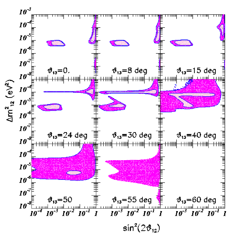
Figure 5: Allowed regions at 90% and 99% CL for the oscillation parameters $\Delta m_{12}$ and $\sin^{2}(\theta_{12})$ from the analysis of the solar neutrino experiments event rates in the framework of three–neutrino oscillations for different values of the angle $\theta_{13}$.

As seen in the figure the effect is small unless very large values of $\theta_{13}$ are involved. In particular for $\sin^{2}(\theta_{13})<0.2$ ($\theta_{13}<25^{\circ}$) there are still two separated SMA and LMA solutions in the ($\Delta m^{2}_{12}$,$\sin^{2}(\theta_{12})$ ) plane (see also Fogli’s talk and reference therein).

For a detail study of the effect of $\theta_{13}$ in the analysis of the atmospheric neutrino data we refer to Fogli’s talk in these proceedings. The conclusion is that for the presently allowed values of $\theta_{13}$ by the CHOOZ experiment (see below) the two–flavour analysis of the solar and atmospheric neutrino data are good approximations in the determination of the allowed mass splitings $\Delta m_{12}^{2}$ and $\Delta m^{2}_{23}$ and mixing angles $\theta_{12}$ and $\theta_{23}$.

We must now turn to our present knowledge of the value of the mixing angle $\theta_{13}$. Short baseline experiments cannot provide any information on the value of this angle, as they are not sensitive to oscillations since for both mass splitings the oscillating phase is too small. On the other hand experiments at reactor and long baseline experiments can be sensitive to oscillations with $\Delta m^{2}_{23}$ . In Table 3 we show the expression for the transition probabilities relevant for each of the experiments in the three–neutrino framework.

Experiment	Probability	Sensitivity
Reactor	$P_{ee}=1-4s^{2}_{13}c^{2}_{13}S^{2}_{atm}$	Good
LBL at Acc	$P_{\mu\mu}=1-4c^{2}_{13}s^{2}_{23}(1-c^{2}_{13}s^{2}_{23})S^{2}_{atm}$	Bad
	$P_{e\mu}=4s^{2}_{13}c^{2}_{13}s^{2}_{23}S^{2}_{atm}$	Good

In Table 3 $s_{i}=\sin(\theta_{i})$ and $c_{i}=\cos(\theta_{i})$ and $S^{2}_{atm}=\langle\sin^{2}\left(\frac{\Delta_{23}}{2}\right)\rangle$.

Long baseline experiments at reactors such as Borexino and Kamland due to the long baseline and lower reactor neutrino energy can be sensitive to both oscillation lengths

$$P_{ee}^{\mbox{LBL at reac}}=1-4s^{2}_{12}c^{2}_{12}c_{13}^{4}S^{2}_{sun}-4s^{2}_{13}c^{2}_{13}S^{2}_{atm}$$ (9)

In this case if the solution to the solar neutrino deficit is the SMA the contribution from the piece in $S^{2}_{sun}$ is very small and the experiments can be sensitive to $\theta_{13}$ by the observation of oscillations with the shorter wavelength. For the LMA solution to the solar neutrino problem, however, both terms can contribute and in consequence the precision attainable on $\theta_{13}$ depends on the precise knowledge of the solar neutrino parameters $\theta_{12}$ and $\delta m^{2}_{12}$ which would be achieved at future solar neutrino experiments such as SNO presently running at Sudbury and Borexino at Gran Sasso.

In Fig. 6 we plot the presently excluded region in the $\theta_{13}$ $\Delta m^{2}_{23}$ plane by the present reactor experiments as well as the attainable sensitivity at the future long baseline experiments listed in Table 2. One must, however, take these value as the “ultimate” sensitivity that could be achieved at these experiments. The results presented in Fig. 6 were obtained by direct translation of the usual two–neutrino exclusion regions to the tree–neutrino scenario. But the original exclusion regions where obtained assuming only two–neutrino oscillations for the corresponding channel while in the case of three–neutrino mixings there may be new sources of backgrounds arising from other channels what can worsen the sensitivity. In order to obtain the definite sensitivity in the angle $\theta_{13}$ the experiments should redo their analysis in the framework of three–neutrino oscillations.

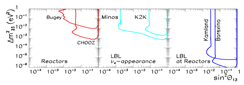
Figure 6: Presently excluded region in the $\theta_{13}$ $\Delta m^{2}_{23}$ plane at 90% CL by the reactor experiments as well as the attainable sensitivity at the future long baseline experiments. For the central panel the region is plotted for the values $\sin^{2}(2\theta_{23})>0.8$ favoured by the atmospheric neutrinos analysis. The regions plotted for the LBL experiments at reactors are obtained assuming the SMA solution for the solar neutrino problem.

4 Four-Neutrino Schemes

In the previous section we have discussed the neutrino mixing parameters assuming that the LSND result would be not confirmed by the MiniBooNE experiment. If the opposite holds then the simplest way to open the possibility of incorporating the LSND results to the solar and atmospheric neutrino evidences is to invoke a sterile neutrino, i.e. one whose interaction with standard model particles is much weaker than the SM weak interaction so it does not affect the invisible Z decay width, precisely measured at LEP. The sterile neutrino must also be light enough in order to participate in the oscillations involving the three active neutrinos.

After imposing the present constrains from the negative searches at accelerator and reactor neutrino oscillation experiments one is left with two possible mass patterns as described in Fig. 7 which we will call scenario I and II.

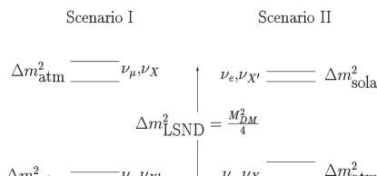
Figure 7: Allowed scenarios for four–neutrino oscillations.

In scenario I there are two lighter neutrinos at the solar neutrino mass scale and two maximally mixed almost degenerate eV-mass neutrinos split by the atmospheric neutrino scale. In scenario II the two lighter neutrinos are maximally mixed and split by the atmospheric neutrino scale while the two heavier neutrinos are almost degenerate separated by the solar neutrino mass difference. In both scenarios solar neutrino data together with reactor neutrino constrains, imply that the electron neutrino must be maximally projected over one of the states belonging to the pair split by the solar neutrino scale: the lighter (heavier) pair for scenario I (II). On the other hand, atmospheric neutrino data together with the bounds from accelerator neutrino oscillation experiments imply that the muon neutrino must be maximally projected over the pair split by the atmospheric neutrino mass difference: the heavier (lighter) pair for scenario I (II).

In both scenarios there are two possible assignments for the sterile and tau neutrinos which we denote by .a and .b depending on whether the tau neutrino is maximally projected over the pair responsible for the atmospheric neutrino oscillations and the sterile neutrino is responsible for the solar neutrino deficit ($\nu_{X}=\nu_{\tau}$ and $\nu_{X^{\prime}}=\nu_{s}$) or viceversa ($\nu_{X}=\nu_{s}$ and $\nu_{X^{\prime}}=\nu_{\tau}$). For a more detail description of these scenarios and general consequences we refer to the talk of C. Giunti in these proceedings four .

In the four-neutrino scenarios the evolution equation is given as in Eq. (1) but now $U$ is a $4\times 4$ unitary matrix which contains in general 6 mixing angles and 3 or 6 CP violating phases four . For the sake of simplicity, in our discussion we will neglect the mixing angles of the sterile neutrino with the heavy states and the CP phases. In this case we are left with four mixing angles which we choose to be

$$U=R_{23}(\theta_{24})\times R_{23}(\theta_{23})\times R_{13}(\theta_{34})\times R_{12}(\theta_{12})$$ (10)

In general the transition probabilities will present an oscillatory behaviour with three oscillation lengths. In order to explain the solar and atmospheric neutrino data, and the LSND result we impose the osculation lengths to be in the range such that:

$$\Delta m_{12}^{2} \simeq \Delta m^{2}_{solar}<10^{-4}\mbox{eV}^{2}$$

$$\Delta m_{34}^{2} \simeq \Delta m^{2}_{atm}\sim 10^{-3}\mbox{eV}^{2}$$ (11)

$$\Delta m_{23}^{2}\simeq\Delta m_{13}^{2}\simeq\Delta m_{14}^{2}\simeq\Delta m_{24}^{2} \simeq \Delta m^{2}_{LSND}\sim 0.1\;\mbox{eV}^{2}$$

We can work out all the survival probabilities and find that the solar and atmospheric neutrino oscillations decouple in the limit $\theta_{24}=\theta_{23}=0$. In this case the values of the mixing angles $\theta_{12}$ and $\theta_{34}$ can be obtained directly from the results of the analysis in terms of two–neutrino oscillations presented in the first section.

Deviations from the two–neutrino scenario are then determined by the size of the mixing angles $\theta_{23}$ and $\theta_{24}$. The value of these angles is presently limited by the reactor experiments. For the range of mass differences invoked by the LSND experiment the most constraining experiment is Bugey. The relevant transition probability is the $\nu_{e}$ survival probability. For any value of the atmospheric mass difference this probability always verifies

$$P_{lim}\leq P_{ee}^{Bugey}\leq 1-2c_{23}^{2}c_{24}^{2}(1-c_{23}^{2}c_{24}^{2})\;\;\Rightarrow\;\;c_{23}^{2}c_{24}^{2}\geq 0.992\;.$$ (12)

what implies that

$$\sin^{2}(\theta_{23})<7.5\times 10^{-3}\;\;\;\;\;\;\;\;\sin^{2}(\theta_{24})<7.5\times 10^{-3}$$ (13)

or equivalently both angles must be smaller than $5^{\circ}$.

Further sensitivity on the mixing angle $\theta_{23}$ is expected at $\nu_{\mu}$ disappearance experiments at LBL. For instance from the MINOS measurement of $NC/CC$ we expect

$$P_{lim}\leq P_{\mu\mu}^{Minos} = 1-\sin^{2}(2\theta_{23})S^{2}_{LSND}-\sin^{2}(2\theta_{34})S^{2}_{atm}$$ (14)

$$\leq 1-\frac{1}{2}\sin^{2}(2\theta_{23})\;\;\Rightarrow\;\;\sin^{2}(\theta_{23})\leq 3.7\times 10^{-3}.$$

To improve our knowledge of the mixing $\theta_{24}$ one must perform $\nu_{\tau}$ appearance experiments. In these ones the relevant survival probabilities are:

$$P_{\mu\tau} \simeq \sin^{2}(2\theta_{23})\sin^{2}(\theta_{24})S_{LSND}^{2}+\sin^{2}(2\theta_{23})\cos^{2}(\theta_{24})S_{atm}^{2}$$ (15)

$$P_{e\tau} \simeq \sin^{2}(2\theta_{24})S_{LSND}^{2}+....$$ (16)

The presence of the shorter oscillation wavelength $S_{LSND}^{2}$ suggests that in this four–neutrino scenario the best sensitivity would be achievable at a future high precision short baseline experiment.

5 Conclusions

At present, indications of non-zero neutrino masses and mixing arise from three different sources: the solar neutrino experiments, atmospheric neutrino data and the LSND result. The analysis of these data in terms of two–neutrino oscillations yield three different oscillation scales which can only be put together in a common framework by invoking the existence of a fourth sterile neutrino. In this respect the most important upcoming experiment is the MiniBooNE experiment which searches for $\nu_{e}$ appearance in the Fermilab $\nu_{\mu}$ beam and it is specially designed to make a conclusive statement about the LSND’s neutrino oscillation evidence. If the LSND is ruled out by the MiniBooNE experiment we can fit both solar and atmospheric data in terms of three–neutrino oscillations. If, on the contrary, LSND result stands the test of time, this would be a puzzling indication for the existence of a light sterile neutrino and the need to work in a four–neutrino framework.

We have seen that in both scenarios, the existing limits on neutrino mixings from the negative searches at reactors imply that the two–flavour analysis of the solar and atmospheric neutrino data are good approximations in the determination of the two allowed mass splitings and two mixing angles.

In the three–neutrino scenario, due to the long oscillation lengths involved, further improvement in the additional mixing angle $\theta_{13}$ can only be achieved at long baseline experiments. In particular we have seen that with the presently designed experiments we can expect to reach at most a sensitivity of about $\theta_{13}\sim 10^{\circ}$.

In the case of four–neutrino oscillations the presence of the shorter oscillation responsible of the LSND observation suggests that the best sensitivity would be achievable at a future high precision short baseline experiment.

Acknowledgments
We are grateful to F. Didak and J.J. Gomez-Cadenas for their kind hospitality in Lyon. We thank E. Akhmedov for comments. This work was supported by grants DGICYT PB95-1077 and DGICYT PB97-1261, and by the EEC under the TMR contract ERBFMRX-CT96-0090.

References

- (1) Kamiokande Collab., Y. Fukuda et al., Phys. Rev. Lett. 77, 1683(1996); Gallex Collab., P. Anselmann et al., Phys. Lett. B342, 440 (1995) and W. Hampel et al., Phys. Lett. B388, 364 (1996); Sage Collab., V. Gavrin et al., in Neutrino ’96, Proceedings of the 17th International Conference on Neutrino Physics and Astrophysics, Helsinki, edited by K. Huitu, K. Enqvist and J. Maalampi (World Scientific, Singapore, 1997), p. 14; For a recent review see the talk by T. Kirsten in proceedings of the 6th International Workshop on Topics in Astroparticle and Underground Physics, TAUP99, Paris, September 1999.
- (2) NUSEX Collab., M. Aglietta et al., Europhys. Lett. 8, 611 (1989); Fréjus Collab., Ch. Berger et al., Phys. Lett. B227, 489 (1989); IMB Collab., D. Casper et al., Phys. Rev. Lett. 66, 2561 (1991); R. Becker-Szendy et al., Phys. Rev. D46, 3720 (1992); Kamiokande Collab., H. S. Hirata et al., Phys. Lett. B205, 416 (1988) and Phys. Lett. B280, 146 (1992); Kamiokande Collab., Y. Fukuda et al., Phys. Lett. B335, 237 (1994); Soudan Collab., W. W. M Allison et al., Phys. Lett. B391, 491 (1997).
- (3) See talk by Y. Hayato in these proceedings
- (4) C. Athanassopoulos, Phys. Rev. Lett. 75 2650 (1995); Phys. Rev. Lett. 77 3082 (1996); Phys. Rev. Lett. 81 1774 (1998).
- (5) J. N. Bahcall, Nucl. Phys. Proc. Suppl. 77, 64 (1999); J.N. Bahcall, M.H. Pinsonneault, S. Basu and J. Christensen-Dalsgaard, Phys. Rev. Lett. 78 171 (1997);
- (6) M.C. Gonzalez-Garcia, P.C. de Holanda, C. Peña-Garay and J.W.F. Valle, hep-ph/9906469, To apear In Nucl. Phys. B.
- (7) C. Giunti, M.C. Gonzalez-Garcia, C. Peña-Garay, hep-ph/0001101.
- (8) S. P. Mikheyev and A. Yu.Smirnov, Yad. Fiz. 42, 1441 (1985); L. Wolfenstein, Phys. Rev. D17, 2369 (1985).
- (9) V.N. Gribov and B.M. Pontecorvo, Phys. Lett. 28B, 493 (1969); V. Barger, K. Whisnant, R.J.N. Phillips, Phys. Rev. D24, 538 (1981); S.L. Glashow and L.M. Krauss, Phys. Lett. 190B, 199 (1987); V. Barger, R.J. Phillips and K. Whisnant, Phys. Rev. Lett. 65, 3084 (1990); S.L. Glashow, P.J. Kernan and L.M. Krauss, Phys. Lett. B445, 412 (1999); V. Berezinsky, G. Fiorentini and M. Lissia, hep-ph/9811352 and hep-ph/9904225.
- (10) M. C. Gonzalez-Garcia, H. Nunokawa, O. L. G. Peres, T. Stanev and J. W. F. Valle, Phys. Rev. D58, 033004 (1998); M.C. Gonzalez-Garcia, H. Nunokawa, O.L. Peres and J. W. F. Valle, Nucl. Phys. B543, 3 (1999).
- (11) N. Fornengo, M.C. Gonzalez-Garcia, J. W. F. Valle, in preparation.
- (12) P. Lipari, M. Lusignoli Phys. Rev. D58, 073005 (1998). P. Lipari, M. Lusignoli Phys. Rev. D60, 013003 (1999).
- (13) CHOOZ Collaboration, M. Apollonio et al.. Phys. Lett. B420, 397 (1998).
- (14) CDHSW Collaboration, F. Didak et al., Phys. Lett. B134, 281 (1984).
- (15) E776 Collaboration, L. Borodvsky et al., Phys. Rev. Lett. 68, 274 (1992).
- (16) B. Armbruster et al., Nucl. Phys. B38 (Proc. Suppl.), 235 (1995).
- (17) E531 Collaboration, Phys. Rev. Lett. 57, 2898 (1986).
- (18) CHORUS Collab, , E. Eskut et al., Phys. Lett. B434 (1998); NOMAD Collab. , J. Altegoer et al., Phys. Lett. B431, 219 (1998).
- (19) Andrew O. Bazarko, hep-ex/9906003.
- (20) B. Achkar et al., Nucl. Phys. B424, 503 (1995).
- (21) S. Schonert, Nucl. Phys. Proc. Suppl. 70, 195 (1999).
- (22) Proposal STANFORD-HEP-98-03, July 1998.
- (23) K. Nishikawa, Nucl. Phys. Proc. Suppl. 77, 198 (1999).
- (24) B.C. Barish, Nucl. Phys. Proc. Suppl. 70, 227 (1999).
- (25) Talk by P. Hernandez in these proceedings.
- (26) See the talk of G. Fogli in these proceedings
- (27) See the talks of C. Giunti, A. Donini and S. Rigolini in these proceedings.