MADPH-99-1144
November, 1999
Cosmological Constraints on the MSSM

Abstract

I discuss recent developments in the study of cosmological limits on the Minimal Supersymmetric Standard Model (MSSM). In particular, I focus on the effect of neutralino-stau coannihilation on the relic abundance of neutralinos, and I give examples where the cosmologically derived limits on the supersymmetric parameters are relaxed, and one example (CP violating phases) where they are not.

11.30.Pb, 11.30.Er, 95.35.+d

1 Introduction

The title of this talk is rather broad. Specifically what I will be talking about today is relic density constraints on supersymmetric models, and I will focus in particular on bounds on minimal Supergravity (mSUGRA). I’ll begin with a brief reminder of the notation of supersymmetry, then give an introduction to relic densities, how they are computed, and how we can use them to constrain models of low-energy supersymmetry. I’ll then discuss coannihilation in general and show how it dramatically relaxes the cosmological upper bound on the mSUGRA masses. Finally, I’ll give an example of constraints (on CP violating phases in mSUGRA) which are not relaxed by the weakened mass limits.

2 SUSY

Since previous speakers have introduced the Supersymmetric Standard Model, I will give only a brief reminder, in order to present the particle content and parameters and to set the notation. Recall that SUSY essentially doubles the particle content of the standard model (Table 1). Each fermion (in fact each fermion chiral state) has a spin-0 partner sfermion, the gauge bosons have spin-1/2 partner gauginos, and the degrees of freedom of the Higgs sector, which now contains two Higgs SU(2) doublets, have spin-1/2 Higgsino partners. The four neutral gauginos and Higgsinos mix into “neutralino” states $\chi_{i}$, so that an arbitrary neutralino is a linear combination

$$\chi_{i}=\beta_{i}{\tilde{B}}+\alpha_{i}{\tilde{W}_{3}}+\gamma_{i}{\tilde{H}}_{1}+\delta_{i}{\tilde{H}}_{2},\hskip 21.68121pti=1,\ldots,4$$ (1)

where the ${\tilde{B}}$ and ${\tilde{W}_{3}}$ are the partners of the $U(1)_{Y}$ and neutral $SU(2)$ gauge bosons and are linear combinations of the $\tilde{\gamma}$ and $\tilde{Z}$. The lightest of the the neutralinos $\chi_{1}$ tends to be the lightest supersymmetric particle, and in the models of interest for dark matter, $\chi_{1}$ tends to be ${\tilde{B}}$-like, i.e. $|\beta_{1}|\approx 1$. Similarly, the charged gauginos and Higgsinos mix into two “charginos”, $\chi^{\pm}_{1,2}$.

SM		SUSY
fermions	$\longleftrightarrow$	sfermions
${u,d,e_{L},e_{R}\ldots}$		${\tilde{u},\tilde{d},\tilde{e}_{L},\tilde{e}_{R}\ldots}$
gauge bosons	$\longleftrightarrow$	gauginos
${g,Z,\gamma,W^{\pm}\ldots}$		${\tilde{g},\tilde{Z},\tilde{\gamma},\tilde{W}^{\pm}\ldots}$
Higgs bosons	$\longleftrightarrow$	Higgsinos
${H_{1},H_{2}\ldots}$		${\tilde{H}_{1},\tilde{H}_{2}\ldots}$

Table 1: The SUSY partners of Standard Model particles.

Along with the new particles of the MSSM come many new (soft SUSY breaking) parameters, including in principle separate mass parameters for all the sfermions, Higgs and gaugino mass parameters, and trilinear masses $A_{i}$ of the Higgs-sfermion interaction terms, along with the supersymmetric Higgs mixing mass $\mu$ and its soft SUSY breaking counterpart $B$, and lastly the ratio of the two Higgs vacuum expectation values, $\tan\beta\equiv v_{2}/v_{1}$:

Sfermion masses:	${m_{\tilde{f}_{L}}^{2},m_{\tilde{f}_{R}}^{2}}$
Higgs masses:	${m_{H_{1}}^{2},m_{H_{2}}^{2}}$
Gaugino masses:	${M_{1},M_{2},M_{3}}$
Trilinear scalar couplings:	${A_{i}\,h_{i}\,\tilde{Q}_{i}\,\tilde{U}_{i}^{c}\,H_{2}+\ldots}$
Higgs mixing masses:	${\mu\,\hat{H}_{1}\,\hat{H}_{2}},{B\mu\,H_{1}\,H_{2}}$
Higgs vev ratio $v_{2}/v_{1}$:	${\tan\beta}$

If one includes flavor structure into the sfermion and trilinear masses, there are over 100 new parameters associated with softly broken supersymmetry[1]. This large number of parameters severely limits the predictive power of the the MSSM, and in practice, simplifications to the set of SUSY parameters are always made. One of the most popular and better-motivated choices is inspired by minimal Supergravity (mSUGRA). In mSUGRA, several of the masses are taken degenerate, so that

$$m_{\tilde{f}_{L}}^{2}=m_{\tilde{f}_{R}}^{2}=m_{H_{1}}^{2}=m_{H_{2}}^{2} \equiv {m_{0}^{2}}$$ (2)

$$M_{1}=M_{2}=M_{3} \equiv m_{1/2}$$ (3)

$$A_{e}=A_{d}=A_{u}=\ldots \equiv A_{0}$$ (4)

at the scale $M_{X}$ where the gauge couplings unify. The parameters are then evolved to the electroweak scale using the Renormalization Group Equations to compute the low-energy spectrum. Due the RGE running, the masses of the sfermions depend on both $m_{0}$ and $m_{1\!/2}$. The parameters $|\mu|$ and $B$ are fixed by the conditions of correct electroweak symmetry breaking, which leaves

$$m_{0},m_{1\!/2},A_{0},\tan\beta,{\rm sign}(\mu)$$

as the free parameters of mSUGRA. I will subsequently concentrate on the mSUGRA model, but qualitatively similar results apply in the general MSSM.

3 The Neutralino Relic Density

3.1 Relic Abundances

The possibility of a significant relic abundance of neutralinos is partly due to R-parity, which is typically imposed on SUSY models in order to prevent rapid proton decay. Under this new symmetry, standard models particles have R-charge $+1$, while their superpartners have R-charge $-1$. Since R-parity is multiplicatively conserved, this implies that all vertices must contain an even number of SUSY particles, and hence that the Lightest SUSY particle (LSP) is stable. Since it is stable over cosmological time scales, the LSP is a dark matter candidate, and we can use limits on its relic abundance to constrain SUSY models, as I’ll describe next.

Now, the very early universe was hot and dense; particles interacted rapidly, and the LSPs, which I will denote $\chi$, were kept in chemical equilibrium with the standard model particles in the thermal bath, primarily via processes in which two SUSY particles annihilate into standard model particles, and the inverse processes in which standard model particles annihilate to produce two SUSY particles.

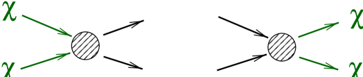
Figure 1: Keeping the $\chi$’s in chemical equilibrium.

At temperatures much larger than the mass of the $\chi$, the number density of $\chi$’s was simply a spin factor times the number density of photons. As the universe expanded and cooled, the temperature eventually fell below the mass of the $\chi$, and the number density of $\chi$’s began to drop exponentially.

$${n_{\chi}\sim\left\{\begin{array}[]{rl}{{\cal O}(1)n_{\gamma}}&{T\gg m_{\chi}}\\[2.15277pt] {n_{\gamma}({m_{\chi}\over T})^{3/2}e^{-m_{\chi}/T}}&{T\mathrel{\raise 1.29167pt\hbox{$<$\kern-7.5pt\lower 4.30554pt\hbox{$\sim$}}}m_{\chi}}\end{array}\right.}$$ (5)

If this were the end of the story, it would be a rather dull tale: since the temperature of the universe today is about $3^{\circ}$ K$\sim 2.5\times 10^{-4}$ eV, the number density of a, say, 100 GeV $\chi$ would be suppressed vis-à-vis that of photons by a factor $\sim\exp\{-4\times 10^{14}\}$. I.e., there would be no $\chi$’s left now. However, in an expanding universe, this conclusion does not hold, because at some point the $\chi$’s fall out of chemical equilibrium with the bath. Specifically, this occurs when the $\chi$ annihilation rate falls below the expansion rate of the universe, $\Gamma_{\rm ann}\mathrel{\raise 1.29167pt\hbox{$<$\kern-7.5pt\lower 4.30554pt\hbox{$\sim$}}}H$. At this point, the $\chi$’s cannot find each other in order to annihilate sufficiently fast for their number density to track the rapid exponential fall of (5). The number density of $\chi$’s subsequently “freezes out” and simply falls with the volume of the universe, $n_{\chi}\sim 1/V$.

Figure 2: The $\chi$’s fall out of chemical equilibrium.

To be more explicit, the number density of $\chi$’s evolves according to the Boltzmann equation,

$${dn_{\chi}\over dt}=-3n_{\chi}H-\langle\sigma_{\rm ann}v\rangle(n_{\chi}^{2}-n_{\chi,{\rm eq.}}^{2})$$ (6)

Here $H=\dot{R}/R$, where $R$ is the scale factor of the universe, and so the first term on the RHS of (6) simply represents the volume suppression of the number density of the $\chi$. The first term in parentheses describes the destruction of the $\chi$ through annihilation, and the last term describes the production of $\chi$ particles from interactions of the thermal bath. An approximate analytic solution to (6) is given by [3]

$$\Omega_{\chi}h^{2}\approx{10^{-10}{\rm GeV}^{-2}\over\sqrt{\,g_{f}}(a+{1\over 2}b)x_{f}},$$ (7)

where $\Omega_{\chi}\equiv\rho_{\chi}/\rho_{c}$ is the present mass density of $\chi$ particles in units of the critical density $\rho_{c}$ required to close the universe, $g_{f}$ is the number of relativistic degrees of freedom at freeze out, $h$ is the current Hubble parameter $H$ in units of 100 km/s/Mpc, and where the thermally averaged annihilation cross-section has been expanded in powers of $(T/m_{\chi})$:

$$\langle\sigma_{\rm ann}v\rangle=a+b\left(T\over m_{\chi}\right)+\ldots$$ (8)

The temperature at freeze-out is typically well below the mass of the $\chi$, so that $x_{f}\equiv T_{f}/m_{\chi}\sim 1/20-1/25$, and eq. (8) is a good expansion. Now, the key feature of (7) is that if the $\chi$ annihilation cross-section is reduced, the $\chi$ freeze out of chemical equilibrium earlier, when their density has had less time to track the exponential Boltzmann suppression (5), and the $\chi$ relic abundance is larger. But a lower bound of 12 Gyr on the age of the universe (along with the assumption that $\Omega_{\rm tot}\leq 1$) implies that $\Omega_{\rm tot}h^{2}\leq 0.3$. Or in other words, a lower bound on the age of the universe implies a lower bound on the $\chi$ annihilation rate, and this is the feature we will primarily exploit to constrain SUSY models.

3.2 Relic Density Constraints

Let us now turn to the MSSM and see what these cosmological considerations do for us. The lightest supersymmetric particle is typically the lightest neutralino, and in many models, including mSUGRA, the lightest neutralino is a quite pure bino $\tilde{B}$. In the early universe, binos annihilate primarily via sfermion exchange into fermion pairs.

Figure 3: Sfermion exchange dominates $\chi$’s annihilation.

Now, if the mass of the sfermions is large, then $\tilde{B}$ annihilation in the early universe is suppressed, and $\Omega_{\widetilde{\chi}}\,h^{2}$ is raised. From the last section, we see that the lower bound on the age of the universe implies an upper bound on the sfermion masses, and hence on both mSUGRA parameters $m_{0}$ and $m_{1\!/2}$. These limits are nicely complementary to those coming from direct searches for SUSY particles, which typically give lower bounds on the SUSY mass parameters.

The cosmological limits can be translated into $\{m_{1\!/2},m_{0}\}$ plane [5], shown in Fig. 4. The light-shaded region corresponds to $0.1\leq\Omega_{\widetilde{\chi}}\,h^{2}\leq 0.3$; the area above this region is excluded. Below this region, $\Omega_{\widetilde{\chi}}\,h^{2}<0.1$, so that another component of the dark matter would be required. This latter is not a bound in the same sense as the upper limit, since we don’t know for certain that any of the dark matter is composed of neutralinos. In the narrow chimney near $m_{1\!/2}=110$GeV, $m_{\tilde{\chi}}\approx m_{h}/2$, and s-channel annihilation through the Higgs pole can bring the relic abundance of neutralinos below 0.3, regardless of the sfermion masses. In the dark shaded region, the LSP is the right-handed stau, which is excluded by the very tight limits on the abundance of charged dark matter [3].

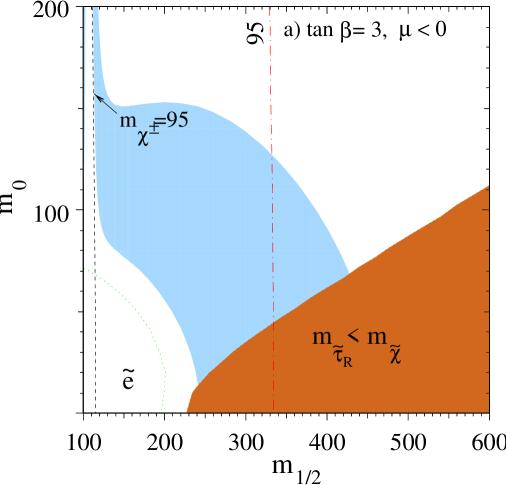
Figure 4: The light-shaded area is the cosmologically preferred region with $0.1\leq\Omega_{\widetilde{\chi}}\,h^{2}\leq 0.3$. In the dark shaded regions in the bottom right of each panel, the LSP is the ${\tilde{\tau}}_{R}$, leading to an unacceptable abundance of charged dark matter. Also shown are the isomass contours $m_{\chi^{\pm}}=95$ GeV and $m_{h}=95$ GeV, as well as an indication of the slepton bound from LEP.

In Fig. 4 we also display current experimental limits: the light dotted contour represents the bound from searches for sleptons at LEP, while the the dashed line is a chargino isomass contour of 95 GeV, which approximates the LEP189 chargino bounds at large $m_{0}$. Note that the chargino bound excludes almost all of the Higgs pole chimney. The most significant experimental bound at this value of $\tan\beta$ comes from Higgs searches at LEP. The dot-dashed contour represents a light Higgs mass of 95 GeV, which approximates the Higgs limit from LEP189, and the bulk of the cosmologically allowed region is excluded. Now, the Higgs mass itself is sensitive to $\tan\beta$, and as $\tan\beta$ is dropped, the dot-dashed contour moves quickly to the right. It is clear that for some value of $\tan\beta$, the Higgs contour moves to the right of the light-shaded region entirely, and this and lower values of $\tan\beta$ are consequently excluded. The current bound at this value of $\tan\beta$ is around 102 GeV [4], and these arguments imply a lower bound on $\tan\beta$ of 3.7 (2.8) for $\mu<0(\mu>0)$. We’ll see in the next section that these constraints are weakened when we consider coannihilation.

4 Coannihilation

4.1 The Basics

So far, we have ignored interactions of the LSP with heavier SUSY particles. Recall that the LSPs freeze out of chemical equilibrium when they’re very cold ($m_{\tilde{\chi}}/T\sim 25$), so that if the mass splitting between the LSP and the next-to-lightest supersymmetric particle (NLSP) is ${\cal O}(1)$, the number density of NLSPs at freeze-out is Boltzmann suppressed with respect to that of LSPs by a factor which is $\sim\exp\{-25\}<10^{-10}$. Therefore we don’t have to worry about NLSP interactions. If, on the other hand, the LSP and NLSP are closely degenerate in mass, then the NLSP interactions near freeze-out may affect the LSP relic density.

This produces two competing effects. First, the NLSPs freeze out of chemical equilibrium with the standard model bath at the same time as the LSPs and subsequently decay into LSPs, and so a significant NLSP abundance at freeze-out can increase the relic LSP density. Typically a larger effect is that since the NLSP interactions contribute to the exchange of particle number between SUSY and standard model particles (and can dominate, as we’ll see below), the SUSY particles remain in chemical equilibrium with the thermal bath for longer and track the equilibrium down to lower temperatures, and this reduces the LSP relic abundance.

How degenerate do the LSP and NLSP states have to be in order to produce a significant effect? Well,

$${\frac{n_{{\scriptscriptstyle\rm NLSP}}}{n_{{\scriptscriptstyle\rm LSP}}}\sim e^{-\Delta m/T}\sim e^{-25(m_{\scriptscriptstyle\rm NLSP}/m_{\scriptscriptstyle\rm LSP}-1)}}.$$ (9)

If the NLSP is 10% (5%) heavier than the LSP, this ratio is $\sim{1\over 10}({1\over 3})$. We see that unless the lightest states are highly degenerate, coannihilation will only be important if $\sigma_{\rm NLSP-LSP}$ (or $\sigma_{\rm NLSP-NLSP}$) $\gg\sigma_{\rm LSP-LSP}$. And mSUGRA (and much of the MSSM), they are!! Consider the temperature expansion of the thermally averaged cross-section (8). When the final state is a fermion pair (the dominant annihilation channel for a $\tilde{B}$-like neutralino), $a\sim m_{f}^{2}$. This dependence is due to the fact that one has identical Majorana fermions in the initial state [6] and is called “p-wave suppression”. Since $T/m_{\tilde{\chi}}$ is small at freeze-out, this suppresses the annihilation rate (and enhances the relic abundance) by an order of magnitude. Coannihilation cross-sections do not have such a suppression and are typically an order of magnitude larger, and the NLSP interactions can therefore dramatically reduce the SUSY relic abundance. These effects have been well studied in SUSY for Higgsino-like neutralinos [7], where there is typically a close degeneracy between the lightest and next-to-lightest neutralinos and the lightest chargino. What we have found is that coannihilation is also an essential element in determining the cosmological upper bound on gaugino ($\tilde{B}$) like neutralinos, as well [8].

4.2 $\tilde{B}-\tilde{\tau}$ Coannihilation

Looking back at Fig. 4, we shouldn’t be surprised that coannihilation may be important in mSUGRA. The upper bound on $m_{1\!/2}$ occurs at the intersection of the $\Omega_{\widetilde{\chi}}\,h^{2}=0.3$ contour with the the top of the region with $m_{\tilde{\tau}_{R}}<m_{\tilde{\chi}}$, i.e. at a point where the stau and neutralino are exactly degenerate! Generally in the MSSM , the cosmological upper bound on the mass of the $\tilde{B}$ is saturated when the masses of the lightest sfermions are degenerate with $m_{\tilde{B}}$. In mSUGRA, the three right-handed sleptons ${\widetilde{\tau}}_{\scriptscriptstyle\rm R},{\widetilde{\mu}}_{\scriptscriptstyle\rm R}$ and ${\widetilde{e}}_{\scriptscriptstyle\rm R}$ are the lightest sfermions and can all be close in mass to the LSP. We must therefore consider [2, 5] the effective annihilation cross-section

$${\sigma_{\rm eff}=\frac{1}{n^{2}}\sum_{ij}\sigma_{ij}n_{i}^{\rm eq}n_{j}^{\rm eq}},$$ (10)

where $i,j={\widetilde{\tau}}_{\scriptscriptstyle\rm R},\;{\widetilde{\tau}}_{\scriptscriptstyle\rm R}^{*},\;{\widetilde{e}}_{\scriptscriptstyle\rm R},\;{\widetilde{e}}_{\scriptscriptstyle\rm R}^{*},{\widetilde{\mu}}_{\scriptscriptstyle\rm R},\;{\widetilde{\mu}}_{\scriptscriptstyle\rm R}^{*}$ and $\widetilde{\chi}$, and where $n=\sum n_{i}$. The complete set of initial and final states contributing to (10) is given in Table LABEL:table:states. The dominant contributions to $\sigma_{\rm eff}$ come from ${\widetilde{\ell}}_{\scriptscriptstyle\rm R}{\widetilde{\ell}}_{\scriptscriptstyle\rm R}^{*}$ annihilation to gauge bosons, ${\widetilde{\ell}}_{\scriptscriptstyle\rm R}{\widetilde{\ell}}_{\scriptscriptstyle\rm R}$ annihilation to lepton pairs and ${\widetilde{\ell}}_{\scriptscriptstyle\rm R}\widetilde{\chi}$ annihilation to a lepton plus a gauge boson. The final states with heavy Higgses turn out to be kinematically unavailable in the regions of interest. For further calculational details, see [8].

Table 2: Initial and Final States for Coannihilation: $\{i,j=\tau,e,\mu\}$

Initial State	Final States
${\widetilde{\ell}}_{\scriptscriptstyle\rm R}^{\,i}\,{\widetilde{\ell}}_{\scriptscriptstyle\rm R}^{\,i^{\scriptstyle*}}$	$\gamma\gamma,\,\,ZZ\,,\,\gamma Z,\,W^{+}W^{-},\,Zh\,,\gamma h\,,\,h\,h,\,f\bar{f},$
	${\rm ZH,\gamma H,ZA,W^{+}H^{-},hH,hA,HH,HA,AA,H^{+}H^{-}}$
${\widetilde{\ell}}_{\scriptscriptstyle\rm R}^{\,i}\,{\widetilde{\ell}}_{\scriptscriptstyle\rm R}^{\,j}$	$\ell^{\,i}\ell^{\,j}$
${\widetilde{\ell}}_{\scriptscriptstyle\rm R}^{\,i}\,{\widetilde{\ell}}_{\scriptscriptstyle\rm R}^{\,{j}^{\scriptstyle*}},\,i\neq j$	$\ell^{\,i}\bar{\ell}^{\,j}$
${\widetilde{\ell}}_{\scriptscriptstyle\rm R}^{\,i}\,\widetilde{\chi}$	$\ell^{\,i}\gamma,\ell^{\,i}Z,\ell^{\,i}h$

In Fig. 5, we show the contributions to $\hat{\sigma}\equiv a+{1\over 2}b\,x_{f}$ (see (7)) for ${\widetilde{\tau}}_{\scriptscriptstyle\rm R}{\widetilde{\tau}}_{\scriptscriptstyle\rm R}^{*}$ annihilation. The top solid contour is the total $\hat{\sigma}$ for ${\widetilde{\tau}}_{\scriptscriptstyle\rm R}{\widetilde{\tau}}_{\scriptscriptstyle\rm R}^{*}$, while for comparison we display as a thick dotted line the equivalent total neutralino annihilation cross-section. As advertised, the stau cross-section is over an order of magnitude greater than that for the neutralinos, which is p-wave suppressed. Figures for ${\widetilde{\tau}}_{\scriptscriptstyle\rm R}-\tilde{\chi}$ and ${\widetilde{\tau}}_{\scriptscriptstyle\rm R}-{\widetilde{\tau}}_{\scriptscriptstyle\rm R}$ annihilation show a similar enhancement over the $\widetilde{\chi}-\widetilde{\chi}$ cross-section, and figures for other $\tan\beta$ and $m_{0}$ are similar.

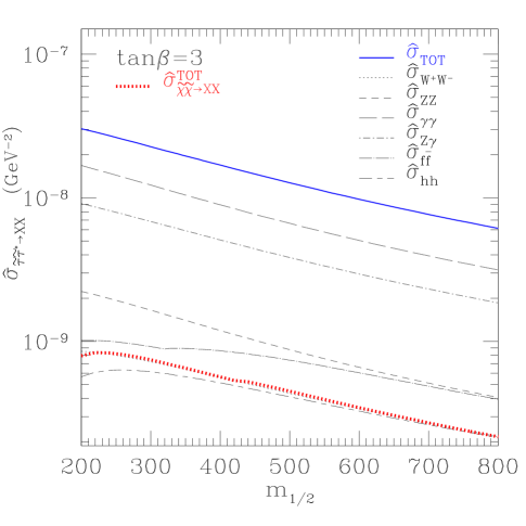
Figure 5: The separate contributions to the ${\widetilde{\tau}}_{\scriptscriptstyle\rm R}{\widetilde{\tau}}_{\scriptscriptstyle\rm R}^{*}$ cross section $\hat{\sigma}\equiv a+{1\over 2}bx$ for $x=T/{m_{\chi}}=1/23$ and $m_{0}=120{\rm\,Ge\kern-1.25ptV}$, as a function of $m_{1\!/2}$. For comparison, the thick dotted line is the $\tilde{\chi}\tilde{\chi}$ cross section.

In Fig. 6, we display the contributions to $\hat{\sigma}_{\rm eff}$ as a function of the fractional mass difference $\Delta M\equiv(m_{\tilde{\tau}_{R}}-m_{\chi})/m_{\chi}$ between the neutralino and the stau. The thick solid contour shows the total $\hat{\sigma}_{\rm eff}$, while for comparison the thin solid contour gives the $\hat{\sigma}_{\rm eff}$ one would compute if one ignored coannihilations, i.e. $a_{\widetilde{\chi}\widetilde{\chi}}+b_{\widetilde{\chi}\widetilde{\chi}}/2$. Here we’ve fixed $m_{1\!/2}=500$ GeV and scanned upwards in $m_{0}$, which increases $\Delta M$. When the neutralino and stau are degenerate, the dominant contribution to $\hat{\sigma}_{\rm eff}$ comes from slepton annihilation. The ratio of the solid contours at this point is greater than an order of magnitude, as above. As $\Delta M$ increases, the density $n_{\tilde{\ell}}^{\rm eq}$ of sleptons becomes Boltzmann suppressed, and the slepton-slepton contribution falls with two powers of $n_{\tilde{\ell}}^{\rm eq}$ and drops below the slepton-neutralino contribution at $\Delta M\sim 0.07$. This contribution in turn falls with one power of $n_{\tilde{\ell}}^{\rm eq}$, and neutralino annihilation becomes dominant again at $\Delta M\sim 0.17$. At large $\Delta M$, the two solid contours and dot-dashed contour merge, and coannihilation can be neglected. Again, figures for other $\tan\beta$ are similar.

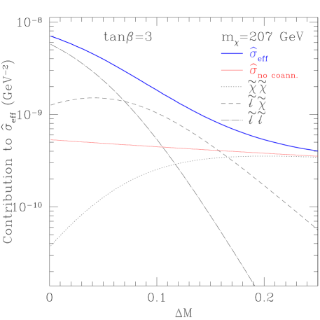
Figure 6: The separate contributions to the cross section $\hat{\sigma}_{\rm eff}$ for $x=T/m_{\chi}=1/23$, as a function of $\Delta M\equiv(m_{\tilde{\tau}_{R}}-m_{\chi})/m_{\chi}$, with $(m_{1\!/2},\tan\beta)=(500$ GeV$,3)$

Let’s now look back at the $\{m_{1\!/2},m_{0}\}$ plane and examine the effect of coannihilation on the cosmologically allowed region. In Fig. 7, we show the same area of parameter space as in Fig. 4, but now with coannihilation included. We see that the light-shaded area now bends away from the forbidden stau LSP region and creates a large allowed trunk which lies on top of the line $m_{\tilde{\tau}_{R}}=m_{\tilde{\chi}}$. Eventually, for large enough $m_{1\!/2}$, the top of the trunk falls below the $m_{\tilde{\tau}_{R}}=m_{\tilde{\chi}}$ line, but this doesn’t happen until much larger values of $m_{1\!/2}$ and $m_{0}$, as seen in Fig. 8. Some features of the new cosmologically allowed region to note: The upper bounds on $m_{0}$ and $m_{1\!/2}$ are relaxed to $m_{1\!/2}\mathrel{\raise 1.29167pt\hbox{$<$\kern-7.5pt\lower 4.30554pt\hbox{$\sim$}}}1400$ GeV and $m_{0}\mathrel{\raise 1.29167pt\hbox{$<$\kern-7.5pt\lower 4.30554pt\hbox{$\sim$}}}350$ GeV, respectively. The width of the new allowed trunk is significant, from 30-50 GeV in $m_{0}$ for $m_{1\!/2}$ up to $\sim 800$ GeV. We’ve only shown the cosmologically interesting region for one value of $\tan\beta$, but the shape is very similar for all small to moderate $\tan\beta$. The position of the line $m_{\tilde{\tau}_{R}}=m_{\tilde{\chi}}$ can vary somewhat with $A_{0}$; however, the width of the trunk above the line is quite insensitive to $A_{0}$, as is the upper bound on $m_{1\!/2}$. This relaxes dramatically the cosmological upper bound on the neutralino mass in mSUGRA from about 200 GeV to close to 600 GeV. It will therefore take the reach of the LHC to probe the full cosmologically interesting region. Lastly, the bounds on $\tan\beta$ from combining the Higgs search limits with relic density constraints are now weakened, from 3.7 (2.8) to 2.8 (2.3) for $\mu<0\;(\mu>0)$.

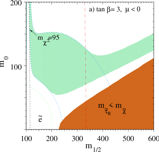
Figure 7: As in Fig. 4, but now including neutralino-slepton coannihilation.

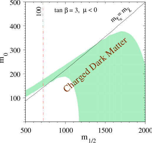
Figure 8: The same as Fig. 7, but extended to larger $m_{1\!/2}$.

5 CP Violation and Electric Dipole Moments

As an application, we’ll now examine to what extent the relaxation of our upper limits on $m_{1\!/2}$ affects constraints on CP violation in the MSSM. We’ll start with a brief reminder of where CP violation arises in our model. Recall that in the MSSM, new CP violating phases $\theta_{\mu}$ and $\theta_{A_{i}}$ accompany the (in principle) complex parameters $\mu$ and $A_{i}$, introduced in the first part of this talk. These phases then appear in the low energy Lagrangian in the neutralino and chargino mass matrices (in the case of $\theta_{\mu}$) and in the left-right sfermion mixing terms (both $\theta_{\mu}$ and $\theta_{A}$). The new sources for CP violation then contribute to the Electric Dipole Moments (EDMs) of standard model fermions, and the tight experimental constraints on the EDMs of the electron, neutron and mercury atom place severe limits on the sizes of $\theta_{\mu}$ and $\theta_{A}$ [12, 13].

The EDMs generated by $\theta_{\mu}$ and $\theta_{A}$ are sufficiently small if either 1) the phases are very small ($\mathrel{\raise 1.29167pt\hbox{$<$\kern-7.5pt\lower 4.30554pt\hbox{$\sim$}}}10^{-2}$), or 2) the SUSY masses are very large (${\cal O}$ (a few TeV)), or 3) There are large cancellations between different contributions to the EDMs. In mSUGRA, option 2) is forbidden by the relic density constraints, as we’ll show next. Condition 3), large cancellations, does naturally occur in mSUGRA models over significant regions of parameter space, including in the body of the cosmologically allowed region with $m_{1\!/2}={\cal O}(100-400\;{\rm GeV})$. These cancellations relax the constraints on the phases, but the limit on $\theta_{\mu}$ remains small, $\theta_{\mu}\mathrel{\raise 1.29167pt\hbox{$<$\kern-7.5pt\lower 4.30554pt\hbox{$\sim$}}}\pi/10$.

To see why option 2) is cosmologically forbidden, recall that the SUSY phases contribute to the electron EDM, for example, via processes of the following type:

where selectrons and sneutrinos appear in the loop. These contributions diminish as the sfermion masses are increased, but this also shuts off neutralino annihilation in the early universe, which is dominated by sfermion exchange as in Fig. 3. The upper bound on $\Omega_{\widetilde{\chi}}\,h^{2}$ then limits the extent to which one can turn off the electron EDMs by raising the sfermion masses. The combination of cosmological with EDM constraints in the MSSM and mSUGRA is discussed in detail in [14, 13].

To see the combined limits on $\theta_{\mu}$ and $\theta_{A}$ in mSUGRA, we plot in the $\{\theta_{\mu},\theta_{A}\}$ plane the minimum value of $m_{1\!/2}$ required to bring the EDMs of both the electron and the mercury atom ¹⁹⁹Hg below their respective experimental constraints (Fig. 9). These experiments currently provide the tightest bounds on the SUSY phases. Here we’ve fixed $\tan\beta=2$, $A_{0}=300$ GeV and $m_{0}=100$ and scanned upwards in $m_{1\!/2}$ until the experimental constraints are satisfied. Due to cancellations, the EDMs are not monotonic in $m_{1\!/2}$; however, there is still a minimum value of $m_{1\!/2}$ which is allowed. Looking back at Fig. 4, we see that in the absence of coannihilations, there is an upper bound on $m_{1\!/2}$ of about 450 GeV (though slightly smaller for this $m_{0}$); an analogous figure to Fig. 7 for $\tan\beta=2$ shows that coannihilations increase the bound to about 600 GeV. Comparing with Fig. 9, we see that zone V is cosmologically forbidden, and that the effect of including coannihilations is to allow zone IV, which was formerly excluded.

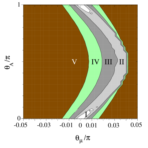
Figure 9: Contours of $m_{1\!/2}^{\rm min}$, the minimum $m_{1\!/2}$ required to bring both the electron and Hg EDMs below their respective experimental bounds, for $\tan\beta=2,m_{0}=130{\rm\,Ge\kern-1.25ptV}$, and $A_{0}=300{\rm\,Ge\kern-1.25ptV}$. The central light zone labeled “I” has $m_{1\!/2}^{\rm min}<200{\rm\,Ge\kern-1.25ptV}$, while the zones labeled “II”, “III”, and “IV” correspond to $200{\rm\,Ge\kern-1.25ptV}<m_{1\!/2}^{\rm min}<300{\rm\,Ge\kern-1.25ptV}$, $300{\rm\,Ge\kern-1.25ptV}<m_{1\!/2}^{\rm min}<450{\rm\,Ge\kern-1.25ptV}$, $450{\rm\,Ge\kern-1.25ptV}<m_{1\!/2}^{\rm min}<600{\rm\,Ge\kern-1.25ptV}$ and $m_{1\!/2}^{\rm min}>600{\rm\,Ge\kern-1.25ptV}$, respectively. Zone V is therefore cosmologically excluded.

Note in particular that the overall upper bound on $\theta_{\mu}$ in this figure, $\theta_{\mu}\mathrel{\raise 1.29167pt\hbox{$<$\kern-7.5pt\lower 4.30554pt\hbox{$\sim$}}}0.04\pi$, is not affected by coannihilations. This is because the largest $\theta_{\mu}$ occur in regions of cancellations, and these regions happen to lie at lower values of $m_{1\!/2}$, starting in zone II with $m_{1\!/2}<300$ GeV. Increasing $m_{1/2}^{\rm max}$ from 450 to 600 GeV is insufficient to bring the individual contributions to the EDMs to acceptable levels for the larger values of $\theta_{\mu}$ and significant cancellations are still necessary. Even taking $m_{1\!/2}$ and $m_{0}$ at their maximal values from Fig. 7 is not sufficient to reduce the EDMs below their experimental limits, and so coannihilation does not affect the upper bound on $\theta_{\mu}$.

The bowing to the right of the contours in Fig. 9 is a result of cancellations between different contributions to the EDMs [14], and we can see that the effect is to relax the upper bound on $\theta_{\mu}$ by a factor of a few. As we increase $A_{0}$, the extent of the bowing increases, and larger values of $\theta_{\mu}$ can be accessed. This loophole to larger $\theta_{\mu}$ is limited by the diminishing size of the regions in which there are sufficient cancellations to satisfy the EDM constraints. In general, the regions of cancellation for the electron EDM are different than those for the ¹⁹⁹Hg EDM, and the two regions do not always overlap. As $\theta_{\mu}$ is increased, the sizes of the regions of sufficient cancellations decrease; in Fig. 9, the width in $m_{1\!/2}$ of the combined allowed region near the $\theta_{\mu}$ upper bound is 40-80 GeV, which on a scale of 200-300 GeV is reasonably broad. Larger $A_{0}$ permits larger $\theta_{\mu}$, but the region of cancellations shrinks so that a careful adjustment of $m_{1\!/2}$ becomes required to access the largest $\theta_{\mu}$. At the end of the day, values of $\theta_{\mu}$ much greater than about $\pi/10$ cannot satisfy the EDM constraints without significant fine-tuning of the mass parameters. At larger values of $\tan\beta$, the upper bound decreases roughly as $1/\tan\beta$. See [13] for more details on the status of EDM and cosmological constraints on CP violating phases in mSUGRA.

6 Summary

In summary, constraints on the relic abundance of LSP neutralinos place significant restrictions on the parameter space of the MSSM, and mSUGRA in particular. To accurately compute the cosmological upper limits on MSSM masses requires the inclusion of coannihilation effects, both for the case of a Higgsino and gaugino like neutralino. In particular, we have found that slepton-neutralino coannihilation greatly affects the neutralino relic abundance when the neutralino and slepton are closely degenerate in mass, as is the case in mSUGRA near where the cosmological upper bound on the neutralino mass is saturated. Including coannihilation effects significantly relaxes the cosmological bounds on $m_{1\!/2},m_{0}$ and $m_{\tilde{\chi}}$, and reduces the combined Higgs + cosmology lower bound on $\tan\beta$, although the upper bounds on CP violating phases in mSUGRA are not relaxed. The reach of the LHC will be needed to be sensitive the full cosmologically allowed region. Lastly, although I did not discuss it here, similar effects are present for a gaugino like neutralino in the general MSSM.

Acknowledgments
The work of T.F. was supported in part by DOE grant DE–FG02–95ER–40896 and in part by the University of Wisconsin Research Committee with funds granted by the Wisconsin Alumni Research Foundation.

References

- [1] S. Dimopoulos and D. Sutter, Nucl. Phys. B452 (1995) 496.
- [2] K. Griest and D. Seckel, Phys. Rev D43 (1991) 3191; P. Gondolo and G. Gelmini, Nucl. Phys. B360 (1991) 145.
- [3] J. Ellis, J.S. Hagelin, D.V. Nanopoulos, K.A. Olive and M. Srednicki, Nucl. Phys. B238 (1984) 453.
- [4] ALEPH, DELPHI, L3 and OPAL Collaborations, ALEPH-99-081, DELPHI 99-142, L3 Note 2442, OPAL Technical Note TN-614 (submitted to the International Europhysics Conference on High Energy Physics, Tampere, Finland).
- [5] J. Ellis, T. Falk, K.A. Olive and M. Schmitt, Phys. Lett. B388 (1996) 97; J. Ellis, T. Falk, K.A. Olive and M. Schmitt, Phys. Lett. B413 (1997) 355.
- [6] H. Goldberg, Phys. Rev. Lett. 50 (1983) 1419.
- [7] M. Drees, M.M. Nojiri, D.P. Roy and Y. Yamada, Phys. Rev. D56 (1997) 276.
- [8] J. Ellis, T. Falk, and K.A. Olive, Phys. Lett. B444 (1998) 367; J. Ellis, T. Falk, K.A. Olive and M. Srednicki, hep-ph/9905481.
- [9] K.F. Smith et al., Phys. Lett. B234 (1990) 191; I.S. Altarev et al., Phys. Lett. B276 (1992) 242.
- [10] J.P. Jacobs et al., Phys. Rev. Lett. 71 (1993) 3782; J.P. Jacobs et al., Phys. Rev. A52 (1995) 3521.
- [11] E.D. Commins et al., Phys. Rev. A50 (1994) 2960.
- [12] M. Dugan, B. Grinstein and L. Hall, Nucl. Phys. B255, 413 (1985); Y. Kizukuri & N. Oshimo, Phys. Rev. D45 (1992) 1806; D46(1992) 3025.
- [13] T. Falk, K.A. Olive, M. Pospelov and R. Roiban, hep-ph/9904393.
- [14] T. Falk, K.A. Olive and M. Srednicki, Phys.Lett. B354 (1995) 99; T. Falk and K. Olive, Phys. Lett. B375 (1996) 196; T. Falk and K.A. Olive, Phys. Lett. B439 (1998) 71.