CP Violaing Phases In SUSY GUT Models

Abstract

Supersymmetric CP violating phases are examined within the framework of gravity mediated supergravity grand unified models with R parity invariance for models with a light ($\stackrel{{\scriptstyle<}}{{\sim}}1$ TeV) particle spectrum. In the minimal model, the nearness of the t quark Landau pole naturally suppresses the t-quark cubic soft breaking parameter at the electroweak scale allowing the electron and neutron experimental electric dipole moment (EDM) constraints to be satisfied with a large GUT scale phase. However, the EDM constraints require that $\theta_{B}$, the quadratic soft breaking parameter phase be small at the electroweak scale unless tan$\beta\stackrel{{\scriptstyle<}}{{\sim}}3$, which then implies that at the GUT scale this phase must be large and highly fine tuned to satisfy radiative breaking of $SU(2)\times U(1)$. Similar results hold for non minimal models, and a possible GUT model is discussed where all GUT scale CP violating phases are naturally small (i.e. O($10^{-2})$). An interesting D-brane model is examined which enhances the size of the phases over much of the parameter space at the electroweak sector for tan$\beta\stackrel{{\scriptstyle<}}{{\sim}}5$, but still possesses the fine tuning problem at the GUT scale.

1 Introduction

The Standard Model (SM) of strong and electroweak interactions is a remarkably rigid theory of quark and lepton interactions. Thus the gauge invariance guarantees baryon and lepton number invariance and forbids bare mass terms. In order to generate quark and lepton masses, one introduces Higgs Yukawa couplings, and the spontaneous breaking of $SU(2)\times U(1)$ simultaneously generates the necessary masses, both in the gauge boson and fermionic sectors. For the three generations that have been observed, the Yukawa matrices allow for only one CP violating phase in the CKM matrix, which is consistent with the observed CP violation in the K meson system (and these ideas will be tested for B mesons with future data from B factories and high energy accelerators.). Further this phase gives only a very small contribution to the electron and neutron electric dipole moments (EDMs), $d_{e}$ and $d_{n}$. In supersymmetry (SUSY) extensions of the SM, things are more complicated. One generally imposes R-parity invariance to suppress too rapid proton decay, and there is now an array of possible new CP violating phases arising from the SUSY soft breaking masses which generally produce large contributions to $d_{n}$ and $d_{e}$. The current experimental EDM bounds are for $d_{n}$[1] and $d_{e}$ [2]:

$$(d_{n})_{exp} < 6.3\times 10^{-26}ecm;\,90\%C.L.$$ (1)

$$(d_{e})_{exp} < 4.3\times 10^{-27}ecm;\,95\%C.L.$$ (2)

In the past, two suggestions have been made to accomodate these bounds: (i) one can assume the CP violating phases are small i.e. $\phi=O(10^{-2})$[3] and/or (ii) the SUSY mass spectrum is heavy i.e. squark ($\tilde{q}$), slepton ($\tilde{l}$) and gluino ($\tilde{g}$) masses are $\stackrel{{\scriptstyle>}}{{\sim}}O(1{\rm TeV})$ [4]. The first hypothesis would appear to require a significant amount of fine tuning(though see sec. 4 below), while the second would place the SUSY spectrum beyond the reach of even the LHC and regenerate the gauge hierarchy problem. Recently, it has been observed that a third option is possible, i.e. that cancellations can naturally occur in the total EDM amplitude (e.g. between neutralino and chargino contributions) allowing one to satisfy Eqs. (1,2) with relatively large phases (i.e. O($10^{-1}$)) and a light SUSY spectrum $<O(1{\rm TeV})$ [5]., and there has been considerable investigation of this possibility [5, 6, 7, 8, 9, 10, 11, 13, 14]. The work presented here is given in Ref[15, 16].

We consider here these possibilities within the framework of supergravity (SUGRA) grand unified models (GUTs) with gravity mediated SUSY breaking and R-parity invariance [17]. For other work within this framework see [5, 6, 8, 9, 12, 13]. Here the low energy predictions of the model are determined from the GUT scale $M_{G}$ parameters by running the renormalization group equation from $M_{G}$ to the electroweak scale $M_{\rm EW}$. Such a theory is considerably more constrained than the purely phenomenological low energy MSSM model. Thus (1) there are considerable constraints arising from the GUT group symmetry, (2) CP violating phases and SUSY parameters that are arbitrary in the MSSM get correlated by the RGE, (3) radiative breaking of $SU(2)\times U(1)$ at M_EW puts additional constraints on the CP violating phases and SUSY parameters.

In models of this type, what is natural or unnatural is a property of the theory at $M_{G}$ rather than $M_{\rm EW}$. Thus we find that some phases that are naturally large at $M_{G}$ get suppressed at $M_{\rm EW}$ leading, hence, to a “naturally” small phase there. However, unless tan$\beta\stackrel{{\scriptstyle<}}{{\sim}}$3 (assuming SUSY masses are not large) one phase at $M_{\rm EW}$ is quite small, and the RGE then implies that it is both large and highly fine tuned at $M_{G}$. In addition, while there is considerable theretical uncertainty in the calculation of $d_{n}$, the combined constraints of $d_{n}$ and $d_{e}$ of Eqs. (1,2) put significant additional constraints on the allowed SUSY parameter space.

The above results hold for both for the minimal mSUGRA model and generally for models with nonuniversal soft breaking. We will also discuss one very intersting D-brane model with nonuniversal soft breaking [12].

2 Electric Dipole Moments For mSUGRA Models

We consider first the simplest case where there is universal SUSY soft breaking parameters at $M_{G}$. The theory then depends on five parameters: $m_{0}$ (the universal squark and slepton mass at $M_{G}$), $m_{1/2}$ (the universal gaugino mass at $M_{G}$), $A_{0}$ (the cubic soft breaking parameter at $M_{G}$), B₀(the quadratic soft breaking parameter at $M_{G}$) and $\mu_{0}$ (the Higgs mixing parameter at $M_{G}$ in the superpotential). Of these the last four can be complex. However, one may make a phase rotation to make $m_{1/2}$ real, leaving $A_{0}$, $B_{0}$ and $\mu_{0}$ complex at $M_{G}$:

$$A_{0} = |A_{0}|e^{i\alpha_{0A}};\,B_{0}=|B_{0}|e^{i\theta_{0B}};\,\mu_{0}=|\mu_{0}|e^{i\theta_{0\mu}}.$$ (3)

The RGE determines the low energy parameters in terms of the $M_{G}$ parameters. Thus there results a different A parameter at $M_{\rm EW}$ (which we take to be $m_{t}$), for each squark and slepton e.g. $A_{t}$, $A_{b}$,$A_{\tau}$,$A_{u}$, $A_{d}$, $A_{e}$ and we label these by

$$A_{t} = |A_{t}|e^{i\alpha_{t}};\,B=|B|e^{i\theta_{B}};\,\mu=|\mu|e^{i\theta_{\mu}};etc$$ (4)

(Note that to one loop order $\theta_{0\mu}=\theta_{\mu}$.) The $SU(3)_{C}$, $SU(2)_{L}$ and $U(1)_{Y}$ gaugino masses are labeled $\tilde{m}_{3}$, $\tilde{m}_{2}$ and $\tilde{m}_{1}$ and remain real at one loop..

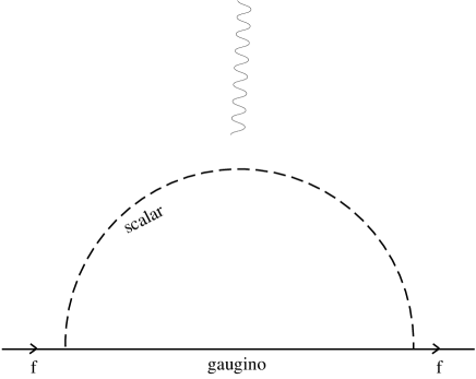
The effective Lagrangian for $d_{f}$, the EDM of fermion of type f (quark or lepton) is

$$L_{f} = -{i\over 2}d_{f}\bar{f}\sigma_{\mu\nu}\gamma^{5}fF^{\mu\nu}.$$ (5)

The basic diagrams for $d_{f}$ that contribute to $L_{f}$ at $M_{\rm EW}$ are given in Fig.1.

The calculation of the neutron EDM contains a number of uncertainties due to QCD effects. To relate $d_{n}$ to the quark EDMs $d_{u}$ and $d_{d}$, we use the non relativistic quark model relation

$$d_{n} = {1\over 3}(4d_{d}-d_{u})$$ (6)

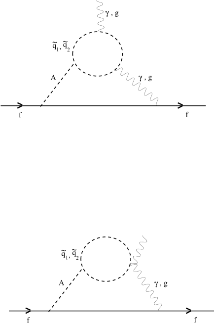
. In addition to Eq.5, one must take into account the gluonic operators $L^{C}$ and $L^{G}$ given by

$$L^{C} = -{i\over 2}d^{C}\bar{q}\sigma_{\mu\nu}\gamma^{5}T^{a}qG_{a}^{\mu\nu}$$ (7)

$$L^{G} = -{1\over 3}d^{G}f_{abc}G_{a\mu\alpha}G_{b\nu}^{\alpha}\tilde{G}_{c}^{\mu\nu}$$ (8)

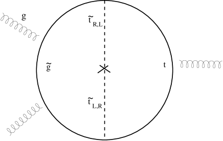
where $\tilde{G}^{\mu\nu}_{c}={1\over 2}\epsilon^{\mu\nu\alpha\beta}G_{c\alpha\beta}$ $(\epsilon^{0123}=1)$, $T^{a}={1\over 2}\lambda^{a}$( $\lambda^{a}$ are the SU(3) Gell-Mann matrices), ${G}^{\mu\nu}_{a}$ are the SU(3) field strengths and $f_{abc}$ are the SU(3) structure constants. Contributions to $L^{C}$ arise from Fig.1 with $\gamma$ replaced by $g$ and the two loop Barr-Zee type diagrams of Fig.2[18]. Contributions to $L^{G}$ come from the two loop Weinberg type diagram of Fig.3 [19]. One must use the QCD RGE factors $\eta^{ED}$, $\eta^{G}$, $\eta^{C}$ to evolve the results from $M_{\rm EW}$ down to 1 GeV [20] and we use the naive dimensional analysis[21] to relate $d^{C}$ and $d^{G}$ to $d_{f}$. In calculating $d_{q}$, one needs to know the quark masses $m_{u}$ and $m_{d}$. While the mass ratios are fairly well known [22],

$${m_{u}\over m_{d}} = 0.553\pm 0.043;\,\,\,\,{m_{s}\over m_{d}}=18.9\pm 0.8$$ (9)

$m_{s}$ is in considerable doubt, i.e. QCD sum rules give $m_{s}=(175\pm 25)$ MeV and lattice gauge theory gives $m_{s}(2GeV)=(100\pm 20\pm 10)$ MeV in the quenched lattice calculation. (Lowering the scale to 1 GeV will increase $m_{s}$, but unquenching will reduce it).

We see in general that there are significant uncertainties in calculating $d_{n}$ ( perhaps a factor of 2-3). In the following we will assume $m_{s}=150$ GeV ($m_{d}\cong$ 8 MeV, $m_{u}\cong$ 4.4 MeV), but we will exhibit below the sensitivity of $d_{n}$ to the uncertainty in $m_{s}$.

$SU(2)\times U(1)$ breaking at $M_{\rm EW}$ gives rise to Higgs VEVs which in general may be complex:

$$<H_{1,2}>=v_{1,2}e^{i\epsilon_{1,2}};\,v_{1,2}\equiv|<H_{1,2}>|$$ (10)

and we define $tan\beta=v_{2}/v_{1}$. One may chose matter phases so that the chargino mass matrix takes the form:

$$M_{\chi^{\pm}} = \left(\matrix{\tilde{m}_{2}&\sqrt{2}M_{W}sin\beta\cr\sqrt{2}M_{W}cos\beta&-|\mu|e^{i\theta}}\right)$$ (11)

where $\theta=\epsilon_{1}+\epsilon_{2}+\theta_{\mu}$. The neutralino mass matrix is:

$$M_{\chi^{0}} = \left(\matrix{\tilde{m}_{1}&0&a&b\cr 0&\tilde{m}_{2}&c&d\cr a&c&0&|\mu|e^{i\theta}\cr b&d&|\mu|e^{i\theta}&0\cr}\right)$$ (12)

where $a=-M_{Z}sin\theta_{W}cos\beta$, $b=M_{Z}sin\theta_{W}sin\beta$, $c=-cot\theta_{W}a$, $d=-cot\theta_{W}b$. The squark mass matrices is

$$M_{\tilde{q}}^{2} = \left(\matrix{m^{2}_{q_{L}}&e^{-i\alpha_{q}}m_{q}(|A_{q}|+|\mu|R_{q}e^{i(\theta+\alpha_{q})})\cr e^{i\alpha_{q}}m_{q}(|A_{q}|+|\mu|R_{q}e^{-i(\theta+\alpha_{q})})&m^{2}_{q_{R}}}\right)$$ (13)

where $m_{q}$, $e_{q}$ are the quark mass and charge,

$$m_{q_{L}}^{2} = m^{2}_{Q}+m_{q}^{2}+(1/2-e_{q}sin^{2}\theta_{W})M_{Z}^{2}cos2\beta$$ (14)

$$m_{q_{R}}^{2} = m^{2}_{U}+m_{q}^{2}+e_{q}sin^{2}\theta_{W}M_{Z}^{2}cos2\beta$$ (15)

where $R_{q}=cot\beta(tan\beta)$ for u(d) quarks and $m_{Q}^{2}$, $m_{U}^{2}$ are given in [23]. (A Similar result holds for the sleptons).

The Higgs VEVs are determined by minimizing the effective potential

$$V_{eff} = m_{1}^{2}v_{1}^{2}+m_{2}^{2}v_{2}^{2}+2|B\mu|cos(\theta+\theta_{B})v_{1}v_{2}+{g^{2}_{2}\over 8}(v_{1}^{2}-v_{2}^{2})^{2}$$

$$+ {{g^{\prime}}^{2}\over 8}(v_{2}^{2}-v_{1}^{2})^{2}+V_{1}$$

where $V_{1}$ is the one loop contribution

$$V_{1}={1\over{64\pi^{2}}}\sum_{a}C_{a}(-1)^{2j_{a}}(2j_{a}+1)m_{a}^{4}(ln{m_{a}^{2}\over Q^{2}}-{3\over 2}).$$ (17)

Here $C_{a}$, $j_{a}$ and $m_{a}$ are the color factor, spin and mass of particle $a$ and $Q=m_{t}$ is the electroweak scale. In the following we include the full third generation of states in $V_{1}$ (t, b $\tau$) so that we can consider large tan$\beta$. The minimization of the tree contribution gives

$$\theta=\pi-\theta_{B}.$$ (18)

From Eq.(13), the mass eigenvalues entering into Eq.(17) depends only on $\theta+\alpha_{q}$ and $\theta+\alpha_{l}$, so that minimizing the tree plus loop $V_{\rm eff}$ gives

$$\theta=\pi-\theta_{B}+f_{1}(\pi-\theta_{B}+\alpha_{q},\pi-\theta_{B}+\alpha_{l})$$ (19)

where $f_{1}$ is the one loop correction. As we will see, this correction can become significant for large tan$\beta$. However, as we will see below, it can make important contributions for large tan$\beta$ since the EDMs are sensitive to $\theta_{B}$.

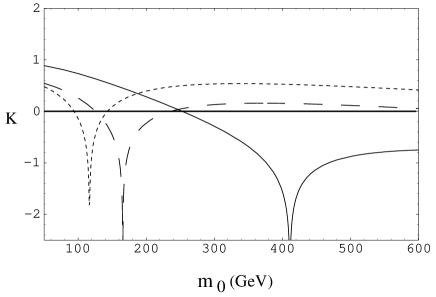
A convenient way of characterizing how close the theory is in accord with the EDMs is given by the parameter K:

$$K=log_{10}\mid{d_{f}\over{(d_{f})_{exp}}}\mid$$ (20)

where $(d_{f})_{exp}$ is the current experimental bound. Thus $K\leq 0$ is required for the theory to be in accord with experiment. An example of K as a function of $m_{0}$ is given in Fig.4. One sees that the width of the allowed $K\leq 0$ region decreases as tan$\beta$ increases. Eventually, for very large $m_{0}$, one would obtain $K<0$ even for large tan$\beta$ (the heavy SUSY spectrum option). For $m_{0}<1$ TeV, we see that the region $K\leq 0$ moves to ower $m_{0}$. The reason for this is that the chargino diagram increases more rapidly with tan$\beta$ than the neutralino diagram, and in order to maintain the cancelation between them to satisfy $K\leq 0$ one must decrease $m_{0}$ to enhance the neutralino diagram relative to the chargino. The above discussion shows that the cancelations needed to achieve $K\leq 0$ are relatively delicate, and would become increasingly so if e.g. the experimental bounds are reduced by a factor of 10 ($K\leq-1$).

To understand what parameters control cancelations, one may look at the RGE which relate the GUT scale parameters to electroweak scale parameters. The one loop RGE must be solved numerically. However, for small or intermediate tan$\beta$ (and also in the SO(10) limit) analytic solutions are availbale which allow one to see analytically what is happenning. Thus for low tan$\beta$ one finds for $A_{t}$ the result

$$A_{t} = D_{0}A_{0}+\Phi_{A}m_{1/2}$$ (21)

where $\Phi_{A}$ is real and O(1) and $D_{0}\cong 1-(m_{t}/{200sin\beta})^{2}$. Thus $D_{0}$ is small i.e. $D_{0}\stackrel{{\scriptstyle<}}{{\sim}}0.2$ . The imaginary part of Eq.(21) gives:

$$|A_{t}|sin\alpha_{t} = |A_{0}|D_{0}sin\alpha_{0A}$$ (22)

Thus because $D_{0}$ is small (the nearness of the t-quark Landau pole) the phase $\alpha_{t}$ is suppressed relative to $\alpha_{0A}$. Thus even if $\alpha_{0A}=\pi/2$, $\alpha_{t}$ is sufficiently reduced at the electroweak scale so that the EDM constraints may be satisfied. Hence in mSUGRA, no fine tuning of $\alpha_{0A}$ is necessary.

The situation, however, is more difficult for the $\theta_{B}$ phase. For low and intermediate tan$\beta$ (and similar results hold for large tan$\beta$ in the SO(10) limit) the RGE solution is

$$B = B_{0}-{1\over 2}(1-D_{0})A_{0}+\Phi_{B}m_{1/2}$$ (23)

where $\Phi_{B}$=real and $O(1)$. The imaginary and real parts give

$$|B|sin\theta_{B} = |B_{0}|sin\theta_{0B}-{1\over 2}(1-D_{0})|A_{0}|sin\alpha_{0A}$$ (24)

$$|B|cos\theta_{B} = |B_{0}|cos\theta_{0B}-{1\over 2}(1-D_{0})|A_{0}|cos\alpha_{0A}+\Phi_{B}m_{1/2}.$$ (25)

These may be viewed as equations to determine $|B|$ and $\theta_{B}$ in terms of the GUT scale parameters. Alternatively, one may impose phenomenological constraints at the electroweak scale to see what GUT scale parameters will satisfy them. Two such constraints are the experimental EDM bounds, and the requirement of radiative breaking of $SU(2)\times U(1)$ at the electroweak scale. The latter implies that

$$|B| = {1\over 2}sin{2\beta}{m_{3}^{2}\over|\mu|}$$ (26)

where $m_{3}^{2}=2|\mu|^{2}+m_{H_{1}}^{2}+m_{H_{2}}^{2}+1{\rm loop}$, where $m_{H_{i}}^{2}$ are the Higgs running masses.

The EDM constraints, generally require that $\theta_{B}$ be small i.e. $\theta_{B}\stackrel{{\scriptstyle<}}{{\sim}}0.2$. Since ${1\over 2}sin2\beta\simeq(1/tan\beta)$, the r.h.s. of Eq.(26) is a decreasing function of tan$\beta$, and hence it determines $|B|$ to be small unless $tan\beta\stackrel{{\scriptstyle<}}{{\sim}}$3. Returning to Eq.(24), one sees that the l.h.s. is thus quite small and so $\theta_{0B}$ is scaled by $\alpha_{0A}$. Hence if $\alpha_{0A}$ is not fine tuned to be small, we find that the GUT scale $\theta_{0B}$ must be large i.e. $O(1)$. (This is indeed confirmed by detailed numerical calculations.) Consider now the situation where one fixes $A_{0}$ at $M_{G}$, and let $\Delta\theta_{B}$ be the allowed range of $\theta_{B}$ satisfying the EDM constraints. One has $\Delta\theta_{B}\stackrel{{\scriptstyle<}}{{\sim}}0.2$ and in general smaller. From Eq. (24) we see the corresponding allowed range at $M_{G}$ is

$$\Delta\theta_{0B}\cong{|B|\over{|B_{0}|}}\Delta\theta_{B}\ll\Delta\theta_{B}$$ (27)

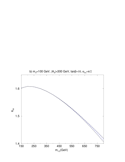
and by $SU(2)\times U(1)$ breaking constraint Eq. (26) one will have $\Delta\theta_{0B}<<\Delta\theta_{B}$ unless tan$\beta\stackrel{{\scriptstyle<}}{{\sim}}$3. Fig.5, where the value of $\theta_{0B}$ obeying the EDM constraint is plotted as a function of $m_{1/2}$ for $|A_{0}|=300$ GeV and $\alpha_{0A}=\pi/2$ illustrates this effect. One sees that indeed $\theta_{0B}$ is large, and that even for tan$\beta$=3, the allowed range of $\Delta\theta_{0B}$ satisfying the $d_{e}$ constraint for $m_{1/2}\stackrel{{\scriptstyle<}}{{\sim}}$350 GeV ($m_{\tilde{g}}\stackrel{{\scriptstyle<}}{{\sim}}$1 TeV) is quite small. For tan$\beta$=10, $\Delta\theta_{0B}$ is very small. (Note that the LEP bound on the Higgs mass already requires tan$\beta\geq$2.)

We see that the combined requirements of radiative electroweak breaking and the experimental EDM constraints lead to a serious fine tuning problem at the GUT scale: $\theta_{0B}$ is large and must be tightly fine tuned unless tan$\beta$ is close to its minimum value tan$\beta$=2 (unless SUSY masses are large, e.g. $\stackrel{{\scriptstyle>}}{{\sim}}$ 1 TeV, and/ or all phases are small, e.g. $O(10^{-2})$. )

We discussed above the existence of uncertainties in calculating of the neutron EDM. We exhibit here the effect of the uncertainty in $m_{s}$ in Eq.(9). Fig.6 plots $K=0$ contours corresponding to $m_{d}$(1 GeV)=5,8 and 12 MeV for tan$\beta$=3, $|A_{0}|=300$ GeV and $\alpha_{0A}=\pi/2$. These values of $m_{d}$ correspond to $m_{s}\cong$ 95, 151 and 227 MeV respectively. (Current lattice calculations favor the lowest value.) We see that $d_{n}$ is quite sensitive to $m_{d}$, the constraint being significantly less severe for the lower quark masses. In Fig.5 and subsequent figures, we have chosen the central value of $m_{d}$= 8 MeV.

We also have mentioned above that the loop corrections in Eq. (19) can be significant for large tan$\beta$. This is because $f_{1}$ which grows with tan$\beta$, represents an effective shift in $\theta_{B}$, and the EDM constraints require $\theta_{B}$ to be small. One can see this effect of $f_{1}$ in Fig. 7 for tan$\beta$=20, where we have set $\theta_{B}=0$ so that in this example $f_{1}$ is the total “effective” $\theta_{B}$ in Eq. (19). For large $m_{1/2}$, the shape of the curves resemble those of Fig.6. However for 175 GeV$\stackrel{{\scriptstyle<}}{{\sim}}m_{1/2}\stackrel{{\scriptstyle<}}{{\sim}}400$ GeV, the $f_{1}$ contribution gives rise to cancelation in the EDM amplitudes to significantly reduce the excluded regions showing that the loop contributions are important for large tan$\beta$. Note that the effect persists even for $K=-0.5$.

3 D-Brane Models

In SUGRA models, nonuniversal soft breaking can arise if the hidden sector fields in the Kahler potential which give rise to SUSY breaking do not couple universally to the physical sector fields. In this case nonuniversal squark, slepton and Higgs masses can be generated at $M_{G}$, as well as nonuniversal A parameters. For simple GUT groups, however, it is difficult to generate more than small nonuniversalties in the gaugino masses at $M_{G}$. Models of this type behave qualitatively similar to the mSUGRA model discussed in Sec.II above i.e. no serious fine tuning is needed for $\alpha_{0A}$, but $\theta_{0B}$ is generally large and highly fine tuned unless tan$\beta\stackrel{{\scriptstyle<}}{{\sim}}$3.

We consider in this section a class of models based on Type IIB orientifolds where the existence of open string sectors imply the presence of $Dp$-branes, manifolds of p+1 dimensions in the full D=10 space of which 6 dimensions are compactified e.g. on a six torus $T^{6}$. (For a general discussion of this class of models see [24]). Models of this type can contain 9 branes (the full 10 dimensional space) plus $5_{i}$-branes, i=1, 2, 3 (6 dimensional space with two compact dimensions) or in the T-dual representation, 3 branes plus 7_i branes, i=1, 2, 3 . Associated with a set of n coincident branes is a gauge group U(n).

One can clearly embed the Standard model gauge group in a number of ways in such models. Recently, an interesting model has been proposed based on 9-branes and 5-branes [12]. In this model, $SU(3)_{C}\times U(1)_{Y}$ is associated with one set of 5-branes, i.e. $5_{1}$, and SU(2)_L is associated with a second intersecting set 5₂. Strings starting on 5₂ and ending on 5₁ have massless modes carrying the joint quantum numbers of the two branes i.e. the SM quark, lepton and Higgs doublets. Strings beginning and ending on 5₁ have massless modes carrying $SU(3)_{C}\times U(1)_{Y}$ quantum numbers i.e. the SM quark and lepton singlets. We assume all other possible fields at the compactification scale $M_{c}$ are superheavy and can be ignored to first approximation, as far as the low energy predictions of the model are concerned. For models of this type $M_{c}=M_{G}$, while the string scale $M_{\rm str}$, is given by $M_{\rm str}=(\alpha_{G}M_{c}M_{Planck}/\sqrt{2})^{1/2}\cong 8\times 10^{16}$ GeV (for $\alpha_{G}\cong 1/24$). Thus below $M_{G}$, the gauge interactions are the ususal D=4 theory.

The gauge kinetic functions for 9 branes and 5_i-branes are given by [24, 25] $f_{9}=S$ and $f_{5_{i}}=T_{i}$ where S is the dilaton and $T_{i}$ are moduli. The origin of SUSY breaking is not yet understood in string theory. It may be parametrized, however, by VEV growth of $S$ and $T_{i}$. Further, in string theory, CP violation must also occur as a spontaneous breaking and it is natural to associate thses two spontaneous breakings by assuming that the F-components grow complex VEVs which are parametrized by [24, 26, 27]

$$F^{S} = {2\sqrt{3}}<{\rm Re}S>{\rm sin}\theta_{b}e^{i\alpha_{s}}m_{3/2}$$ (28)

$$F^{T_{i}} = {2\sqrt{3}}<{\rm Re}T_{i}>{\rm cos}\theta_{b}\Theta_{i}e^{i\alpha_{i}}m_{3/2}$$

where $\theta_{b}$, $\Theta_{i}$ are Goldstino angles ($\sum\Theta_{i}^{2}=1$) and $m_{3/2}$ is the gravitino mass. In the following we assume $\Theta_{3}=0$, $<ReT_{i}>$ are equal (to guarantee grand unification at $M_{G}$), and $<ImT_{i}>$=0 (so that the spontaneous breaking does not grow a $\theta$-QCD type term).

The above model then leads to the following soft breaking masses at $M_{G}$:

$$\tilde{m_{1}} = \sqrt{3}{\rm cos}\theta_{b}\Theta_{1}e^{-i\alpha_{1}}m_{3/2}=\tilde{m_{3}}=-A_{0}$$ (29)

$$\tilde{m_{2}} = \sqrt{3}{\rm cos}\theta_{b}\Theta_{2}e^{-i\alpha_{2}}m_{3/2}$$ (30)

and

$$m_{5_{1}5_{2}}^{2} = (1-{3\over 2}{\rm sin}^{2}\theta_{b})m^{2}_{3/2}$$ (31)

$$m_{5_{1}}^{2} = (1-{3}{\rm sin}^{2}\theta_{b})m^{2}_{3/2}$$ (32)

where $m_{5_{1}5_{2}}^{2}$ are the soft breaking masses for $q_{L}$, $l_{L}$, $H_{1,2}$ and $m_{5_{1}}^{2}$ are for $u_{R}$, $d_{R}$ and $e_{R}$. The $B_{0}$ and $\mu_{0}$ parameters are not determined by the above considerations and are model independent. We therefore parametrize them phenomenologically by

$$B_{0}=|B_{0}|e^{i\theta_{0B}};\,\mu_{0}=|\mu_{0}|e^{i\theta_{0\mu}}.$$ (33)

We can also chose phases such that $\alpha_{2}=0$.

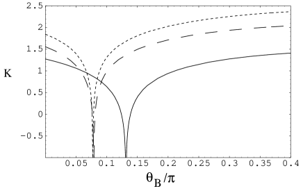
We see that the D-brane model give rise to a soft breaking pattern uniquely different from what is seen in SUGRA GUT models. Thus it would be difficult to find a GUT group breaking where $\tilde{m}_{1}=\tilde{m}_{3}\neq\tilde{m}_{2}$ and and similarly the above pattern of sfermion and Higgs soft masses. Brane models can achieve the above pattern since they have the freedom of associating different parts of the SM gauge group with different branes. In particular, the fact that the $\tilde{m}_{1}$ amd $\tilde{m}_{3}$ phases are equal causes cancelation between the gluino and neutralino EDM diagrams, and considerably aids in satisfying the EDM constraints. Fig.8 exihibits this phenomena where K is plotted as a function of $\theta_{B}$ for $d_{e}$ for tan$\beta$=2 (solid), 5 (dashed), 10 (dotted) with phases $\phi_{1}=\phi_{3}=\pi+\alpha_{0A}=-1.25\pi$ and $m_{3/2}=150$ GeV, $\theta_{b}=0.2$, $\Theta_{1}$=0.85. One sees that $\theta_{B}$ can be quite large and still satisfy the EDM bound $K\leq$0, i.e. $\theta_{B}\simeq 0.4$ for tan$\beta$=2 and $\theta_{B}\simeq 0.25$ even for tan$\beta$=10. If one reduces the gaugino phases, e.g. to $\alpha_{1}=\alpha_{3}=-1.1\pi$, one finds $\theta_{B}<0.2$ showing that the enhanced values of $\theta_{B}$ are indeed due to the cancellations allowed by the gaugino phases.

While $\theta_{B}$ can be relatively large at the electroweak scale, one finds as in the mSUGRA models, $\theta_{0B}$ at the GUT scale is large (when $\alpha_{1}=\alpha_{3}=\pi+\alpha_{0A}$ is large) but must be fine tuned, i.e. the allowed range $\Delta\theta_{0B}$ is small unless tan$\beta$ is small. This is illustrated in Fig.9 where $\Delta\theta_{0B}$ is plotted as a function of tan$\beta$. For these parameters ($\alpha_{0A}=-\pi/4$) there is already a 1 $\%$ finetuning in $\theta_{0B}$ at tan$\beta$=5, with increased fine tuning required for higher tan$\beta$. Thus this class of D-brane models does not resolve the fine tuning problem.

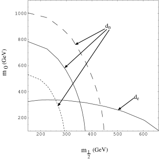
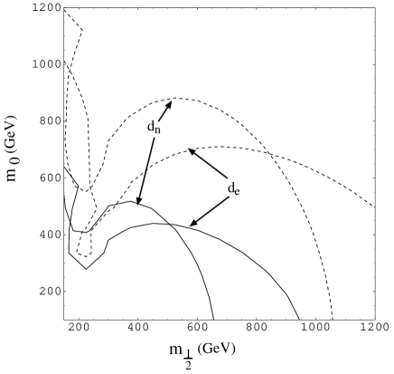
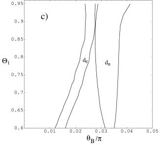
While as discussed in Sec.2 there are uncertainties in the calculation of the neutron EDM, it is of interest to see what parts of the parameter space remains if one requires that the experimental EDM constraint is satisfied simultaneously for $d_{e}$ and $d_{n}$. (We assume here the validity of the calculations of $d_{n}$ described in sec.2) An example of this is shown in Fig.10 where the allowed regions for $d_{e}$ and $d_{n}$ are shown for $\phi_{1}=\phi_{3}=\pi-\alpha_{0A}$=-1.90$\pi$ for different tan$\beta$. One sees that the overlap where the $d_{e}$ and $d_{n}$ EDM constraints are simultaneously satisfied disappears for tan$\beta>5$ for these parameters. Note also that while $d_{n}$ can tolerate larger $\theta_{B}$, to have both EDM constraints satisfied requires $\theta_{B}\stackrel{{\scriptstyle<}}{{\sim}}0.15$ in this example. In general, the overlap region broadens in $\Theta_{1}$ the closer $\phi_{1}=\phi_{3}$ is to $-2\pi$ (i.e. real $\tilde{m}_{1}=\tilde{m}_{3}$), but the allowed $\theta_{B}$ then becomes smaller (since the amoumnt of neutralino-gluino cancelation is reduced).

4 Models with small phases

Both the SUGRA and D-brane models posseses a serious fine tuning problem at $M_{G}$ in $\theta_{0B}$ when phases are large unless tan$\beta$ is small. For models of this type “naturalness” is to be defined at $M_{G}$, and one might ask whether in fact models might exist where all the phases are naturally small, e.g. $O(10^{-2})$, thus resolving the EDM problem. We present now one such possibility.

Below the compactification sacle $M_{c}$, one may analyse a model in terms of the supergravity functions of the chiral fields $\phi_{\alpha}$: the gauge kinetic function $f_{ij}(\phi_{\alpha})$, the Kahler potential $K(\phi_{\alpha},\phi_{\alpha}^{\dagger})$ and the superpotential $W(\phi_{\alpha})$. While the origin of supersymmetry breaking remains unknown, one may characterize it by assuming the existence of a hidden sector where some fields, e.g. moduli or dilaton, grow VEVs of Planck mass size:

$$x_{i} = \kappa<\Phi_{i}>=O(1).$$ (34)

Here $\kappa^{-1}=M_{Pl}=2.4\cdot 10^{18}$ GeV. We write $\{\Phi_{\alpha}\}=\{\Phi_{i},\Phi_{a}\}$ where $\Phi_{a}$ are the physical sector fields and expand the Kahler potential in a power series of the physical fields:

$$K = \kappa^{-2}c^{(0)}+(c_{ab}^{(2)}\Phi_{a}\Phi_{b}+{1\over M}c_{abc}^{(3)}\Phi_{a}\Phi_{b}\Phi_{c}+...)+(\tilde{c}_{ab}^{(2)}\Phi_{a}\Phi_{b}^{{\dagger}}$$

$$+ {1\over M}\tilde{c}_{abc}^{(3)}\Phi_{a}^{{\dagger}}\Phi_{b}\Phi_{c}+...)$$

where $M$ is a large mass. The $c^{(i)},\tilde{c}^{(i)}$ are dimensionless functions of $x_{i}$ and are assumed to be $O(1)$. The first parenthesis is holomorphic and hence can be transferred to the superpotential by a Kahler transformation:

$$W\rightarrow W+\kappa^{2}W(c_{ab}^{(2)}\Phi_{a}\Phi_{b}+{1\over M}c_{abc}^{(3)}\Phi_{a}\Phi_{b}\Phi_{c}+...)$$ (36)

The leading terms on the right arise when $W$ is replaced by its VEV after SUSY breaking, ($\kappa^{2}<W>\simeq m_{3/2}$) and one of the cubic terms (e.g. $\Phi_{c}$) has a GUT scale VEV arising e.g. from the GUT group breaking to the Standard Model, $<\Phi_{c}>\simeq M_{G}$. This then gives rise to the $\mu$ term, $W\rightarrow W+\mu_{ab}\Phi_{a}\Phi_{b}$, where

$$\mu_{ab} = (c_{ab}^{(2)}+{M_{G}\over M}c_{abc}^{(3)})m_{3/2}.$$ (37)

If one assumes now that the renormalizable terms $c^{(2)}_{ab}$ in $K$ is real, $c^{(3)}_{abc}$ is complex but with arbitrary size phase, $\mu^{0}$ will grow a phase $\theta_{0\mu}$ of size $M_{G}/M$ for $M>>M_{G}$ without any fine tuning. For SUGRA models one expects $M=M_{\rm Pl}$ and hence $\theta_{0\mu}\simeq O(10^{-2})$. Similar results can occur for the phases in the soft breaking parameters and one might have a model where all phases are $O(10^{-2})$ naturally suppressing the EDMs without any fine tuning. For D-brane models considered here one expects $M=M_{\rm str}$ and as discussed in Sec III, $M_{\rm str}\cong 8\times 10^{16}$ leading to phases of size $O(10^{-1})$. There is then a partial suppression of the EDMs leading perhaps to interesting predictions for the next round of EDM measurements for such models.

5 CONCLUSIONS

The very strong experimental constraints on the electron and neutron electric dipole moments put additional constraints on the parameter space of the SUSY models if the mass spectrum lies below $\sim$ 1 TeV. We have studied this within the framework of models where the physics is determined at a high scale (e.g. GUT or Planck scale). For SUGRA GUT models the renormalization group equation naturally suppress $\alpha_{t}$, the $A_{t}$ phase at the electroweak scale, due to the nearness of the t-quark Landau pole and so the phase $\alpha_{0A}$ at $M_{G}$ can be naturally large, even $\pi/2$, and still lead to acceptable EDMs. The possible cancelations of different parts of the EDM amplitudes does allow $\theta_{B}$, the B phase at the electroweak scale, to be large, i.e. $O(10^{-1})$ when $\alpha_{0A}=O(1)$, but only for low tan$\beta$ i.e. tan$\beta\leq$3. The combined conditions of the experimental EDM constraints and the requirement of radiative breaking of $SU(2)\times U(1)$ then leads to $\theta_{0B}$ to be $O(1)$ at the $M_{G}$ and very tightly determined for tan$\beta\stackrel{{\scriptstyle>}}{{\sim}}3$. Thus there is a new fine tuning problem at $M_{G}$ unless tan$\beta$ is small. We note that LEP data already requires tan$\beta>2$, and the RUN II at the Tevatron will be able to probe higher tan$\beta$ as it searches for the Higgs.

For a class of D brane models arising in Type IIB orientifolds, one can have the gaugino mass phases obey $\phi_{1}=\phi_{2}\neq\phi_{3}$ allowing $\theta_{B}$ to become larger due to additional cancelations between gluino and neutralino diagrams. However, the same fine tuning problem for $\theta_{0B}$ at $M_{G}$ arises unless tan$\beta$ is small. Further, one needs tan$\beta\stackrel{{\scriptstyle<}}{{\sim}}5$ to get a significant overlap between the allowed $d_{e}$ and $d_{n}$ regions in parameter space when the $\phi_{i}$ are large.

The fact that the fine tuning problem of $\theta_{0B}$ appears to be endemic leads one to consider the possibility that all phases might naturally be small at $M_{G}$. A simple model showing this might arise where the phases $\phi_{i}=O(M_{G}/M)$ is discussed, where $M=M_{\rm Planck}$ for SUGRA models and $M=M_{\rm string}$ for D-brane models.

6 Acknowledgement

This work was supported in part by National Science Foundation Grant No. PHY-9722090.

Figure 1: Diagrams contributing to $d_{f}$. For f=q(l) the scalars are $\tilde{q}(\tilde{l})$ and gauginos are $\tilde{\chi}^{0}_{i}$, $\tilde{\chi}^{\pm}_{i}$, $\tilde{g}$ where $\tilde{\chi}^{\pm}_{i}$, i=1,2 are charginos and $\tilde{\chi}^{0}_{i}$, i=1…4 are neutralinos.

Figure 2: Two loop Barr-Zee diagrams where A is the CP odd Higgs and $\tilde{q}_{i}$ are the mass diagonal squark states.

Figure 3: Two loop Weinberg type diagram.

Figure 4: K vs $m_{0}$ for $d_{e}$ (electron EDM) for tan$\beta=3$ (solid), 10 (dashed) and 20 (dotted) respectively for $m_{1/2}=300$, $|A_{0}|=300$ GeV, $\alpha_{0A}={\pi\over 2}$, $\theta_{B}=$0.02.

Figure 5: $\theta_{0B}$ vs $m_{1/2}$. Upper and lower lines are the allowed range so that $K\leq 0$. The solid lines are for $d_{n}$ and the dotted lines are for $d_{e}$.

Figure 6: The K=0 contours are plotted as a function of $m_{0}$ and $m_{1/2}$. The dotted, solid and dashed lines are for $m_{d}$ (1 GeV)=5, 8 and 12 MeV respectively. The other input parameters are $\alpha_{0A}={\pi\over 2}$, $|A_{0}|=300$ GeV $\theta_{B}$=0 and tan$\beta$=3. Excluded regions are below $d_{e}$ and to the left of $d_{n}$ curves.

Figure 7: Allowed region in $m_{0}-m_{1/2}$ plane for $d_{e}$ and $d_{n}$. The other input parameters are $\alpha_{0A}={\pi\over 2}$, $|A_{0}|=300$ GeV, $\theta_{B}$=0 and tan$\beta$=20. The solid lines are for K=0 and the dotted lines are for K=-0.5.

Figure 8: K vs. $\theta_{B}$ for $d_{e}$ for $\phi_{1}$=$\phi_{3}$=$\pi+\alpha_{0A}$=-1.25$\pi$, $m_{3/2}$=150 GeV, $\theta_{b}$=0.2, $\Theta_{1}=0.85$, with tan$\beta$=2(solid), 5(dashed), 10(dotted).

Figure 9: Values of $\Delta\theta_{0B}$ for $d_{e}$ satisfying the EDM constraint as a function of tan$\beta$. Parameters are as in Fig.8.

Figure 10: Allowed regions for $d_{e}$ and $d_{n}$ for $\theta_{b}$=0.2, $m_{3/2}$=150 GeV and $\phi_{1}$=$\phi_{3}$=-1.90$\pi$, for a) tan$\beta$=2, b) tan$\beta$=3 and c) tan$\beta$=5.