Thermal Field Theory in Equilibrium

Abstract

In this talk, I review recent developments in equilibrium thermal field theory. Screened perturbation theory and hard-thermal-loop perturbation theory are discussed. A self-consistent $\Phi$-derivable approach is also briefly reviewed.

1 Introduction

Thermal field theory has applications in many areas of physics and one of those is the early Universe. There is an excess of matter over antimatter in the present Universe. Unless this was an initial condition in the Big Bang Scenario, this baryon asymmetry must have been created during the evolution of the Universe. According to Sakarov’s three criteria for baryogenesis, the Universe must have been out of equilibrium, there must be baryon-number violating processes, and there must be CP violation. Although baryon-number violating processes are exponentially suppressed at $T=0$, they are significant at high temperatures. Moreover, CP violation is known from the kaon system, and the Universe was out of equilibrium during a cosmological phase transition if it was first order. Hence, all the necessary ingredients of baryosynthesis may have been present in the early Universe and has been subject of intense investigation in recent years.

Another important application of thermal field theory is heavy-ion collisions. QCD is expected to undergo a phase transition at high temperature and/or high density, where chiral symmetry is restored, and quarks and gluons are deconfined. Hadrons are no longer the relevant degrees of freedom, but matter is described in terms of a plasma of interacting quarks and gluons. A quark-gluon plasma is expected to be created in heavy-ion collisions at RHIC and LHC. Signatures of the formation of a quark-gluon plasma includes photon and dilepton production, and $J/\psi$ suppression,

In order to understand such complicated nonequilibrium phenomena, we need to have equilibrium field theory under control. In this talk, I would like to give an overview of recent developments in equilibrium thermal field theory.

2 Weak-coupling Expansion

Let us start the discussion by considering a massless scalar field theory with a $\phi^{4}$ interaction. The Euclidean Lagrangian is

$${\cal L} = {1\over 2}(\partial_{\mu}\Phi)^{2}+{g^{2}\over 24}\Phi^{4}\;.$$ (1)

Using ordinary perturbation theory, one splits ${\cal L}$ into a a free part (quadratic piece) and treats the $\phi^{4}$ term as an interaction. The loop expansion is then an expansion in powers of $g^{2}$ around an ideal massless gas. However, it is well known that naive perturbation theory breaks down beyond two-loop order due to infrared divergences since the scalar field is massless, and that one needs to reorganize the perturbative expansion. Physically, the infrared divergences are screened due to a thermally generated mass of order $gT$.

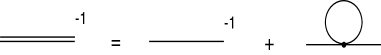
Figure 1: Two-point function in the one-loop approximation.

In order to incorporate the physics of Debye screening, we need to use an effective propagator that includes the mass. Using the effective propagator in a one-loop calculation is equivalent to summing all the bubble diagrams of Fig. 2.

Figure 2: Summation of bubble diagrams using a dressed propagator.

The summation of the bubble diagrams gives a contribution to the free energy of order $g^{3}$, and is thus nonanalytic in $g^{2}$. The resummation of diagrams can be made into a systematic expansion in powers of $g$. The free energy has been calculated through order $g^{5}$ in the weak-coupling expansion [1]:

$${\cal F}={\cal F}_{\rm ideal}\left[1-{5\over 4}\left({g\over 4\pi}\right)^{2}+{5\sqrt{6}\over 3}\left({g\over 4\pi}\right)^{3}+{3\over 2}\left({g\over 4\pi}\right)^{4}\right.\left.+\left(24.5\log{g\over 4\pi}+13.2\right)\left({g\over 4\pi}\right)^{5}\right]\;,$$ (2)

where ${\cal F}_{\rm ideal}=-(\pi^{2}/90)T^{4}$, and the renormalization scale $\mu_{4}=2\pi T$. It turns out that the weak-coupling expansion does not converge unless the coupling is tiny. This lack of convergence is not specific to $\phi^{4}$ theory but occurs also in QCD [1]. In QCD, the $g^{3}$ term is smaller than the $g^{2}$ term in the free energy only if $\alpha_{s}\sim 1/20$. This corresponds to a temperature of $10^{5}$ GeV, which is many orders of magnitude larger than the temperatures expected in heavy-ion collisions (approximately 0.5 GeV at RHIC).

3 Screened Perturbation Theory

There are several ways of reorganizing perturbation theory to improve its convergence properties. One of the most successful approaches is “screened perturbation theory” developed by Karsch, Patkós, and Petreczky [2]. A local mass term is added to and subtracted from the Lagrangian, with the added mass term treated nonperturbatively, and the subtracted term as a perturbation. Thus the Lagrangian is split according to

$${\cal L}_{\rm free} = {1\over 2}(\partial_{\mu}\phi)^{2}+{1\over 2}m^{2}\phi^{2}\;,$$ (3)

$${\cal L}_{\rm int} = {g^{2}\over 24}\phi^{4}-{1\over 2}m^{2}\phi^{2}\;.$$ (4)

Hence, screened perturbation theory is essentially expanding around an ideal gas of massive particles. A straightforward calculation give the renormalized one-loop free energy in screened perturbation theory:

$${\cal F_{\rm SPT}} = {1\over 2}T\sum_{n=-\infty}^{\infty}\int{d^{3-2\epsilon}k\over(2\pi)^{3-2\epsilon}}\log\left({\omega_{n}^{2}+k^{2}+m^{2}}\right)$$ (5)

$$= {T\over 2\pi^{2}}\int_{0}^{\infty}dk\;k^{2}\log\left(1-e^{-\beta\omega}\right)+{m^{4}\over 32\pi^{2}}\left[{3\over 4}+\log{\mu\over m}\right]\;,$$

where $\omega_{n}=2\pi T$ are the Matsubara frequencies and $\mu$ is a renormalizaton scale associated with dimensional regularization.

At this point I would like to emphasize that the screening mass $m$ is a completly arbitrary parameter. To complete a calculation using screeened perturbation theory, one must specify how $m$ is determined. Karsch et al. [2] used a one-loop gap equation to determine the screening mass:

$$m^{2}(T)={g^{2}\over 4\pi^{2}}\int_{0}^{\infty}dk\;{k\over e^{\beta\omega}-1}\;,\hskip 28.45274pt{\rm where}\;\;\omega=\sqrt{k^{2}+m^{2}}\;.$$ (6)

Figure 3: Comparison of screened perturbation theory (SP) and the weak-coupling expansion (P).

In Fig. 3, we show the weak-coupling expansions through order $g^{2}$ (lower curve) and order $g^{3}$ (upper curve) normalized to ${\cal F}_{\rm ideal}$. The two approximations to the free energy have different signs and show the lack of convergence of the weak-coupling expansion. The two curves that are almost on top of each other are the one and two-loop approximations in screened perturbation theory, with the mass parameter determined from Eq. (6). We conclude that screened perturbation theory has good convergence properties for a wide range of values for the coupling constant $g$.

4. HTL Perturbation Theory

We would like to generalize screened perturbation theory to gauge theories. We cannot simply add and subtract a local mass term in the Lagrangian since this would violate gauge invariance. However, there is a way to incorporate plasma effects, including propagation of massive quasiparticles, screening of interactions and Landau damping and still maintain gauge invariance. This approach is hard-thermal-loop (HTL) perturbation theory, and involves effective propagators and effective vertices [3, 4].

The free energy of pure-glue QCD to leading order in HTL perturbation theory is

$${\cal F}=8\left[(d-1){\cal F}_{T}+{\cal F}_{L}+\Delta{\cal F}\right]\,,$$ (7)

where $d=3-2\epsilon$, ${\cal F}_{T}$ and ${\cal F}_{L}$ are the transverse and longitudinal contributions to the free energy, respectively, and $\Delta{\cal F}$ is a counterterm. In the imaginary-time formalism, we have

$${\cal F}_{T} = {1\over 2\beta}\sum_{n}\int_{k}\log\left[k^{2}+\omega_{n}^{2}+\Pi_{T}(\omega_{n},k)\right]\;,\hskip 28.45274pt$$ (8)

$${\cal F}_{L} = {1\over 2\beta}\sum_{n}\int_{k}\log\left[k^{2}-\Pi_{L}(\omega_{n},k)\right]\,,$$ (9)

where the transverse and longitudinal self-energy functions are

$$\Pi_{T} = -{3\over 2}m_{g}^{2}{\omega_{n}^{2}\over k^{2}}\left[1-{\omega^{2}_{n}+k^{2}\over 2i\omega_{n}k}\log{i\omega_{n}+k\over i\omega_{n}-k}\right]\;,$$ (10)

$$\Pi_{L} = 3m_{g}^{2}\left[{i\omega_{n}\over 2k}\log{i\omega_{n}+k\over i\omega_{n}-k}-1\right]\;.$$ (11)

The sum over the Matsubara frequencies $\omega_{n}=2\pi nT$ can be rewritten as a contour integral around a contour $C$ that encloses the points $\omega=i\omega_{n}$. The integrand has branch cuts that start at $\pm\omega_{T}(k)$ and $\pm\omega_{L}(k)$, where $\omega_{T}(k)$ and $\omega_{L}(k)$ are the dispersion relations for transverse and longitudinal gluon quasiparticles, respectively. The integrand also has a branch cut running from $\omega=-k$ to $\omega=k$ due to the functions $\Pi_{T}$ and $\Pi_{L}$. The contour can be deformed to wrap around the quasiparticle and Landau-damping branch cuts. Some of the temperature-independent integrals over $\omega$ can be calculated analytically, while others must be evaluated numerically. With dimensional regularization, the logarithmic ultraviolet divergences show up as poles in $\epsilon$. Using the modified minimal subtraction ($\overline{\mbox{MS}}$) renormalization prescription with the counterterm $\Delta{\cal F}=9m^{4}_{g}/64\pi^{2}\epsilon$, we obtain

$${\cal F}_{\rm HTL} = {8\over\pi^{2}}T\int^{\infty}_{0}k^{2}dk\log(1-e^{-\beta\omega_{T}})+{4\over\pi^{2}}T\int^{\infty}_{0}k^{2}dk\log{1-e^{-\beta\omega_{L}}\over 1-e^{-\beta k}}+{1\over 2}\;m_{g}^{2}T^{2}$$ (12)

$$-{8\over\pi^{3}}\int^{\infty}_{0}d\omega\;n(\omega)\int^{\infty}_{\omega}k^{2}dk\left[2\phi_{T}-\phi_{L}\right]+{9\over 8\pi^{2}}\;m_{g}^{4}\;\left[\log{m_{g}\over\mu_{3}}+0.31\right]\,.$$

Here, $\omega_{T}$ and $\omega_{L}$ are the transverse and longitudinal dispersion relations which are the solutions to $k^{2}-\omega_{T}^{2}+\Pi_{T}(-i\omega_{T},k)=0$, and $k^{2}-\Pi_{L}(-i\omega_{L},k)=0$. Moreover, $n(\omega)$ is the Bose-Einstein distribution function and the angles $\phi_{T}$ and $\phi_{L}$ satisfy

$${3\pi\over 4}m^{2}_{g}{\omega(k^{2}-\omega^{2})\over k^{3}}\cot\phi_{T} = k^{2}-\omega^{2}\;+\;{3\over 2}m^{2}_{g}{\omega^{2}\over k^{2}}\left[1+{(k^{2}-\omega^{2})\over 2k\omega}\log{k+\omega\over k-\omega}\right]\;,$$ (13)

$${3\pi\over 2}m_{g}^{2}{\omega\over k}\cot\phi_{L} = k^{2}\;+\;3m_{g}^{2}\left[1-{\omega\over 2k}\log{k+\omega\over k-\omega}\right]\;.$$ (14)

Figure 4: HTL pressure for pure-glue QCD as a function of $T/T_{c}$. Lattice results from Ref. [5].

The leading-order HTL result for the pressure is shown in Fig. 4 as the shaded band that corresponds to varying the renormalization scales $\mu_{3}$ and $\mu_{4}$ by a factor of two around their central values $\mu_{3}=0.717m_{g}$ and $\mu_{4}=2\pi T$. This value of $\mu_{3}$ is chosen in order to minimize the pathological behavior of ${\cal F}_{HTL}$ at low temperatures [4]. We also show as dashed curves the weak-coupling expansions through order $\alpha_{s}$, $\alpha_{s}^{3/2}$, $\alpha_{s}^{2}$, and $\alpha_{s}^{5/2}$ labelled 2, 3, 4, and 5. We have used a parameterization of the running coupling constant $\alpha_{s}(\mu_{4})$ that includes the effects of two-loop running With the above choices of the renormalization scales, our leading-order result for the HTL free energy lies below the lattice results of Boyd et al. [5] (shown as diamonds) for $T>2T_{c}$. However, the deviation from lattice QCD results has the correct sign and roughly the correct magnitude to be accounted for by next-to-leading order corrections in HTL perturbation theory [4]. Comparing the weak-coupling expansion with the the high-temperature expansion of (12), and identifying $m_{g}^{2}$ with its weak-coupling limit ${4\pi\over 3}\alpha_{s}T^{2}$, we conclude that HTL perturbation theory overincludes the $\alpha_{s}$ contribution by a factor of three [4]. The $\alpha_{s}^{3/2}$ contribution which is associated with Debye screening is included correctly. At next-to-leading order, HTL perturbation theory agrees with the weak-coupling expansion through order $\alpha_{s}^{3/2}$. Thus the next-to-leading order contribution to ${\cal F}/{\cal F}_{\rm ideal}$ in HTL perturbation theory will be positive at large $T$ since it must approach $+{15\over 2}\alpha_{s}/\pi$.

4 Self-consistent $\Phi$-derivable Approach

An alternative to screened perturbation theory is the self-consistent $\Phi$-derivable approach [6]. The free energy can be expressed as the stationary point of the thermodynamic potential $\Omega[D]$.

$$\beta\Omega[D] = {1\over 2}{\rm Tr}\log D^{-1}-{1\over 2}\Pi D+\Phi[D]\;,$$ (15)

where $D$ is the exact propagator and $\Phi[D]$ is given by the sum of two-particle irreducible diagrams. the condition that $\Omega[D]$ be a statinary point gives an integral equation for the propagator:

$${\partial\Phi[D]\over\partial D}={1\over 2}\Pi\;.$$ (16)

The free energy ${\cal F}$ is obtained by solving the integral equation for $D$ and inserting the solution into the the thermodynamics potential $\Omega[D]$. Blaizot et al. [7] have developed a HTL approximation to the $\Phi$-derivable approach and applied it to both scalar theory and nonabelian gauge theories.

I do not have enough time to discuss this approach in depth and compare it critically with screened perturbation theory and HTL perturbation theory, but I will mention a few key points:

• The $\Phi$-derivable approach is thermodynamically consistent, which means that the usual thermodynamic relations between pressure, energy density and entropy hold exactly. Thermodynamic consistency is destroyed by the HTL approximation of Ref. [7]. It holds only up to perturbative corrections in screened perturbation theory and HTL perturbation theory.

• The $\Phi$-derivable free energy is gauge dependent since only the propagator and not the vertices are dressed. This problem is avoided in the HTL approximation of Tef [7] by not solving the gap equation with sufficient accuracy the see the gauge dependence. HTL perturbation theory is gauge-fixing independent by construction.

• The running of the coupling constant in the $\Phi$-derivable approach is not consistent with the $\beta$ function of the theory. In Ref [7], the correct running is put in by hand.

Higher-order calculations using the self-consistent $\Phi$-derivable approach are currently being carried out for the scalar theory by Braaten and Petitgirard [8].

5 Summary

The weak-coupling expansion is useless for temperatures which are relevant for experiments at RHIC and LHC. We have seen that screened perturbation theory shows good convergence for a large range of values for the coupling $g$. This fact gives us hope that HTL perturbation theory might be a useful framework for calculating static and dynamical quantities of a quark-gluon plasma at experimentally accessible energies. A next-to-leading order calculation of the free energy using HTL perturbation theory is currently being carried out [9].

References

- [1] P. Arnold and C. Zhai, Phys. Rev. D50, 7603 (1994); Phys. Rev. D51, 1906 (1995).
- [2] F. Karsch, A. Patkós, and P. Petreczky, Phys. Lett. B401, 69 (1997).
- [3] E. Braaten and R.D. Pisarski, Phys. Rev. Lett. 64, 1338 (1990); Nucl. Phys. B337, 569 (1990).
- [4] J. O. Andersen, E. Braaten and M. Strickland, Phys. Rev. Lett. 83, 2139 (1999); Phys Rev. D61, 014017 (1999); hep-ph/9908323.
- [5] G. Boyd et al., Phys. Rev. Lett. 75 4169 (1995); Nucl. Phys. B469 419 (1996).
- [6] J. M. Luttinger and J. C. Ward, 118, 1417 (1960); G. Baym, Phys. Rev. 127, 1391 (1962).
- [7] J.-P. Blaizot, E. Iancu and A. Rebhan, Phys. Rev. Lett. 83 (1999), hep-ph/9910309.
- [8] E. Braaten and E. Petitgirard, in preparation.
- [9] J. O. Andersen, E. Braaten and M. Strickland, in preparation.