TAUP 2618/00

The Components of the ${\mathbf{\gamma}^{*}\gamma^{*}}$ Cross Section

E.  G O T S M A N ${\!}^{\mbox{\scriptsize 1)}}$, E.  L E V I N ${\!}^{\mbox{\scriptsize 2)}}$,
U.  M A O R ${\!}^{\mbox{\scriptsize 3)}}$ and E.  N A F T A L I ${\!}^{\mbox{\scriptsize 4)}}$

School of Physics and Astronomy
Raymond and Beverly Sackler Faculty of Exact Science
Tel Aviv University, Tel Aviv, 69978, ISRAEL

Abstract: We extend our previous treatment of $\gamma^{*}$p cross section based on Gribov’s hypothesis to the case of photon-photon scattering. With the aid of two parameters, determined from experimental data, we separate the interactions into two categories corresponding to short (”soft”) and long (”hard”) distance processes. The photon-photon cross section, thus, receives contributions from three sectors, soft-soft, hard-hard and hard-soft. The additive quark model is used to describe the soft-soft sector, pQCD the hard-hard sector, while the hard-soft sector is determined by relating it to the $\gamma^{*}$p system. We calculate and display the behaviour of the total photon-photon cross section and it’s various components and polarizations for different values of energy and virtuality of the two photons, and discuss the significance of our results.

1 Introduction

Scattering in the high energy (low $x$) limit has been studied in perturbative QCD (pQCD) over the past few years, mainly through the analysis of deep inelastic (DIS) events of lepton-hadron and hadron-hadron collisions. Such pQCD investigation requires some knowledge of the non perturbative contribution which is introduced, through the initial input to the evolution equations or put in explicitly. In this paper we present a study of virtual photon-photon scattering. Our investigation is based on our model for $\gamma^{*}$p cross section [1] , which provides the framework for the present calculation. Our goal is two fold:

1. In any QCD process, finding the dynamics for intermediate distances is still an open problem, as it involves a transition between short distance (“hard” - perturbative) and large distance (“soft” - non perturbative) physics. In Ref. [1] we have suggested a procedure, based on Gribov’s general approach [2], of how to accommodate both contributions in DIS calculations. Two photon physics is an obvious reaction where these ideas can be further studied and re-examined.

2. Virtual photon-photon scattering has been proposed [3, 4, 5, 6] as a laboratory to study the BFKL Pomeron [7], as the total cross section of two highly virtual photons provides a probe of BFKL dynamics. Our study enables one to estimate the background to the proposed BFKL process. This background consists of two contributions: ($i$) We give an explicit estimate of the soft component in $\gamma^{*}\gamma^{*}$ scattering. ($ii$) Our pQCD estimate for the hard component is based on DGLAP [8] and as such can be used to assess when the BFKL dynamics start to dominate.

Impressive attempts have been made [9, 10] to describe two photon physics within the framework of Vector Dominance Model (VDM) mainly as a soft interaction. However, one can consider a two photon interaction as an interesting tool for investigating the interplay between soft and hard physics [11]. The photon can appear as an unresolved object or as a perturbative fluctuation into an interacting quark-antiquark system. A careful analysis of the various components of the total cross section will help us understand the interface of the short distance and large distance interaction.

In $e^{+}e^{-}$ colliders, the measurement of the $\gamma^{*}\gamma^{*}$ is carried out by double tagging the outgoing leptons close to the forward direction, as most of the initial energy is taken by the scattered electrons. The double tagged cross section falls off with the increase of the photons virtualities due to the photon propagator. The experimental statistics are improved for single and no tag events where one of the colliding photons or both are quasi-real [12]. There is, therefore, a theoretical interest and an experimental need to better understand and estimate the perturbative and non-perturbative contributions with realistic configurations of the two photon virtualities.

Our paper deals with photon-photon collisions in the high energy limit, which confines us to low $x$ values. A pQCD investigation of $e\gamma$ DIS is non trivial [13] due to the dual nature of the photon target (quasi-real or virtual) which can be perceived as either a hadron like partonic system or a point like object. The resulting difficulties in pQCD calculations of $F_{2}^{\gamma}$ in the small $x$ limit have been extensively discussed in the literature and several strategies have been devised to bypass these problems [13]. For the purpose of our analysis we follow the approach suggested by Glück and Reya [14] in which the pQCD calculations has no predictive power regarding the normalization of $F_{2}^{\gamma}$ but it retains, as for a proton target, the $\alpha_{\rm S}$ dependence of the evolution equations.

The above philosophy is very appropriate for our program where we distinguish between the hard pQCD mode and the non-perturbative QCD (npQCD) soft mode of the gluon fields by introducing [1, 15], two separation parameters ($M^{2}_{0,T}$ and $M^{2}_{0,L}$) in which we match the long and short distance components of the transverse (T) and longitudinal (L) contributions to the total $\gamma^{*}\gamma^{*}$ cross-section. Our ideology is close to the Semiclassical Gluon Field Approach developed in Ref. [16]. This approach allows one to find a relation between scattering amplitudes and the property of the QCD vacuum based on the Model of the Stochastic Vacuum (MSV) [17]. Whereas the MSV is guided by the assumption of a microscopic structure of the QCD vacuum, our model is phenomenologically oriented based on the Additive Quark Model (AQM)[18]. The MSV has been combined [11] with the two Pomeron model [19]. In the two Pomeron model the hard Pomeron is a fixed $J$-pole whose $Q^{2}$ dependence is determined by fitting to data. In a pQCD calculation of the hard Pomeron, one has an effective $J$-pole whose dependence on $x$ and $Q^{2}$ is determined by $xG(x,Q^{2})$. A short review of the various approaches to $\gamma^{*}\gamma^{*}$ reactions at high energies, stressing the need for a simultaneous determination of both the soft and the hard contributing components, has just appeared [20].

The plan of our paper is as follows: In section 2 we review the generalization of the ideas presented in Ref. [1] and outline the expansion of this model for the $\gamma^{*}\gamma^{*}$ cross section. In section 3 we derive the complete set of formulae for the total cross section components. We present the details of our numerical calculations in section 4 and compare our results with the high energy experimental data available to date. Our conclusions are summarized in section 5.

2 Review of the Approach

Our approach follows from the ideas presented in Refs. [21]. This was first suggested in Ref. [15] and successfully applied in Ref. [1].

According to Gribov’s general approach [2], the interaction of a virtual photon, in any QCD description, can be interpreted as a two stage process. The first stage is the fluctuation of the photon into a hadronic system, and in the next stage the hadronic system interacts with the “target”, which in our case is another hadronic system from a different parent photon (see Fig. 1). These two processes are time ordered and can be treated independently. The vertex function $\Gamma(M^{2})$ of the photon fluctuation into a $q\bar{q}$ pair of mass $M$ is given by the experimental value of the ratio

$$\Gamma(M^{2})=R(M^{2})=\frac{\sigma(e^{+}e^{-}\rightarrow\mbox{hadrons})}{\sigma(e^{+}e^{-}\rightarrow\mu^{+}\mu^{-})}\,.$$ (1)

Figure 1: Gribov’s approach.

The complete process of two virtual photons fluctuating into two quark-antiquark pairs which then interact with each other, can be expressed by the following dispersion relation:

$$\sigma(\gamma^{*}\gamma^{*}) = \left(\frac{\alpha_{\rm em}}{3\pi}\right)^{2}\int dM^{2}_{1}\>dM^{2}_{2}\>dM^{\prime 2}_{1}\>dM^{\prime 2}_{2}\frac{\Gamma(M^{2}_{1})}{\left(Q^{2}_{1}+M^{2}_{1}\right)}\frac{\Gamma(M^{2}_{2})}{\left(Q^{2}_{2}+M^{2}_{2}\right)}\times$$ (2)

$$\hskip 142.26378pt\sigma(M^{2}_{1},M^{\prime 2}_{1};M^{2}_{2},M^{\prime 2}_{2};s)\frac{\Gamma(M^{\prime 2}_{1})}{\left(Q^{2}_{1}+M^{\prime 2}_{1}\right)}\frac{\Gamma(M^{\prime 2}_{2})}{\left(Q^{2}_{2}+M^{\prime 2}_{2}\right)}\,,$$

where $\sigma(M^{2}_{1},M^{\prime 2}_{1};M^{2}_{2},M^{\prime 2}_{2};s)$ is the cross section of the interaction between two hadronic systems with masses $M_{1}$ and $M_{2}$ before the interaction and $M^{\prime}_{1}$ and $M^{\prime}_{2}$ after the interaction.

We introduce a separation parameter in the mass integrations, which may be different for longitudinal and transverse polarized virtual photon ($M_{0,L}$ and $M_{0,T}$ respectively). For masses below this parameter, the process is soft, long range, and hence one cannot describe the produced hadron state as a $q\bar{q}$ pair. For masses above the separation parameter, the distances between the quark and antiquark are short, and $\sigma(M^{2}_{1},M^{\prime 2}_{1};M^{2}_{2},M^{\prime 2}_{2};s)$, which depends on the gluon structure function, can be calculated in pQCD.

The calculation of the two photon total cross section, according to our approach, is derived following the same concepts of the $\sigma(\gamma^{*}p)$ calculations. Each of the two photons can be soft or hard, and we shall derive the formulae on this basis. Without loss of generality, we shall consider the case in which one photon (say, the upper one) is “harder” than the other, hence there are three sectors of the calculation:

1. “Hard-hard” when both photons are hard. We treat the interaction between the two $q\bar{q}$ pairs in pQCD, calculating all the diagrams in which the upper $q\bar{q}$ pair are harder than the gluons in the ladder, and the gluons in the ladder are harder than the lower pair $k^{2}_{1}\gg\ell^{2}_{1}\gg\ell^{2}_{2}\gg k^{2}_{2}$ (see Fig. 2). The cross section of the interaction in the hard-hard sector can be expressed through $xG_{q}$, the distribution function of a gluon ladder emitted from a single quark.

   To find $xG_{q}$ we recall that, in the region of small $x$, the evolution equation has the form:

   $$\frac{d^{2}xG_{q}(x,Q^{2})}{d\log\frac{1}{x}d\log Q^{2}}=\frac{N_{c}}{\pi}\,\alpha_{S}(Q^{2})\,xG_{q}(x,Q^{2}).$$ (3)

   The solution of this equation in the DLLA has been already given in [22],

   $$xG_{q}(x,Q^{2})=G_{0}\,I_{0}\left(2\sqrt{\gamma(Q^{2})\log\frac{1}{x}}\right),$$ (4)

   with $G_{0}=0.0453$ and

   $$\gamma(Q^{2})=\frac{12N_{c}}{11N_{c}-2n_{f}}\log\left(\frac{\log\frac{Q^{2}}{\Lambda^{2}}}{\log\frac{Q^{2}_{0}}{\Lambda^{2}}}\right).$$ (5)

2. “Soft-soft” for two soft photons. As stated, this is the case where neither of the hadronic systems can be treated in pQCD. Here we use the AQM [18] in which the interaction cross-section $\sigma(M^{2}_{1},M^{\prime 2}_{1};M^{2}_{2},M^{\prime 2}_{2};s)$ is diagonal with respect to $M_{j}$ and $M^{\prime}_{j}\,(j=1,2)$.

3. “Hard-soft” for the case that the upper photon is hard and the lower photon is soft. This sector is related, up to factorization, to the hard interaction between a nucleon and a photon, as the lower system is treated non perturbatively, while the upper hadronic system is a $q\bar{q}$ pair with small transverse separation. Thus, the interaction cross section $\sigma(M^{2}_{1},M^{\prime 2}_{1};M^{2}_{2},M^{\prime 2}_{2};s)$ is not diagonal and can be expressed through a nucleon gluonic structure function $xG$, with a factor of $\frac{2}{3}$, to account for the fact that we replace the nucleon $|qqq\rangle$ state with a $|q\bar{q}\rangle$ state.

   As we shall see, our integrations require the knowledge of $xG(x,\ell^{2})$ where $\ell^{2}$ spans also over small values where the published parameterizations for $xG$ are not valid. We follow Refs. [23] and [1] and introduce an additional gluon scale $\mu^{2}$ and assume that the gluon structure function can be approximated linearly by $\frac{\ell^{2}}{\mu^{2}}xG\left(x,\mu^{2}\right)$. Thus, our approach has two scales, one separating the hard integration from the soft, which is related to the size of the quark-antiquark pair, and the gluon scale which is related to the size of the quark. For more details – see Refs. [1], [23], and [24].

In the next section, we derive explicitly the formulae for the three sectors described above, taking into account both transverse and longitudinal polarized photons in each sector. In our numerical calculations which are presented in section 4, the choice of our parameters are consistent with Ref. [1].

3 Formulae for the Total $\gamma^{*}\gamma^{*}$ Cross Section

Figure 2: Some of the diagrams which contribute to the pQCD calculations.

3.1 The “Hard-Hard” components

The pQCD calculation for the total cross section of two hard photons is illustrated in diagrams of the type shown in Fig. 2. We denote the production amplitude of the two systems of $q\bar{q}$, one from each “hard” photon, by ${\cal M}_{\lambda_{1}\lambda_{1}^{\prime}\lambda_{2}\lambda_{2}^{\prime}}$ where $\lambda_{1}\ldots\lambda_{2}^{\prime}$ are the helicities of the four quarks. We follow Refs.[1, 15, 25] and write ${\cal M}_{\lambda_{1}\lambda_{1}^{\prime}\lambda_{2}\lambda_{2}^{\prime}}$ in the form:

$${\cal M}_{\lambda_{1}\lambda_{1}^{\prime}\lambda_{2}\lambda_{2}^{\prime}}=\sqrt{N_{c}}\int\;d^{2}\mbox{\boldmath{$k$}}_{1}^{\prime}d^{2}z_{1}^{\prime}\int\;d^{2}\mbox{\boldmath{$k$}}_{2}^{\prime}d^{2}z_{2}^{\prime}{\cal T}_{1,2}\psi_{1}\psi_{2}$$ (6)

where ${\cal T}_{1,2}={\cal T}(k^{\prime}_{1},k_{1},k^{\prime}_{2},k_{2})$ is the transition amplitude of all the 16 possible diagrams of Fig. 2, $\psi_{j}=\psi_{j}(k_{j}^{\prime},z_{j}^{\prime})\,\,j=1,2$ are the wave functions of the $q\bar{q}$ inside the photons, and $z_{j}\;(1-z_{j})$ is the fraction of the energy of the $j$ photon that is carried by the quark(antiquark). Here and throughout this paper our momentum variables are defined as the two-dimensional transverse components of a four momentum, i.e. $k\equiv k_{\perp}$.

In the leading $\log(1/x)$ approximation $z=z^{\prime}$ and therefore the transition amplitude ${\cal T}_{1,2}$ does not dependent on $z_{j},z_{j}^{\prime}$. In the limit where $k_{1}\gg\ell_{1}\gg\ell_{2}\gg k_{2}$ we write:

$${\cal T}_{1,2}=i\frac{4\pi s}{2N_{c}}\int\frac{d^{2}\mbox{\boldmath{$\ell$}}_{1}}{\ell^{2}_{1}}\int\frac{d^{2}\mbox{\boldmath{$\ell$}}_{2}}{\ell^{2}_{2}}\Delta(k_{1},k_{1}^{\prime})\;\Delta(k_{2},k_{2}^{\prime})\;\alpha_{\rm S}(\ell^{2}_{1})\;f(x,\frac{\ell^{2}_{1}}{\ell^{2}_{2}})$$ (7)

where,

$$\Delta(\mbox{\boldmath{$k$}}_{j},\mbox{\boldmath{$k$}}_{j}^{\prime})=2\delta(\mbox{\boldmath{$k$}}_{j}^{\prime}-\mbox{\boldmath{$k$}}_{j})-\delta(\mbox{\boldmath{$k$}}_{j}^{\prime}-\mbox{\boldmath{$k$}}_{j}+\mbox{\boldmath{$\ell$}}_{j})-\delta(\mbox{\boldmath{$k$}}_{j}^{\prime}-\mbox{\boldmath{$k$}}_{j}-\mbox{\boldmath{$\ell$}}_{j})$$ (8)

and $f$ is related to the gluons distribution function which will be defined below. Substituting ${\cal T}_{1,2}$ into ${\cal M}_{\lambda_{1}\lambda_{1}^{\prime}\lambda_{2}\lambda_{2}^{\prime}}$ and using the delta functions, we get several combinations of products of the two wave functions,

$${\cal M}_{\lambda_{1}\lambda_{1}^{\prime}\lambda_{2}\lambda_{2}^{\prime}}=i\frac{4\pi s}{2\sqrt{N_{c}}}\int\prod_{j}\frac{d^{2}\mbox{\boldmath{$\ell$}}_{j}}{\ell^{2}_{j}}\Delta\psi_{\lambda_{j}\lambda_{j}^{\prime}}(k_{j},z_{j})\;\alpha_{\rm S}(\ell^{2}_{1})\;f(x,\frac{\ell^{2}_{1}}{\ell^{2}_{2}})$$ (9)

with

$$\Delta\psi(\mbox{\boldmath{$k$}}_{j},z_{j})=2\psi(\mbox{\boldmath{$k$}}_{j},z_{j})-\psi(\mbox{\boldmath{$k$}}_{j}-\mbox{\boldmath{$\ell$}}_{j},z_{j})-\psi(\mbox{\boldmath{$k$}}_{j}+\mbox{\boldmath{$\ell$}}_{j},z_{j})\,.$$ (10)

For the wave function of the $q\bar{q}$ pair inside a transverse and longitudinally polarized photon, we shall use the results from Ref. [25]:

$$\psi^{\pm}_{\lambda\lambda^{\prime}}\left(\mbox{\boldmath{$k$}}_{j},z_{j}\right) = -\delta_{\lambda,-\lambda^{\prime}}Z_{f}e\left[(1-2z_{j})\lambda\mp 1\right]\frac{2\mbox{\boldmath{$\epsilon$}}_{\pm}\cdot\mbox{\boldmath{$k$}}_{j}}{\overline{Q}^{\>2}_{j}+\mbox{\boldmath{$k$}}_{j}^{2}}\hskip 28.45274pt\mbox{(transverse)}\,,$$ (11)

$$\psi^{\mbox{\scriptsize L}}_{\lambda\lambda^{\prime}}(\mbox{\boldmath{$k$}}_{j},z_{j}) = -2\delta_{\lambda,-\lambda^{\prime}}Z_{f}eQ_{j}z_{j}(1-z_{j})\frac{1}{\overline{Q}^{\>2}_{j}+\mbox{\boldmath{$k$}}_{j}^{2}}\hskip 28.45274pt\mbox{ (longitudinal)}.$$ (12)

In (11) and (12), $Z_{f}$ is the charge of the quark with flavour $f$ in units of the electron charge $-e$, $\overline{Q}^{\>2}\equiv z(1-z)Q^{2}$ and $\mbox{\boldmath{$\epsilon$}}_{\pm}=(0,0,1,\pm i)/\sqrt{2}$ is the photon polarization vector.

Carrying out the angular integration of $\Delta\psi$, we define the functions $\varphi^{\mbox{\scriptsize T}}$ and $\varphi^{\mbox{\scriptsize L}}$ as follows:

$$\int\,d^{2}\mbox{\boldmath{$\ell$}}\left[\frac{2\mbox{\boldmath{$\epsilon$}}_{\pm}\cdot\mbox{\boldmath{$k$}}}{\overline{Q}^{\>2}+k^{2}}-\frac{\mbox{\boldmath{$\epsilon$}}_{\pm}\cdot(\mbox{\boldmath{$k$}}-\mbox{\boldmath{$\ell$}})}{\overline{Q}^{\>2}+(\mbox{\boldmath{$k$}}-\mbox{\boldmath{$\ell$}})^{2}}-\frac{\mbox{\boldmath{$\epsilon$}}_{\pm}\cdot(\mbox{\boldmath{$k$}}+\mbox{\boldmath{$\ell$}})}{\overline{Q}^{\>2}+(\mbox{\boldmath{$k+\ell$}})^{2}}\right]$$

$$=\,\pi\mbox{\boldmath{$\epsilon$}}_{\pm}\cdot\mbox{\boldmath{$k$}}\int\,d\ell^{2}\left[\frac{\overline{Q}^{\>2}-k^{2}}{\overline{Q}^{\>2}+k^{2}}+\frac{\overline{Q}^{\>2}-k^{2}+\ell^{2}}{\sqrt{(\overline{Q}^{\>2}+k^{2}+\ell^{2})^{2}-4k^{2}\ell^{2}}}\right]$$

$$\equiv\,\pi\mbox{\boldmath{$\epsilon$}}_{\pm}\cdot\mbox{\boldmath{$k$}}\int\,d\ell^{2}\,\varphi^{\mbox{\scriptsize T}}(k^{2},\ell^{2},\overline{Q}^{\>2})$$

$$\int\,d^{2}\mbox{\boldmath{$\ell$}}\left[\frac{2}{\overline{Q}^{\>2}+k^{2}}-\frac{1}{\overline{Q}^{\>2}+(\mbox{\boldmath{$k$}}-\mbox{\boldmath{$\ell$}})^{2}}-\frac{1}{\overline{Q}^{\>2}+(\mbox{\boldmath{$k$}}+\mbox{\boldmath{$\ell$}})^{2}}\right]$$ (14)

$$=\,2\pi\int\,d\ell^{2}\left[\frac{1}{\overline{Q}^{\>2}+k^{2}}-\frac{1}{\sqrt{(\overline{Q}^{\>2}+k^{2}+\ell^{2})^{2}-4k^{2}\ell^{2}}}\right]$$

$$\equiv\,2\pi\int\,d\ell^{2}\varphi^{\mbox{\scriptsize L}}(k^{2},\ell^{2},\overline{Q}^{\>2})$$

There are four hard-hard components for the two photon cross section, which we denote by $\sigma^{\mbox{\scriptsize h(T)}}_{\mbox{\scriptsize h(T)}}$, $\sigma^{\mbox{\scriptsize h(L)}}_{\mbox{\scriptsize h(T)}}$, etc. .

We begin with the calculation of $\sigma^{\mbox{\scriptsize h(T)}}_{\mbox{\scriptsize h(T)}}$. Using the transition amplitude (9), the wave function (11) and the angular integration (3.1), we write:

$$\sigma^{\mbox{\scriptsize h(T)}}_{\mbox{\scriptsize h(T)}}=\frac{\sum Z_{\mbox{\scriptsize f}}^{4}\alpha^{2}_{\rm em}}{\pi^{4}N_{c}}\int\,dz_{1}\left[z^{2}_{1}+(1-z_{1})^{2}\right]\int\,dz_{2}\left[z^{2}_{2}+(1-z_{2})^{2}\right]$$ (15)

$$\int\,\frac{dk^{2}_{1}}{\overline{Q}^{\>2}_{1}+k_{1}^{2}}\,\int\,\frac{dk^{2}_{2}}{\overline{Q}^{\>2}_{2}+k_{2}^{2}}\int\,\frac{d\ell^{2}_{1}}{\ell^{2}_{1}}\,\int\,\frac{d\ell^{2}_{2}}{\ell^{2}_{2}}\,\varphi^{\mbox{\scriptsize T}}(k^{2}_{1},\ell^{2}_{1},\overline{Q}^{\>2}_{1})\,\varphi^{\mbox{\scriptsize T}}(k^{2}_{2},\ell^{2}_{2},\overline{Q}^{\>2}_{2})\,\alpha_{\rm S}(\ell^{2}_{1})f\left(x,\frac{\ell^{2}_{1}}{\ell^{2}_{2}}\right).$$

In order to perform the integration over $z_{1}$ and $z_{2}$, we introduce the variables $M$ and $\widetilde{M}$:

$$M_{j}^{2} = \frac{k_{j}^{2}}{z_{j}(1-z_{j})}$$

$$\widetilde{M}_{j}^{2} = \frac{\ell_{j}^{2}}{z_{j}(1-z_{j})}\,.$$ (16)

Formally, Eq. (15) now has the form:

$$\sigma^{\mbox{\scriptsize h(T)}}_{\mbox{\scriptsize h(T)}} = \frac{\sum Z_{\mbox{\scriptsize f}}^{4}\alpha^{2}_{\rm em}}{\pi^{4}N_{c}}\times$$ (17)

$$\int\frac{dM^{2}_{1}}{Q^{2}_{1}+M_{1}^{2}}\,\int\frac{dM^{2}_{2}}{Q^{2}_{2}+M_{2}^{2}}\int\frac{d\widetilde{M}^{2}_{1}}{\widetilde{M}^{2}_{1}}\,\int\frac{d\widetilde{M}^{2}_{2}}{\widetilde{M}^{2}_{2}}\int\frac{d\ell^{2}_{1}}{\ell^{2}_{1}}\frac{\sqrt{1-4\frac{\ell_{1}^{2}}{\widetilde{M}_{1}^{2}}}}{1-2\frac{\ell_{1}^{2}}{\widetilde{M}_{1}^{2}}}\,\int\frac{d\ell^{2}_{2}}{\ell^{2}_{2}}\frac{\sqrt{1-4\frac{\ell_{2}^{2}}{\widetilde{M}_{2}^{2}}}}{1-2\frac{\ell_{2}^{2}}{\widetilde{M}_{2}^{2}}}\times$$

$$\hskip 128.0374pt\varphi^{\mbox{\scriptsize T}}(M^{2}_{1},\widetilde{M}^{2}_{1},Q^{2}_{1})\;\varphi^{\mbox{\scriptsize T}}(M^{2}_{2},\widetilde{M}^{2}_{2},Q^{2}_{2})\;\alpha_{\rm S}(\ell^{2}_{1})\;f\!\left(x,\frac{\ell^{2}_{1}}{\ell^{2}_{2}}\right).$$

We now make some approximations:

1. In the limit $\ell_{2}^{2}\gg k_{2}^{2}$ diagrams with $\mbox{\boldmath{$k_{2}$}}\neq\mbox{\boldmath{$k_{2}^{\prime}$}}$ are suppressed, therefore we can neglect the integration over $\widetilde{M}^{2}_{2}$ .

2. We can also simplify the $\ell_{1}^{2}$ and $\ell_{2}^{2}$ integration in the limits $\ell_{1}^{2}\ll\widetilde{M}_{1}^{2}$ and $\ell_{2}^{2}\ll\widetilde{M}_{2}^{2}$. The integrals are dominated by the upper integration limits dictated by the Jacobian, and we can safely replace $\ell^{2}_{1}$ and $\ell^{2}_{2}$ in $\alpha_{\rm S}$ and $f$ by $\widetilde{M}_{1}^{2}/4$ and $\widetilde{M}_{2}^{2}/4$ respectively.

3. Integrating by parts over $\ell^{2}_{1}$, we redefine the gluon ladder emitted by a quark:

   $$\alpha_{\rm S}(\ell_{1}^{2})\,xG_{q}\!\left(x,\frac{\ell_{1}^{2}}{\ell^{2}_{2}}\right)=\int^{\ell_{1}^{2}}\!\alpha_{\rm S}(\ell_{1}^{2})\,d\ell_{1}^{2}\,\!\int^{\ell^{2}_{2}}\frac{d\ell_{2}^{2}}{\ell_{2}^{2}}\,f\!\left(x,\frac{\ell_{1}^{2}}{\ell_{2}^{2}}\right).$$ (18)

Performing these simplifications we obtain:

$$\sigma^{\mbox{\scriptsize h(T)}}_{\mbox{\scriptsize h(T)}} = \frac{4\sum Z_{\mbox{\scriptsize f}}^{4}\alpha^{2}_{\rm em}}{\pi^{4}N_{c}}\int\,\frac{dM^{2}_{1}}{Q^{2}_{1}+M^{2}_{1}}\,\int\,\frac{dM^{2}_{2}}{Q^{2}_{2}+M_{2}^{2}}\int\,\frac{d\widetilde{M}^{2}_{1}}{\widetilde{M}^{4}_{1}}\,\times$$ (19)

$$\hskip 142.26378pt\alpha_{\rm S}\left(\frac{\widetilde{M}_{1}^{2}}{4}\right)\,xG_{q}\left(x,\frac{\widetilde{M}_{1}^{2}}{M_{2}^{2}}\right)\varphi^{\mbox{\scriptsize T}}(M_{1}^{2},\widetilde{M}_{1}^{2},Q_{1}^{2}).$$

As a last step, according to our approach, we set the limits of the “hard” mass integrations, and replace each $2\sum Z_{\mbox{\scriptsize f}}^{2}$ with the ratio $R(M^{2})$.

$$\sigma^{\mbox{\scriptsize h(T)}}_{\mbox{\scriptsize h(T)}} = \frac{\alpha_{\rm em}^{2}}{\pi^{4}N_{c}}\int_{M_{0}^{2}}\frac{dM_{1}^{2}}{Q_{1}^{2}+M_{1}^{2}}\,R(M_{1}^{2})\int_{4m^{2}_{\pi}}{\frac{d\widetilde{M}_{1}^{2}}{\widetilde{M}_{1}^{4}}}\alpha_{\rm S}(\frac{\widetilde{M}_{1}^{2}}{4})\,\varphi^{\mbox{\scriptsize T}}(M_{1},\widetilde{M}_{1},Q_{1})\,\times$$ (20)

$$\hskip 199.16928pt\int_{M^{2}_{0}}^{\widetilde{M}^{2}_{1}}\frac{dM_{2}^{2}}{Q_{2}^{2}+M_{2}^{2}}\,R(M_{2}^{2})\,xG_{q}(x,\frac{\widetilde{M}_{1}^{2}}{M_{2}^{2}}).$$

The calculation of $\sigma^{\mbox{\scriptsize h(L)}}_{\mbox{\scriptsize h(T)}}$ is straightforward. Using the same assumptions, we find:

$$\sigma^{\mbox{\scriptsize h(L)}}_{\mbox{\scriptsize h(T)}} = \frac{\alpha_{\rm em}^{2}}{4\pi^{4}N_{c}}\,Q^{2}_{1}\,\int_{M_{0}^{2}}\frac{dM_{1}^{2}}{Q_{1}^{2}+M_{1}^{2}}\,R(M_{1}^{2})\int_{4m^{2}_{\pi}}{\frac{d\widetilde{M}_{1}^{2}}{\widetilde{M}_{1}^{4}}}\alpha_{\rm S}(\frac{\widetilde{M}_{1}^{2}}{4})\,\varphi^{L}(M_{1},\widetilde{M}_{1},Q_{1})\,\times$$ (21)

$$\hskip 199.16928pt\int_{M^{2}_{0}}^{\widetilde{M}^{2}}\frac{dM_{2}^{2}}{Q_{2}^{2}+M_{2}^{2}}\,R(M_{2}^{2})\,xG_{q}(x,\frac{\widetilde{M}_{1}^{2}}{M_{2}^{2}}).$$

We start our calculation of $\sigma^{\mbox{\scriptsize h(T)}}_{\mbox{\scriptsize h(L)}}$, in the same way as we did for the case of $\sigma^{\mbox{\scriptsize h(T)}}_{\mbox{\scriptsize h(T)}}$, by collecting the transition amplitude (9), the wave function (11) and the angular integration (3.1):

$$\sigma^{\mbox{\scriptsize h(T)}}_{\mbox{\scriptsize h(L)}}=\frac{2\sum Z_{\mbox{\scriptsize f}}^{4}\alpha^{2}_{\rm em}}{\pi^{4}N_{c}}\,Q_{2}^{2}\int\,dz_{1}\left[z^{2}_{1}+(1-z_{1})^{2}\right]\int\,dz_{2}\left[z_{2}\,(1-z_{2})\right]^{2}$$ (22)

$$\int\frac{dk^{2}_{1}}{\overline{Q}^{\>2}_{1}+k_{1}^{2}}\,\int\frac{dk^{2}_{2}}{\overline{Q}^{\>2}_{2}+k_{2}^{2}}\int\frac{d\ell^{2}_{1}}{\ell^{2}_{1}}\,\int\frac{d\ell^{2}_{2}}{\ell^{2}_{2}}\,\varphi^{\mbox{\scriptsize T}}(k^{2}_{1},\ell^{2}_{1},\overline{Q}^{\>2}_{1})\;\varphi^{\mbox{\scriptsize L}}(k^{2}_{2},\ell^{2}_{2},\overline{Q}^{\>2}_{2})\,\alpha_{\rm S}(\ell^{2}_{1})f\left(x,\frac{\ell^{2}_{1}}{\ell^{2}_{2}}\right).$$

We consider the limit $\ell^{2}_{2}\gg k^{2}_{2}\gg Q^{2}_{2}$ where $\,\varphi^{\mbox{\scriptsize L}}(k^{2},\ell^{2},\overline{Q}^{\>2})\longrightarrow\frac{1}{k^{2}_{2}}$. Using the variables defined in Eq. (16), we find the lower photon part of (22) to be:

$$Q^{2}_{2}\int dz_{2}\left\{\cdots\right\}\,\int dk_{2}^{2}\left\{\cdots\right\}\,\int d\ell_{2}^{2}\left\{\cdots\right\}=$$ (23)

$$\hskip 85.35826pt\int\frac{d\widetilde{M}^{2}_{2}}{\widetilde{M}^{2}_{2}\;(1-2\frac{\ell_{2}^{2}}{\widetilde{M}_{2}^{2}})}\int\frac{dM^{2}_{2}}{Q^{2}_{2}+M^{2}_{2}}\int\frac{d\ell^{2}_{2}}{\ell^{2}}\;\frac{Q^{2}_{2}\,\ell^{2}_{2}}{M_{2}^{2}\widetilde{M}_{2}^{2}}.$$

The maximal value of $\ell^{2}_{2}$ is $\widetilde{M}^{2}_{2}/4$ and the $\ell_{2}^{2}$ integral is dominated by that value. The lower photon part can now be written in the form:

$$\int\frac{d\widetilde{M}^{2}_{2}}{\widetilde{M}^{4}_{2}}\int\frac{dM^{2}_{2}}{Q^{2}_{2}+M^{2}_{2}}\;\frac{Q^{2}_{2}}{M_{2}^{2}}.$$ (24)

Substituting (24) in (22), and switching the integration variables of the upper photon $z_{1},k^{2}_{1}$ into $M^{2}_{1},\widetilde{M}^{2}_{1}$ we have:

$$\sigma^{\mbox{\scriptsize h(T)}}_{\mbox{\scriptsize h(L)}} \propto \int\frac{dM^{2}_{1}}{Q^{2}_{1}+M^{2}_{1}}\int\frac{d\widetilde{M}^{2}_{1}}{\widetilde{M}^{2}_{1}}\int\frac{d\ell^{2}_{1}}{\ell^{2}_{1}}\;\frac{\sqrt{1-4\frac{\ell_{1}^{2}}{\widetilde{M}_{1}^{2}}}}{1-2\frac{\ell_{1}^{2}}{\widetilde{M}_{1}^{2}}}\,\alpha_{\rm S}(\ell^{2}_{1})\,\varphi^{\mbox{\scriptsize T}}(M^{2}_{1},\widetilde{M}^{2}_{1},Q^{2}_{1})\times$$ (25)

$$\hskip 142.26378ptQ^{2}_{2}\,\int\frac{dM^{2}_{2}}{M^{2}_{2}(Q^{2}_{2}+M^{2}_{2})}\int\frac{d\widetilde{M}^{2}_{2}}{\widetilde{M}^{4}_{2}}\,f\!\left(x,\frac{4\ell^{2}_{1}}{\widetilde{M}^{2}_{2}}\right).$$

We can now use the definition (18) of $xG_{q}$, and perform an integration by parts over $\widetilde{M}^{2}_{2}$:

$$\int_{M^{2}_{2}}^{\widetilde{M}^{2}_{1}}\frac{d\widetilde{M}^{2}_{2}}{\widetilde{M}^{4}_{2}}\,f=\frac{1}{M^{2}_{2}}\,xG_{q}-\int_{M^{2}_{2}}^{\widetilde{M}^{2}_{1}}\frac{d\widetilde{M}^{2}_{2}}{\widetilde{M}^{4}_{2}}xG_{q}\,.$$ (26)

Finally we integrate by parts over $\ell^{2}_{1}$ and obtain, in the limit $\widetilde{M}^{2}_{1}\gg 4\ell^{2}_{1}$:

$$\sigma^{\mbox{\scriptsize h(T)}}_{\mbox{\scriptsize h(L)}} = \frac{2\alpha_{\rm em}^{2}}{\pi^{4}N_{c}}\,Q^{2}_{2}\,\int_{M_{0}^{2}}\frac{dM_{1}^{2}}{Q_{1}^{2}+M_{1}^{2}}\,R(M_{1}^{2})\int_{4m^{2}_{\pi}}{\frac{d\widetilde{M}_{1}^{2}}{\widetilde{M}_{1}^{4}}}\alpha_{\rm S}(\frac{\widetilde{M}_{1}^{2}}{4})\,\varphi^{T}(M_{1},\widetilde{M}_{1},Q_{1})\,\times$$ (27)

$$\int_{M^{2}_{0}}^{\widetilde{M}^{2}_{1}}\frac{dM_{2}^{2}}{M^{2}_{2}(Q_{2}^{2}+M_{2}^{2})}\,R(M_{2}^{2})\,\left\{\frac{1}{M^{2}_{2}}xG_{q}(x,\frac{\widetilde{M}_{1}^{2}}{M_{2}^{2}})\,-\,\int_{M^{2}_{2}}^{\widetilde{M}^{2}_{1}}\frac{d\widetilde{M}_{2}^{2}}{\widetilde{M}_{2}^{4}}xG_{q}(x,\frac{\widetilde{M}_{1}^{2}}{\widetilde{M}_{2}^{2}})\right\}\,.$$

Following the same procedure, we obtain the last term of the “hard-hard” sector,

$$\sigma^{\mbox{\scriptsize h(L)}}_{\mbox{\scriptsize h(L)}} = \frac{\alpha_{\rm em}^{2}}{2\pi^{4}N_{c}}\,Q^{2}_{1}Q^{2}_{2}\,\int_{M_{0}^{2}}\frac{dM_{1}^{2}}{Q_{1}^{2}+M_{1}^{2}}\,R(M_{1}^{2})\int_{4m^{2}_{\pi}}{\frac{d\widetilde{M}_{1}^{2}}{\widetilde{M}_{1}^{4}}}\alpha_{\rm S}(\frac{\widetilde{M}_{1}^{2}}{4})\,\varphi^{L}(M_{1},\widetilde{M}_{1},Q_{1})\,\times$$ (28)

$$\int_{M^{2}_{0}}^{\widetilde{M}^{2}_{1}}\frac{dM_{2}^{2}}{M^{2}_{2}(Q_{2}^{2}+M_{2}^{2})}\,R(M_{2}^{2})\,\left\{\frac{1}{M^{2}_{2}}xG_{q}(x,\frac{\widetilde{M}_{1}^{2}}{M_{2}^{2}})\,-\,\int_{M^{2}_{2}}^{\widetilde{M}^{2}_{1}}\frac{d\widetilde{M}_{2}^{2}}{\widetilde{M}_{2}^{4}}xG_{q}(x,\frac{\widetilde{M}_{1}^{2}}{\widetilde{M}_{2}^{2}})\right\}.$$

3.2 The “Soft-Soft” Components

When the $q\bar{q}$ pair for both photons have small invariant masses, the distance between the quark and antiquark is long, and following [1], we use the AQM and write the cross section for the interaction of one soft hadron state with another soft hadron state, as

$$\sigma\left(M^{2}_{1},M^{\prime 2}_{1};M^{2}_{2},M^{\prime 2}_{2};s\right)=\sigma^{\mbox{\scriptsize soft}}\left(M^{2}_{1},M^{2}_{2},s\right)\delta\left(M^{2}_{1}-M^{\prime 2}_{1}\right)\delta\left(M^{2}_{1}-M^{\prime 2}_{1}\right).$$ (29)

In [1] we dealt with a photon proton interaction and used the pion-proton cross section for parameterizing $\sigma^{\mbox{\scriptsize soft}}$. The soft cross section between two photons is related to $\sigma(\pi p)$ by a factor of $\frac{2}{3}$, which comes from the fact that there are two $q\bar{q}$ systems as opposed to the the $\pi p$ case where one $q\bar{q}$ pair interacts with a nucleon. This approach is valid in the region of small $x<0.1$. For the $\pi p$ cross section we use the Donnachie - Landshoff Reggeon parameterization [26],

$$\sigma_{DL}=A_{{I\!\!P}}\left(\frac{M_{1}^{2}\,M_{2}^{2}}{s\,s_{0}}\right)^{-{\alpha_{{I\!\!P}}}+1}+A_{{I\!\!R}}\left(\frac{M_{1}^{2}\,M_{2}^{2}}{s\,s_{0}}\right)^{-{\alpha_{{I\!\!R}}}+1}.$$ (30)

As in the case of hard-hard contributions, the total soft-soft cross section also has four terms, one for each of the four possible polarizations of the two photons. These terms will be denoted by, $\sigma^{\mbox{\scriptsize s(T)}}_{\mbox{\scriptsize s(T)}},\,\sigma^{\mbox{\scriptsize s(T)}}_{\mbox{\scriptsize s(L)}}\,$ etc. The contributions from each soft photon are ($j=1,2$):

$$\int_{4m_{\pi}^{2}}^{M^{2}_{0,T}}\frac{R(M_{j}^{2})M_{j}^{2}dM_{j}^{2}}{(Q_{j}^{2}+M_{j}^{2})^{2}}\hskip 10.00002pt\mbox{for transverse photon,}$$ (31)

and,

$$\int_{4m_{\pi}^{2}}^{M^{2}_{0,L}}\frac{R(M_{j}^{2})Q_{j}^{2}dM_{j}^{2}}{(Q_{j}^{2}+M_{j}^{2})^{2}}\hskip 10.00002pt\mbox{for longitudinal photon.}$$ (32)

Note that the limits of integration differ for the different polarizations (see [1]). Below we summarize the formulae for the soft-soft components:

$$\sigma^{s(T)}_{s(T)} = \left(\frac{\alpha_{\rm em}}{3\pi}\right)^{2}\int_{4m_{\pi}^{2}}^{M^{2}_{0,T}}\frac{M_{1}^{2}\,R(M_{1}^{2})dM_{1}^{2}}{\left(Q_{1}^{2}+M_{1}^{2}\right)^{2}}\int_{4m_{\pi}^{2}}^{M^{2}_{0,T}}\frac{M_{2}^{2}\,R(M_{2}^{2})dM_{2}^{2}}{\left(Q_{2}^{2}+M_{2}^{2}\right)^{2}}\,\,\frac{2}{3}\sigma_{DL}\,;$$

$$\sigma^{s(L)}_{s(T)} = \left(\frac{\alpha_{\rm em}}{3\pi}\right)^{2}\int_{4m_{\pi}^{2}}^{M^{2}_{0,L}}\frac{Q_{1}^{2}\,R(M_{1}^{2})dM_{1}^{2}}{\left(Q_{1}^{2}+M_{1}^{2}\right)^{2}}\int_{4m_{\pi}^{2}}^{M^{2}_{0,T}}\frac{M_{2}^{2}\,R(M_{2}^{2})dM_{2}^{2}}{\left(Q_{2}^{2}+M_{2}^{2}\right)^{2}}\,\,\frac{2}{3}\sigma_{DL}\,;$$

$$\sigma^{s(T)}_{s(L)} = \left(\frac{\alpha_{\rm em}}{3\pi}\right)^{2}\int_{4m_{\pi}^{2}}^{M^{2}_{0,T}}\frac{M_{1}^{2}\,R(M_{1}^{2})dM_{1}^{2}}{\left(Q_{1}^{2}+M_{1}^{2}\right)^{2}}\int_{4m_{\pi}^{2}}^{M^{2}_{0,L}}\frac{Q_{2}^{2}\,R(M_{2}^{2})dM_{2}^{2}}{\left(Q_{2}^{2}+M_{2}^{2}\right)^{2}}\,\,\frac{2}{3}\sigma_{DL}\,;$$

$$\sigma^{s(L)}_{s(L)} = \left(\frac{\alpha_{\rm em}}{3\pi}\right)^{2}\int_{4m_{\pi}^{2}}^{M^{2}_{0,L}}\frac{Q_{1}^{2}\,R(M_{1}^{2})dM_{1}^{2}}{\left(Q_{1}^{2}+M_{1}^{2}\right)^{2}}\int_{4m_{\pi}^{2}}^{M^{2}_{0,L}}\frac{Q_{2}^{2}\,R(M_{2}^{2})dM_{2}^{2}}{\left(Q_{2}^{2}+M_{2}^{2}\right)^{2}}\,\,\frac{2}{3}\sigma_{DL}\,.$$

3.3 The “Hard-Soft” components

We now consider the case for the interaction of a hard photon (the upper) and a soft photon (the lower). We shall take into account both polarizations of the soft photon together, and split it into the two terms (31) and (32) at the end of this section. We start with the case in which the hard photon is transverse polarized, and denote this term temporarily as $\sigma^{\mbox{\scriptsize h(T)}}_{\mbox{\scriptsize s}}$. A priori, our expression for $\sigma^{\mbox{\scriptsize h(T)}}_{\mbox{\scriptsize s}}$ can be written in the form:

$$\sigma^{\mbox{\scriptsize h(T)}}_{\mbox{\scriptsize s}} = \frac{2\alpha^{2}_{\rm em}\sum Z_{\mbox{\scriptsize f}}^{2}}{3\pi^{2}N_{c}}\int dz_{1}\left[z^{2}_{1}+(1-z_{1})^{2}\right]\times$$ (37)

$$\int\frac{dk^{2}_{1}}{\overline{Q}^{\>2}_{1}+k^{2}_{1}}\int\frac{d\ell^{2}_{1}}{\ell^{4}}\varphi^{\mbox{\scriptsize T}}(k^{2}_{1},\ell^{2}_{1},\overline{Q}^{\>2}_{1})\;\alpha_{\rm S}(\ell^{2}_{1})f\left(x,\frac{\ell^{2}_{1}}{Q^{2}_{0}}\right)\int_{\mbox{\scriptsize soft}}\frac{R(M^{2}_{2})dM^{2}_{2}}{Q^{2}_{2}+M^{2}_{2}}.$$

We see that in Eq. (37) the two photon cross section factorizes, and we shall deal, for the moment, with the hard piece alone,

$$\sum Z_{\mbox{\scriptsize f}}^{2}\int\frac{dM^{2}_{1}}{Q^{2}_{1}+M^{2}_{1}}\int\frac{d\widetilde{M}^{2}_{1}}{\widetilde{M}^{2}_{1}}\int\frac{d\ell^{2}_{1}}{\ell^{4}_{1}}\frac{\sqrt{1-4\frac{\ell_{1}^{2}}{\widetilde{M}_{1}^{2}}}}{1-2\frac{\ell_{1}^{2}}{\widetilde{M}_{1}^{2}}}\varphi^{\mbox{\scriptsize T}}(M^{2}_{1},\widetilde{M}^{2}_{1},Q^{2}_{1})\alpha_{\rm S}(\ell^{2}_{1})f\left(x,\frac{\ell^{2}_{1}}{Q^{2}_{0}}\right)$$ (38)

where (16) had been used to change variables from $z_{1},\,k^{2}_{1},\,\ell^{2}_{1}$ into $M^{2}_{1},\,\widetilde{M}^{2}_{1},\,\ell^{2}_{1}$. In the limit $4\ell^{2}_{1}\ll\widetilde{M}^{2}_{1}$ we can integrate by parts over $\ell^{2}_{1}$ and obtain:

$$\frac{1}{2}\int_{M_{0,T}^{2}}\frac{R(M^{2}_{1})dM^{2}_{1}}{Q^{2}_{1}+M^{2}_{1}}\int 4\frac{d\widetilde{M}_{1}^{2}}{\widetilde{M}_{2}^{4}}\alpha_{\rm S}\left(\frac{\widetilde{M}_{1}^{2}}{4}\right)\frac{2}{3}xG\left(x,\frac{\widetilde{M}_{1}^{2}}{4}\right).$$ (39)

In (39) we replaced $\ell_{1}^{2}$ in the argument of $\alpha_{\rm S}$ and $f$ with the dominant point of the integration range and used the following equation as the definition of the gluon distribution function:

$$\int^{\ell^{2}}\frac{d\ell^{2}}{\ell^{2}}\alpha_{\rm S}(\ell^{2})f\left(x,\frac{\ell^{2}}{Q_{0}^{2}}\right)=\frac{2}{3}xG(x,\ell^{2})\,,$$ (40)

where $xG(x,\ell^{2})$ is the gluon distribution function in a nucleon and it can be taken from one of the existing parameterizations [27, 28].

Substituting (39) in (37) we write the expression for the interaction of hard transverse photon with soft photon in the form:

$$\sigma^{h(T)}_{s} = \frac{4\alpha_{\rm em}^{2}}{3\pi^{2}N_{c}}\int_{\mbox{\scriptsize soft}}\frac{dM_{2}^{2}}{Q_{2}^{2}+M_{2}^{2}}\,R(M_{2}^{2})\int_{M^{2}_{0,T}}\frac{dM_{1}^{2}}{Q_{1}^{2}+M_{1}^{2}}\,R(M_{1}^{2})\int_{4m^{2}_{\pi}}{\frac{d\widetilde{M}_{1}^{2}}{\widetilde{M}_{1}^{4}}}\,\times$$ (41)

$$\hskip 170.71652pt\alpha_{\rm S}(\frac{\widetilde{M}_{1}^{2}}{4})\;\frac{2}{3}\,xG(x,\frac{\widetilde{M}_{1}^{2}}{4})\,\varphi^{T}(M_{1},\widetilde{M}_{1},Q_{1})\,.$$

Notice that the limits of soft integration are specified in Eqs. (31)–(32). As stated, we shall separate the soft piece at the end of the section, but until then we denote it as “$\int_{\mbox{\scriptsize soft}}$”.

The last case is the one where the hard photon is longitudinally polarized. The formal expression for the cross section is similar to Eq. (37),

$$\sigma^{\mbox{\scriptsize h(L)}}_{\mbox{\scriptsize s}} = \frac{4\alpha^{2}_{\rm em}\sum Z_{\mbox{\scriptsize f}}^{2}}{3\pi^{2}N_{c}}\int dz_{1}\left[z_{1}(1-z_{1})\right]^{2}\times$$ (42)

$$Q^{2}_{1}\int\frac{dk^{2}_{1}}{\overline{Q}^{\>2}_{1}+k^{2}_{1}}\int\frac{d\ell^{2}_{1}}{\ell^{4}}\varphi^{\mbox{\scriptsize L}}(k^{2}_{1},\ell^{2}_{1},\overline{Q}^{\>2}_{1})\;\alpha_{\rm S}(\ell^{2}_{1})f\left(x,\frac{\ell^{2}_{1}}{Q^{2}_{0}}\right)\int_{\mbox{\scriptsize soft}}\frac{R(M^{2}_{2})dM^{2}_{2}}{Q^{2}_{2}+M^{2}_{2}}.$$

Using (16) to change the integration variables into $M^{2}_{1},\,\widetilde{M}^{2}_{1}$ and $z_{1}$, we write the hard piece of (42) in the form:

$$\sum Z_{\mbox{\scriptsize f}}^{2}\int dz_{1}\int\frac{dM^{2}_{1}}{Q^{2}_{1}+M^{2}_{1}}\int\frac{d\widetilde{M}^{2}_{1}}{\widetilde{M}^{4}_{1}}\;\varphi^{\mbox{\scriptsize T}}(M^{2}_{1},\widetilde{M}^{2}_{1},Q^{2}_{1})\;\alpha_{\rm S}\left(z_{1}(1-z_{1})\widetilde{M}^{2}_{1}\right)f\!\left(x,z_{1}(1-z_{1})\widetilde{M}^{2}_{1}\right)\,.$$ (43)

Integrating by parts over $\widetilde{M}$ we obtain, using (40):

$$\sigma^{\mbox{\scriptsize h(L)}}_{\mbox{\scriptsize s}} = \frac{2\alpha_{\rm em}^{2}}{3\pi^{2}N_{c}}\,Q^{2}_{1}\,\int_{\mbox{\scriptsize soft}}\frac{dM_{2}^{2}}{Q_{2}^{2}+M_{2}^{2}}\,R(M_{2}^{2})\int_{M^{2}_{0}}\frac{dM_{1}^{2}}{Q_{1}^{2}+M_{1}^{2}}\,R(M_{1}^{2})\int_{4m^{2}_{\pi}}{\frac{d\widetilde{M}_{1}^{2}}{\widetilde{M}_{1}^{2}}}\,\times$$ (44)

$$\hskip 142.26378pt\frac{2}{3}\,\overline{xG}(x,\widetilde{M}_{1}^{2})\left[\frac{1}{\widetilde{M}_{1}^{2}}-\frac{\partial}{\partial\widetilde{M}_{1}^{2}}\right]\varphi^{L}(M_{1},\widetilde{M}_{1},Q_{1})\,,$$

where,

$$\overline{xG}(x,\ell^{2})=\int^{1}_{0}\alpha_{\rm S}\!\left(z(1-z)\ell^{2}\right)xG\!\left(x,z(1-z)\ell^{2}\right)\>dz\,.$$ (45)

In our approach, we use different cutoffs for transverse and longitudinal photons, thus the soft pieces of Eqs. (41) and (44) – the lower photon – are separated into the two terms of Eqs. (31)–(32),

$$\int_{\mbox{\scriptsize soft}}\frac{R(M^{2}_{2})}{Q^{2}_{2}+M^{2}_{2}}dM^{2}_{2}\longrightarrow\int_{4m_{\pi}^{2}}^{M^{2}_{0,T}}\frac{M_{2}^{2}\;R(M^{2}_{2})}{(Q^{2}_{2}+M^{2}_{2})^{2}}dM^{2}_{2}+\int_{4m_{\pi}^{2}}^{M^{2}_{0,L}}\frac{Q_{2}^{2}\;R(M^{2}_{2})}{(Q^{2}_{2}+M^{2}_{2})^{2}}dM^{2}_{2}\,.$$ (46)

Substituting (46) in $\sigma^{\mbox{\scriptsize h(T)}}_{\mbox{\scriptsize s}}$ and $\sigma^{\mbox{\scriptsize h(L)}}_{\mbox{\scriptsize s}}$, we finally obtain the set of four formulae in the “hard-soft” sector:

$$\sigma^{\mbox{\scriptsize h(T)}}_{\mbox{\scriptsize s(T)}} = \frac{4\alpha_{\rm em}^{2}}{3\pi^{2}N_{c}}\int_{4m^{2}_{\pi}}^{M^{2}_{0,T}}\frac{M_{2}^{2}\,dM_{2}^{2}}{\left(Q_{2}^{2}+M_{2}^{2}\right)^{2}}\,R(M_{2}^{2})\int_{M^{2}_{0,T}}\frac{dM_{1}^{2}}{Q_{1}^{2}+M_{1}^{2}}\,R(M_{1}^{2})\int_{4m^{2}_{\pi}}{\frac{d\widetilde{M}_{1}^{2}}{\widetilde{M}_{1}^{4}}}\,\times$$

$$\hskip 170.71652pt\alpha_{\rm S}(\frac{\widetilde{M}_{1}^{2}}{4})\;\frac{2}{3}\,xG(x,\frac{\widetilde{M}_{1}^{2}}{4})\,\varphi^{\mbox{\scriptsize T}}(M_{1},\widetilde{M}_{1},Q_{1})\,;$$

$$\sigma^{\mbox{\scriptsize h(T)}}_{\mbox{\scriptsize s(L)}} = \frac{4\alpha_{\rm em}^{2}}{3\pi^{2}N_{c}}\int_{4m^{2}_{\pi}}^{M^{2}_{0,L}}\frac{Q_{2}^{2}\,dM_{2}^{2}}{\left(Q_{2}^{2}+M_{2}^{2}\right)^{2}}\,R(M_{2}^{2})\int_{M^{2}_{0,T}}\frac{dM_{1}^{2}}{Q_{1}^{2}+M_{1}^{2}}\,R(M_{1}^{2})\int_{4m^{2}_{\pi}}{\frac{d\widetilde{M}_{1}^{2}}{\widetilde{M}_{1}^{4}}}\,\times$$

$$\hskip 170.71652pt\alpha_{\rm S}(\frac{\widetilde{M}_{1}^{2}}{4})\;\frac{2}{3}\,xG(x,\frac{\widetilde{M}_{1}^{2}}{4})\,\varphi^{\mbox{\scriptsize T}}(M_{1},\widetilde{M}_{1},Q_{1})\,;$$

$$\sigma^{\mbox{\scriptsize h(L)}}_{\mbox{\scriptsize s(T)}} = \frac{2\alpha_{\rm em}^{2}}{3\pi^{2}N_{c}}\,Q^{2}_{1}\,\int_{4m^{2}_{\pi}}^{M^{2}_{0,T}}\frac{M_{2}^{2}\,dM_{2}^{2}}{\left(Q_{2}^{2}+M_{2}^{2}\right)^{2}}\,R(M_{2}^{2})\int_{M^{2}_{0,L}}\frac{dM_{1}^{2}}{Q_{1}^{2}+M_{1}^{2}}\,R(M_{1}^{2})\int_{4m^{2}_{\pi}}{\frac{d\widetilde{M}_{1}^{2}}{\widetilde{M}_{1}^{2}}}\,\times$$

$$\hskip 156.49014pt\frac{2}{3}\,\overline{xG}(x,\widetilde{M}_{1}^{2})\left[\frac{\partial}{\partial\widetilde{M}_{1}^{2}}-\frac{1}{\widetilde{M}_{1}^{2}}\right]\varphi^{\mbox{\scriptsize L}}(M_{1},\widetilde{M}_{1},Q_{1})\,,$$

$$\sigma^{\mbox{\scriptsize h(L)}}_{\mbox{\scriptsize s(L)}} = \frac{2\alpha_{\rm em}^{2}}{3\pi^{2}N_{c}}\,Q^{2}_{1}\,\int_{4m^{2}_{\pi}}^{M^{2}_{0,L}}\frac{Q_{2}^{2}\,dM_{2}^{2}}{\left(Q_{2}^{2}+M_{2}^{2}\right)^{2}}\,R(M_{2}^{2})\int_{M^{2}_{0,L}}\frac{dM_{1}^{2}}{Q_{1}^{2}+M_{1}^{2}}\,R(M_{1}^{2})\int_{4m^{2}_{\pi}}{\frac{d\widetilde{M}_{1}^{2}}{\widetilde{M}_{1}^{2}}}\,\times$$ (50)

$$\hskip 156.49014pt\frac{2}{3}\,\overline{xG}(x,\widetilde{M}_{1}^{2})\left[\frac{1}{\widetilde{M}_{1}^{2}}-\frac{\partial}{\partial\widetilde{M}_{1}^{2}}\right]\varphi^{\mbox{\scriptsize L}}(M_{1},\widetilde{M}_{1},Q_{1})\,.$$

4 Numerical Calculations

Our final expression for the total cross section is a sum of all terms for the three sectors derived in section 3:

$$\sigma(\gamma^{*}\gamma^{*})=\sigma(\mbox{\scriptsize Hard-Hard})+\sigma(\mbox{\scriptsize Hard-Soft})+\sigma(\mbox{\scriptsize Soft-Soft}).$$ (51)

Where each of the components in (51) includes terms from all possible polarizations, with two contributions for each “non-diagonal” term. In all our numerical calculations we have used values for the parameters (within the error bounds) that are consistent with those that had been introduced for the proton photon cross section [1] i.e. $0.7<M^{2}_{0,T}<0.9{\,\mbox{GeV}^{2}}$, $M^{2}_{0.L}\;\raisebox{-1.72218pt}{\hbox to0.0pt{$\sim$\hss}}\raisebox{1.72218pt}{$<$}\;0.4{\,\mbox{GeV}^{2}}$. An additional parameter in the present calculation is $Q^{2}_{0}$ which appears in Eq. (5), we set $Q^{2}_{0}=0.48{\,\mbox{GeV}^{2}}$. In the integration over very low masses we assume [1, 15] that the gluon structure functions, both in the hard-hard sector and in the hard-soft sector behave as $xG\left(x,\ell^{2}<\mu^{2}\right)=\frac{\ell^{2}}{\mu^{2}}xG\left(x,\mu^{2}\right)$, where $\mu^{2}=0.8{\,\mbox{GeV}^{2}}$ for $xG^{\mbox{\scriptsize GRV}}$ and $\mu^{2}=Q^{2}_{0}$ for $xG_{q}$.

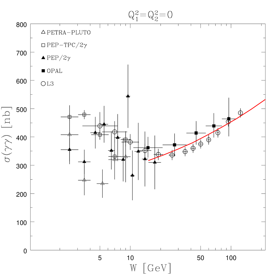
Figure 3: Our calculations for $\sigma(\gamma\gamma)$ and the experimental data.

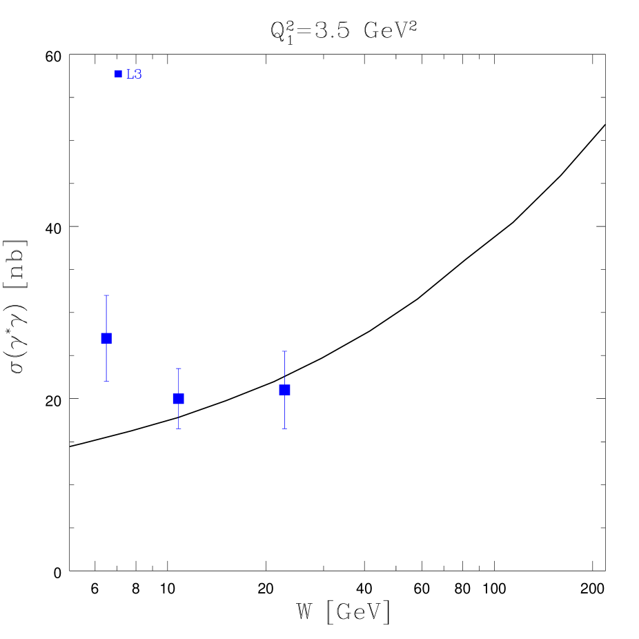
Figure 4: Our calculations for $\sigma(\gamma^{*}\gamma)$ and the experimental data for $Q^{2}_{1}=3.5{\,\mbox{GeV}^{2}}$ and $Q^{2}_{2}=0$.

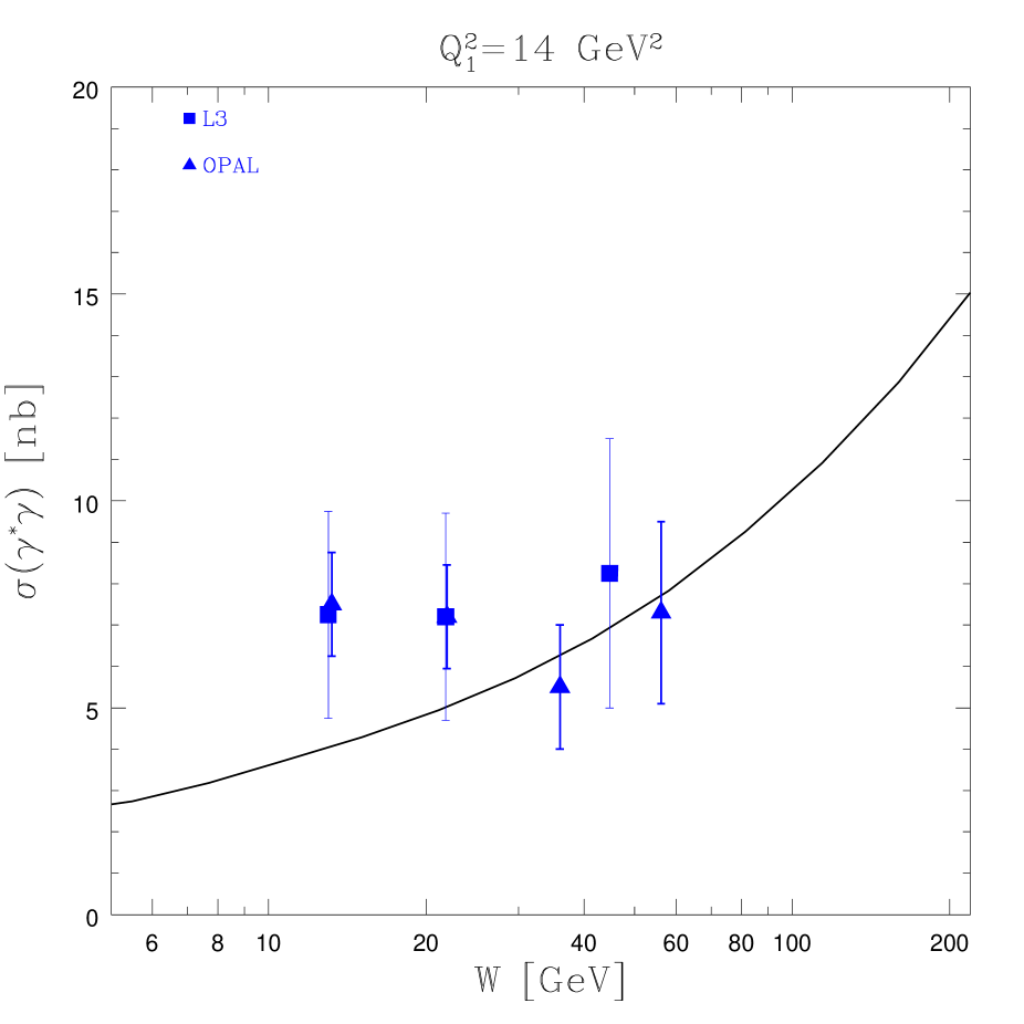
Figure 5: Our calculations for $\sigma(\gamma^{*}\gamma)$ and the experimental data for $Q^{2}_{1}=14{\,\mbox{GeV}^{2}}$ and $Q^{2}_{2}=0$.

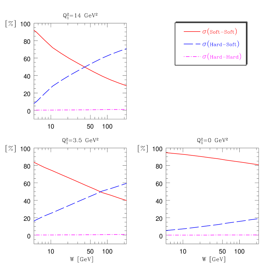
Figure 6: The relative contribution of the three sectors as a percentage from $\sigma(\gamma^{*}\gamma^{*})$ as a function of $W$, for the case of $Q^{2}_{2}=0$.

We initially compare our numerical calculations with the published experimental data [12, 29, 30, 31], in which one photon is always real or semi real (i.e. $Q^{2}_{2}=0$). These are presented in Figs. 3–5, where our calculation and experimental data are plotted as a function of $W$ for fixed $Q^{2}_{1}=0,\,3.5$ and $14{\,\mbox{GeV}^{2}}$. In the region of high energy, we are in good agreement with data at each of the measured virtualities. For real photons, the cross section is dominated by the soft-soft sector, while for the $\gamma^{*}\gamma$ case the hard-soft contribution increases, and at high energies ($\ \raisebox{-1.72218pt}{\hbox to0.0pt{$\sim$\hss}}\raisebox{1.72218pt}{$>$}\ 50{\,\mbox{GeV}^{2}}$) become larger than the soft-soft component [see Fig. 6]. The hard-hard component is small at high energy even for high values $Q^{2}_{1}$. We are unable to reproduce the experimental low energy enhancement which is clearly observed in the data displayed in Figs. 3–5. This is a direct consequence of the threshold enhancement associated with the point like photon component which is not included in our calculations.

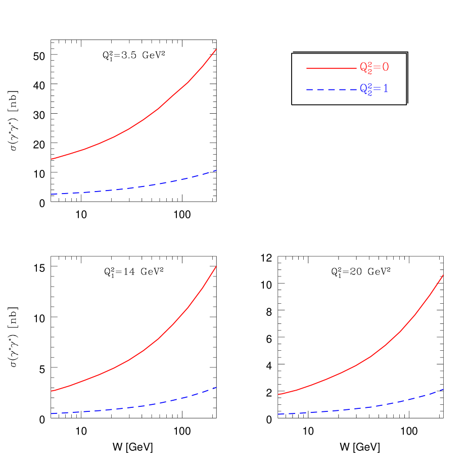
Figure 7: $\sigma(\gamma^{*}\gamma^{*})$ for fixed values of the two photons virtualities.

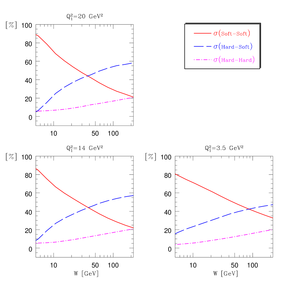
Figure 8: The relative contribution of the three sectors as a percentage from $\sigma(\gamma^{*}\gamma^{*})$ as a function of $W$, for the case of $Q^{2}_{2}=1$.

The total cross section is dramatically reduced when the second photon is virtual. In Fig. 7 we show for comparison the results of the numerical calculation for two processes at fixed $Q^{2}_{1}$ and $Q^{2}_{2}$. The first is the collision of a highly virtual photon ($Q^{2}_{1}=3.5,\,14$ and $20{\,\mbox{GeV}^{2}}$) with a real photon, and the second is the collision of the highly virtual with a semi-hard photon with $Q^{2}_{2}=1{\,\mbox{GeV}^{2}}$. When the second photon is semi-hard, the total cross section is smaller by a factor of 5-7 for $Q^{2}_{1}=3.5{\,\mbox{GeV}^{2}}$ and by a factor of 6-8 for $Q^{2}_{1}=20{\,\mbox{GeV}^{2}}$. The contribution of the hard-hard sector cannot be neglected when $Q^{2}_{2}=1{\,\mbox{GeV}^{2}}$, as can be seen in Fig. 8, where we show the percentage of the three sectors for the semi-hard second photon for fixed values of $Q^{2}_{1}$. This figure is to be compared with Fig. 6.

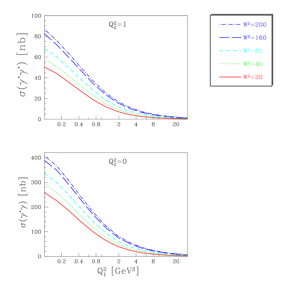
Figure 9: $\sigma(\gamma^{*}\gamma^{*})$ as a function of $Q^{2}_{1}$ for fixed $W$ and two different values of $Q^{2}_{2}$.

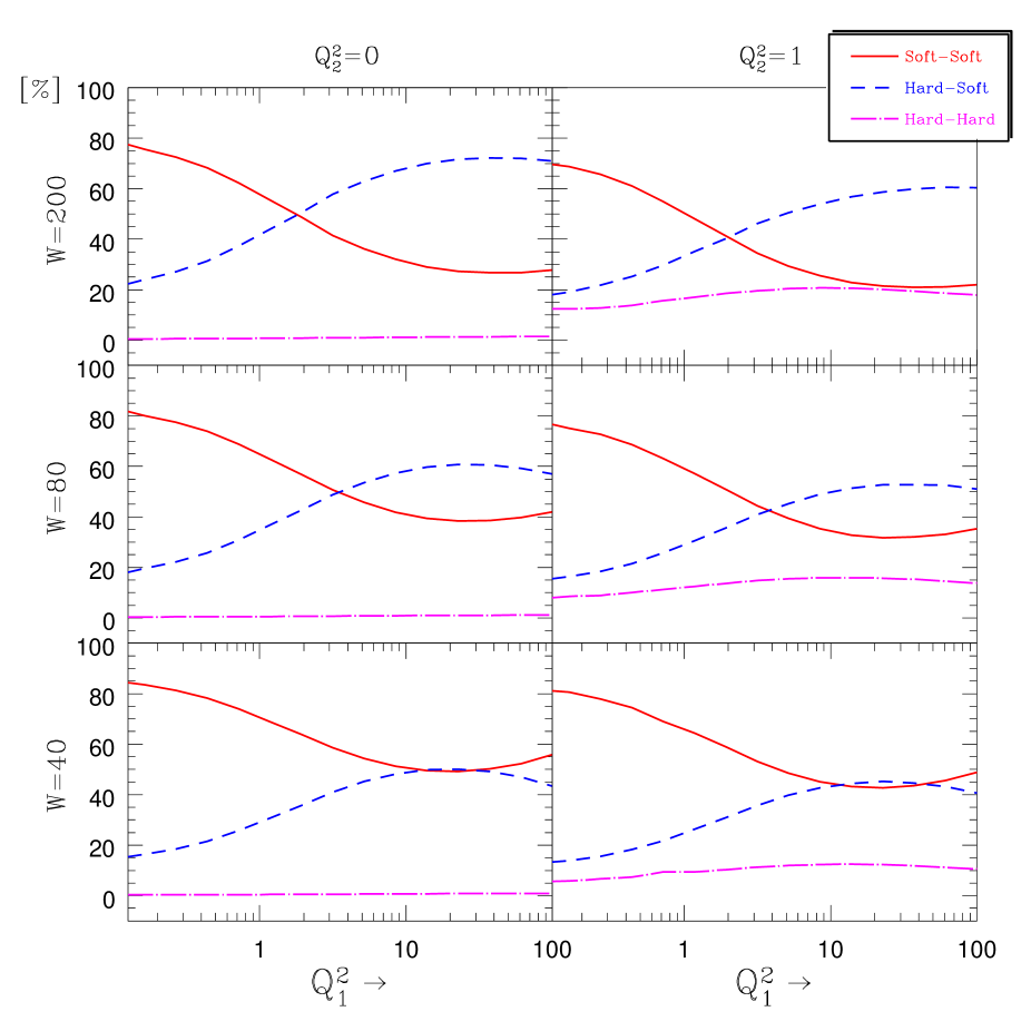
Figure 10: The relative contribution of the soft-soft, hard-soft and hard-hard as a percentage from $\sigma(\gamma^{*}\gamma^{*})$ for fix $W$ and $Q^{2}_{2}$. The three graphs on the left column are for $Q^{2}_{2}=0$ and right column correspond to $Q^{2}_{2}=1$. The values of $W$ are shown on the left hand side of the figure.

It is instructive to study the $Q^{2}$ dependence of our formulae as well. We fixed the value of $W$ and $Q^{2}_{2}$ and calculated the total cross section term by term. It figure Fig. 9 we show the total cross section for two values of $Q^{2}_{2}$ and five values of $W$, and in Fig. 10 we plot the percentage of the three sectors at fix $Q^{2}_{2}$ and $W$. It is worth noting that at high energies and non-zero virtualities the hard-hard sector contribute up to 20% to the total cross section.

As far as the photon’s polarization is concerned, our formalism enables us to define the total cross section as a sum of four expressions: $\sigma^{\mbox{\scriptsize T}}_{\mbox{\scriptsize T}},\,\sigma^{\mbox{\scriptsize T}}_{\mbox{\scriptsize L}},\,\sigma^{\mbox{\scriptsize L}}_{\mbox{\scriptsize T}}$ and $\sigma^{\mbox{\scriptsize L}}_{\mbox{\scriptsize L}}$, where each of these components contain contributions from all the three sectors. For $Q^{2}_{2}=0$, $\sigma^{\mbox{\scriptsize T}}_{\mbox{\scriptsize L}}=\sigma^{\mbox{\scriptsize L}}_{\mbox{\scriptsize L}}=0$ and we are left with only two non-vanishing components which we can use to define the ratio between longitudinal and transverse cross section as $\sigma^{L}/\sigma^{T}=\sigma^{\mbox{\scriptsize L}}_{\mbox{\scriptsize T}}/\sigma^{\mbox{\scriptsize T}}_{\mbox{\scriptsize T}}$. This ratio is shown in Fig. 11, as a function of the energy for constant values of $Q^{2}_{1}$, where the decreasing of the longitudinal component with the energy can be seen. Note that at high energies this ratio approaches the value of $\approx 0.35$ and it does not depend on the value of $Q^{2}_{1}$. However, if the second photon has non-zero virtuality, all of the four components contribute to the total cross section. In Fig. 12 we present the relative contribution of the polarization components as a percentage from $\sigma(\gamma^{*}\gamma^{*})$ both for $Q^{2}_{2}=0$ and $Q^{2}_{2}=1{\,\mbox{GeV}^{2}}$. The contribution to the cross section from the component of two longitudinal photons is less than 5%.

5 Conclusions

In this paper we have presented a detailed calculation of the total cross section for the collision of two virtual photons. Our calculations are based upon a generalization of Gribov’s formula for $\gamma^{*}$p scattering which has been amended for the two photon case. In our approach the parameterization of the two photon interaction is a natural extension of $\gamma$ proton scattering.

We introduce two separation parameters $M^{2}_{0T}$ and $M^{2}_{0L}$ which allows us to stipulate the long and short distance components of the interaction. With the aid of these parameters we are able to separate the two photon cross section into three sectors: soft-soft, hard-soft and hard-hard. This enables us to investigate the interplay between the large and short distance processes, and to evaluate their relative contributions to the total photon-photon cross section. Our calculation of the soft sector is based on the DL parameterization. The hard sector is calculated in pQCD utilizing DGLAP.

The main conclusions of this paper are:

1. For one or two quasi-real photons our model describes the data in the region of high energy (small $x$). Though the $Q^{2}_{1}=Q^{2}_{2}=0$ interaction of two photons is mainly soft, it receives a contribution from what we call the hard-soft sector, which is a signature of short distance processes for one of the photons. On the other hand, even if one photon is highly virtual, the soft-soft sector does not vanish, and therefore npQCD effects also contribute to the hard photon sector.

2. In the case where both photons are off shell, the total cross section is considerably smaller, and the contribution of the hard-hard sector cannot be neglected. This effect occurs already for intermediate distances of the order of $1{\,\mbox{GeV}^{2}}$.

3. Comparing $\sigma(\gamma^{*}\gamma)$ with $\sigma(\gamma^{*}\gamma^{*})$ we observe a somewhat steeper rise of the former as a function of $W$. This stems from the hard-hard sector, which has a moderate energy behaviour, and becomes important only for two off shell photons at high energies.

4. Each of the three sector is a sum of four components for all possible polarizations of the photons. For a realistic situation in which one photon has low virtuality, the cross section is dominated by the transversely polarized photons. Terms in which both photons are longitudinally polarized are small ($<5\%$), while those for mixed polarization are not negligible.

5. The hopes that photon-photon physics in LEP2 and near future $e^{+}e^{-}$ colliders will serve as a clear probe of BFKL dynamics depend on relatively small background from the soft sector and DGLAP hard sector. Not withstanding the expected low statistics of double tagged experiments, we note that these contributions are rather significant at realistic values of the interacting photons virtualities even at high energies.

Acknowledgments: This research was supported in part by the Israel Science Foundation, founded by the Israel Academy of Science and Humanities.

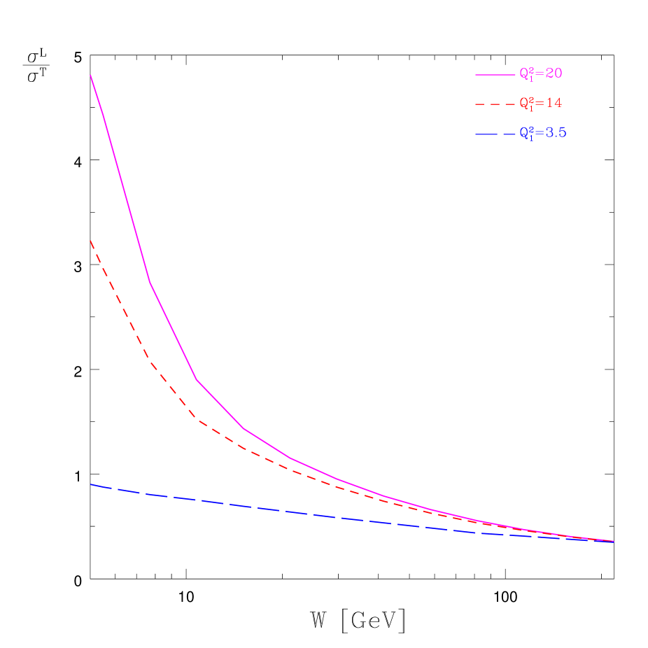
Figure 11: ${\displaystyle\frac{\sigma^{L}}{\sigma^{T}}}$ for the case $Q^{2}_{2}=0$.

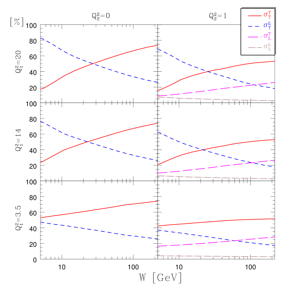
Figure 12: The relative contribution of $\sigma^{\mbox{\scriptsize T}}_{\mbox{\scriptsize T}},\,\sigma^{\mbox{\scriptsize T}}_{\mbox{\scriptsize L}},\,\sigma^{\mbox{\scriptsize L}}_{\mbox{\scriptsize T}}$ and $\sigma^{\mbox{\scriptsize L}}_{\mbox{\scriptsize L}}$ as a percentage from $\sigma(\gamma^{*}\gamma^{*})$ for the case of $Q^{2}_{2}=0$ (left column) and $Q^{2}_{2}=1{\,\mbox{GeV}^{2}}$ (right column). The values of $Q^{2}_{1}$ are shown on the left hand side of the figure.

References

- [1] E. Gotsman, E.M. Levin, U. Maor and E. Naftali, Eur. Phys. J. C10 (1999) 689.
- [2] V.N. Gribov, Sov. Phys. JETP 30 (1970) 709.
- [3] S.J. Brodsky, F. Hautmann and D.E. Soper, Phys. Rev. Lett. 78 (1997) 803.
- [4] M. Boonekamp, A. De Roeck, C. Royon and S. Wallon , Nucl. Phys. B555 (1999) 540.
-
[5]
J. Bartels, A. De Roeck and M. Loewe , Z. Phys. C54 (1992) 635;
J. Bartels, A. De Roeck and H Lotter, Phys. Lett. B389 (1996) 742;
J. Bartels, A. De Roeck, C. Ewerz and H. Lotter, hep-ph/9710500. -
[6]
ECFA/DESY LC Physics Working Group: E. Accomando et al. ,
Phys. Rep. 299 (1998) 1. -
[7]
L.N. Lipatov, Sov. J. Nucl. Phys. 23 (1976) 338;
E.A. Kuraev, L.N. Lipatov and V.S. Fadin, (Sov. Phys. JETP 45 (1977) 199;
I. Balitskii and L.N. Lipatov, Sov. J. Nucl. Phys. 28 (1978) 822. -
[8]
V.N. Gribov and L.N. Lipatov, Sov. J. Nucl. Phys. 15 (1972) 438;
L.N. Lipatov, Yad. Fiz. 20 (1974) 181;
G. Altarelli and G. Parisi, Nucl. Phys. B126 (1977) 298;
Yu.L. Dokshitser, Sov. Phys. JETP 46 (1977) 641. - [9] G.A. Schuler and T. Sjöstrand Z. Phys. C73 (1997) 677.
- [10] M.M. Block, E.M. Gregores, F. Halzen and G. Pancheri, Phys. Rev. D58 (1998) 017503.
-
[11]
M. Rueter, Eur. Phys. J. C7 (1999) 233;
A. Donnachie, H.G. Dosch and M. Rueter Phys. Rev. D59 (1999) 074011;
A. Donnachie, H.G. Dosch and M. Rueter hep-ph/9908413. -
[12]
PLUTO Collaboration, Phys. Lett. B149 (1984) 421;
Z. Phys. C26 (1984) 353;
TPC/ Collaboration, Phys. Rev. D41 (1990) 2667; Phys. Rev. Lett. 54 (1985) 763;
OPAL Collaboration, hep-ex/9906039;
L3 Collaboration, Phys. Lett. B408 (1997) 450. -
[13]
E. Witten, Nucl. Phys. B120 (1977) 189;
C.H. Llewellyn Smith, Phys. Lett. B79 (1978) 83;
W.A. Bardeen and A.J. Buras, Phys. Rev. D20 (1979) 166;
J.H. Field, F. Kapusta and L. Poggioli, Phys. Lett. B181 (1986) 362;
Z. Phys. C36 (1987) 121;
F. Kapusta, Z. Phys. C42 (1989) 225;
W.R. Frazer, Phys. Lett. B194 (1987) 287;
G.A. Schuler and T. Sjöstrand Z. Phys. C68 (1995) 607;
R. Nisius, hep-ex/9912049 and references therein. -
[14]
M. Glück and E. Reya, Phys. Rev. D28 (1983) 2749;
M. Glück, K. Grassie and E. Reya, Phys. Rev. D30 (1984) 1447;
M. Glück, E. Reya and A. Vogt Phys. Rev. D45 (1992) 3986;
M. Glück, E. Reya and A. Vogt Phys. Rev. D46 (1992) 1973. - [15] E. Gotsman, E.M. Levin and U. Maor, Eur. Phys. J. C5 (1998) 303.
-
[16]
P. V. Landshoff and O. Nachtmann, Z. Phys. C35 (1987) 405;
A. Krämer and H.G Dosch, Phys. Lett. B272 (1991) 114;
O. Nachtmann, Annals Phys. 209 (1991) 436;
H.G. Dosch, E. Ferreira and A. Krämer, Phys. Rev. D50 (1994) 1992;
E.R. Berger and O. Nachtmann, Eur. Phys. J. C7 (1999) 459. -
[17]
H.G. Dosch, Phys. Lett. B190 (1987) 555;
H.G. Dosch and Yu.A. Simonov, Phys. Lett. B205 (1988) 339. -
[18]
E.M. Levin and L.L. Frankfurt, JETP Letters 3 (1965) 652;
H.J. Lipkin and F. Scheck, Phys. Rev. Lett. 16 (1966) 71;
J.J.J. Kokkedee, The Quark Model , NY, W.A. Benjamin, 1969. - [19] A. Donnachie and P.V. Landshoff, Phys. Lett. B447 (1998) 408.
- [20] A. Donnachie and S. Soeldner-Rembold, hep-ph/0001035.
-
[21]
B. Badelek and J. Kwiecinski, Z. Phys. C43 (1989) 251; Phys. Lett. B295 (1992) 263;
Phys. Rev. D50 (1994) R4. - [22] A.L. Ayala Filho, M.B. Gay Ducati and E.M. Levin, Eur. Phys. J. C8 (1999) 115.
- [23] E. Gotsman, E.M. Levin, U. Maor and E. Naftali, Nucl. Phys. B539 (1999) 535.
- [24] A. D. Martin, M. G. Ryskin and A. M. Stasto, Eur. Phys. J. C7 (1999) 643.
- [25] E. M. Levin, A. D. Martin, M. G. Ryskin and T. Teubner, Z. Phys. C74 (1997) 671.
-
[26]
A. Donnachie and P.V. Landshoff, Nucl. Phys. B244 (1984) 322;
Nucl. Phys. B267 (1986) 690; Phys. Lett. B296 (1992) 227, Z. Phys. C61 (1994) 139. - [27] M. Glück, E. Reya and A. Vogt, Eur. Phys. J. C5 (1998) 461.
- [28] A.D. Martin, R.G. Roberts, W.J. Stirling, R.S Thorne, hep-ph/9907231.
-
[29]
OPAL Collaboration: F. Wäckerle, Proc. XXVIII int. symp. On
Multiparticle Dynamics,
Frascati, 1997. - [30] L3 Collaboration: M. Acciarri et al. , L3 Note 2400, 1999.
- [31] L3 Collaboration: M. Acciarri et al. , Phys. Lett. B453 (1999) 333.