Contribution of the direct decay $\phi\rightarrow\pi^{+}\pi^{-}\gamma$ to the process $e^{+}e^{-}\to\pi^{+}\pi^{-}\gamma$ at DA$\Phi$NE

Abstract

The potential of DA$\Phi$NE to explore direct radiative decay $\phi\to\pi^{+}\pi^{-}\gamma$ is studied in detail. Predictions of different theoretical models for this decay are compared. We find that it should be possible to discriminate between these models at DA$\Phi$NE in one year, even assuming a relatively low luminosity ${\cal{L}}=10^{31}~{}{\rm cm}^{-2}\,{\rm sec^{-1}}$. The influence of the decay $\phi\to\pi^{+}\pi^{-}\gamma$ on the measurement of total cross section $\sigma(e^{+}e^{-}\to{\rm hadrons})$ by tagging a photon in the reaction $e^{+}e^{-}\to\pi^{+}\pi^{-}\gamma$ is also discussed.

I Introduction

Investigation of CP violation is the most important physical goal of DA$\Phi$NE, a high luminosity $e^{+}e^{-}$ collider which operates on the $\phi(1020)$ resonance. However, thanks to high luminosity, there will be a substantial amount of data which may be used to advance our knowledge on low energy hadron dynamics and even contribute to precision electroweak measurements [1].

Recently it was suggested [2], that the annihilation cross section $\sigma(e^{+}e^{-}\to{\rm hadrons})$ at energies below the mass of the $\phi$ resonance may be studied at DA$\Phi$NE using reaction $e^{+}e^{-}\to{\rm hadrons}+\gamma$. By tagging the photon it is possible to determine the pion form factor at the momentum transfer below the mass of the $\phi$ meson [2]. There are several possibilities to improve further the analysis of [2] and in this paper we consider the contribution of the direct rare decay $\phi\to\pi^{+}\pi^{-}\gamma$ to the reaction $e^{+}e^{-}\to\pi^{+}\pi^{-}\gamma$. Using the terminology of [2], the direct decay contributes to the final state radiation which, for the purpose of the cross section measurement, has to be suppressed by an appropriate choice of cuts on the photon and pion angles and energies. One of the aims of the present paper is to find out how the contribution of the direct decay affects the analysis of Ref.[2].

Besides that, the rare decay $\phi\to\pi^{+}\pi^{-}\gamma$ is an interesting process by itself. As one deals here with the low energy limit of QCD, the first principles calculations are not possible and one has to resort to various models [3, 4, 5, 6, 7, 8]. Since the number of models is flourishing, we think that the experiments should distinguish between them. In principle, that can be achieved by studying the low energy region of the photon spectrum in the reaction $e^{+}e^{-}\to\pi^{+}\pi^{-}\gamma$ [9, 10], but it is not an easy task. The reason is that the relative phases of the direct decay $\phi\to\pi^{+}\pi^{-}\gamma$ and the pure QED processes (initial (ISR) and final (FSR) state radiation) are not predicted by these models. As a consequence, the sign of the interference term appears to be to a large extent arbitrary. If one assumes that the interference is destructive, the branching ratio of the direct decay becomes very small, ${\rm BR}(\phi\to\pi^{+}\pi^{-}\gamma)\approx 4\times 10^{-5}$. Under such circumstances, a detailed study of the decay $\phi\to\pi^{+}\pi^{-}\gamma$ will be rather difficult, requiring high statistics and a careful control over efficiencies in order to discriminate between different models by fitting the photon spectrum.

In this paper we report on the implementation of the direct decay $\phi\to\pi^{+}\pi^{-}\gamma$ into the Monte Carlo event generator for pure QED process $e^{+}e^{-}\to\pi^{+}\pi^{-}\gamma$ described in [2]. Our implementation permits to choose between different models for the decay $\phi\to\pi^{+}\pi^{-}\gamma$. A clear advantage of having a Monte Carlo event generator for these studies is that it allows to keep control over efficiencies and resolution of the detector, fine tuning of the parameters and also provides for the possibility to generate realistic distributions where the reaction $e^{+}e^{-}\rightarrow\pi^{+}\pi^{-}\gamma$ is accompanied by radiation of photons collinear to electrons and positrons [2].

II The matrix element for $\pi^{+}\pi^{-}\gamma$ final state

The matrix element for the direct decay $\phi\to\pi^{+}\pi^{-}\gamma$ is parameterized as:

$${\cal M}_{0}=-ief_{\phi}(Q^{2},Qq){\epsilon_{\phi}}^{\mu}d_{\mu\alpha}{\epsilon}^{\alpha},~{}~{}~{}~{}~{}~{}d_{\mu\alpha}=(Qq)g_{\mu\alpha}-q_{\mu}Q_{\alpha},$$ (1)

where $\epsilon_{\phi}$ and $\epsilon$ are polarizations of the $\phi$ meson and the photon, respectively; $q$ is the momentum of the photon and $Q$ is the momentum of the $\phi$. The function $f_{\phi}(Q^{2},Qq)$ in Eq.(1) is the form factor for the direct decay. Its exact form depends on the chosen model.

Considering production of the $\phi$ meson in $e^{+}e^{-}$ collision with the center of mass energy squared $s=Q^{2}$ and its subsequent decay to $\pi^{+}\pi^{-}\gamma$ final state, we find:

$${\cal M}_{\phi}=\frac{-ie^{3}}{Q^{2}}F_{\phi}(Q^{2},Qq)\bar{v}(p_{2})\gamma_{\mu}u(p_{1})d_{\mu\alpha}{\epsilon}^{\alpha},$$ (2)

where the form factor $F_{\phi}$ is defined as:

$$F_{\phi}=\frac{g_{\phi\gamma}f_{\phi}}{Q^{2}-M_{\phi}^{2}+iM_{\phi}\Gamma_{\phi}}.$$ (3)

The coupling constant $g_{\phi\gamma}$ describes the mixing of the photon and the $\phi$ meson and can be determined from the decay width of the $\phi$ meson into electron positron pair. Using

$$\Gamma(\phi\to e^{+}e^{-})=\frac{4\pi}{3}\frac{g_{\phi\gamma}^{2}\alpha^{2}}{M_{\phi}^{3}}$$ (4)

and $\Gamma(\phi\to e^{+}e^{-})=1.3246\cdot 10^{-6}~{}{\rm GeV}$, $M_{\phi}=1.0194~{}{\rm GeV}$, one obtains $g_{\phi\gamma}=7.929\cdot 10^{-2}~{}{\rm GeV}^{2}$.

Consider now the QED process $e^{-}(p_{1})+e^{+}(p_{2})\to\pi^{+}(\pi_{1})+\pi^{-}(\pi_{2})+\gamma(q)$. The initial state radiation amplitude reads:

$${\cal M}_{isr}=\frac{-ie^{3}F_{\pi}(Q_{1}^{2})}{Q_{1}^{2}}\bar{v}(p_{2})\left[\frac{\gamma_{\mu}(\hat{p}_{1}-\hat{q})\gamma_{\alpha}}{-2p_{1}q}+\frac{\gamma_{\alpha}(-\hat{p}_{2}+\hat{q})\gamma_{\mu}}{-2p_{2}q}\right]u(p_{1})\pi^{\mu}\epsilon^{\alpha},$$ (5)

where $Q_{1}=\pi_{1}+\pi_{2}$ and $\pi=\pi_{1}-\pi_{2}$.

For the amplitude of the final state radiation we obtain:

$${\cal M}_{fsr}=\frac{ie^{3}F_{\pi}(Q^{2})}{Q^{2}}\bar{v}(p_{2})\gamma_{\mu}u(p_{1})$$ (6)

$$\times\left[\frac{2\pi_{2}^{\alpha}+q^{\alpha}}{2\pi_{2}q}(-\pi^{\mu}+q^{\mu})+\frac{(-2\pi_{1}^{\alpha}-q^{\alpha})}{2\pi_{1}q}(-\pi^{\mu}-q^{\mu})-2g^{\alpha\mu}\right]\epsilon_{\alpha}.$$ (7)

Then, the differential cross section for $e^{+}e^{-}\to\pi^{+}\pi^{-}\gamma$ can be written as:

$${\rm d}\sigma_{\rm total}={\rm d}\sigma_{\rm QED}+{\rm d}\sigma_{\phi},$$ (8)

where ${\rm d}\sigma_{\rm QED}$ is the contribution considered in [2]

$${\rm d}\sigma_{\rm QED}\sim|{\cal M}_{isr}+{\cal M}_{fsr}|^{2},$$ (9)

and

$${\rm d}\sigma_{\phi}\sim\left[|{\cal M}_{\phi}|^{2}+2{\rm Re}\left\{{\cal M}_{isr}^{*}{\cal M}_{\phi}\right\}+2{\rm Re}\left\{{\cal M}_{fsr}^{*}{\cal M}_{\phi}\right\}\right]$$ (10)

includes the amplitude of the direct decay. One sees that ${\rm d}\sigma_{\phi}$ contains different interference terms. For this reason one might expect a significant dependence of the $\phi\to\pi^{+}\pi^{-}\gamma$ signal on the relative phases of ${\cal M}_{\phi}$ and ${\cal M}_{isr}+{\cal M}_{fsr}$. We will show below that this is indeed the case. We now describe three different models for the direct decay $\phi\to\pi^{+}\pi^{-}\gamma$ that are implemented in our event generator.

1. “No structure” model [3].

In this case the decay $\phi\to\pi^{+}\pi^{-}\gamma$ occurs through two subsequent transitions $\phi\to f_{0}\gamma\to\pi^{+}\pi^{-}\gamma$. The form factor $f_{\phi}$ in Eq.(1) becomes:

$$f_{\phi}^{no\,str.}=\frac{g_{\phi f_{0}\gamma}g_{f_{0}\pi^{+}\pi^{-}}}{m_{f_{0}}^{2}-Q_{1}^{2}-im_{f_{0}}\Gamma_{f_{0}}}.$$ (11)

The coupling constants in the above equation can be estimated by using the information on the branching ratio ${\rm Br}(\phi\to f_{0}\gamma)$ and on the branching ratio ${\rm Br}(f_{0}\to\pi^{+}\pi^{-})$. One obtains [3]:

$$|g_{\phi f_{0}\gamma}g_{f_{0}\pi^{+}\pi^{-}}|=(144\pm 15)\sqrt{{\rm Br}(\phi\to f_{0}\gamma)}.$$

Needless to say, that the region of applicability of this model is restricted to relatively soft photons, when the $f_{0}$ meson in the intermediate state is not too far off shell. For this reason, when implementing this model into the event generator, we have introduced an additional exponential damping factor which suppresses the emission rate for high energy photons [9]:

$$f_{\phi}^{no\,str.}\rightarrow 1.625\times f_{\phi}^{no\,str.}\exp{\left\{-\frac{(Qq)}{\Delta^{2}}\right\}},$$ (12)

with $\Delta=0.3~{}{\rm GeV}$ [9].

2. $K^{+}K^{-}$ model [5, 4].

In this model one also has a two step transition, similar to “no structure” model. However, the $\phi\to f_{0}\gamma$ decay amplitude is generated dynamically through the loop of charged kaons. The form factor $f_{\phi}$ in Eq.(1) reads:

$$f_{\phi}^{K^{+}K^{-}}=\frac{g_{\phi K^{+}K^{-}}g_{f_{0}\pi^{+}\pi^{-}}g_{f_{0}K^{+}K^{-}}}{2\pi^{2}m^{2}_{K}(m_{f_{0}}^{2}-Q_{1}^{2}-im_{f_{0}}\Gamma_{f_{0}})}I\left(\frac{m_{\phi}^{2}}{m_{K}^{2}},\frac{Q_{1}^{2}}{m_{K}^{2}}\right).$$ (13)

The coupling constants $g_{\phi K^{+}K^{-}},g_{f_{0}\pi^{+}\pi^{-}},g_{f_{0}K^{+}K^{-}}$ can be estimated by using the information on corresponding decay rates [5]:

$$\frac{g^{2}_{\phi K^{+}K^{-}}}{4\pi}=1.66,\,\,\frac{g^{2}_{f_{0}\pi^{+}\pi^{-}}}{4\pi m^{2}_{f_{0}}}=0.105,\,\,\frac{g^{2}_{f_{0}K^{+}K^{-}}}{4\pi}=0.6~{}{\rm GeV}^{2},$$ (14)

and $I(a,b)$ is the function known in the analytic form [5, 4, 11]:

$$I(a,b)=\frac{1}{2(a-b)}-\frac{2}{(a-b)^{2}}\left[f(b^{-1})-f(a^{-1})\right]+\frac{a}{(a-b)^{2}}\left[g(b^{-1})-g(a^{-1})\right].$$ (15)

The functions $f(x)$ and $g(x)$ are given by:

$$\begin{array}[]{l}f(x)=\left\{\vspace{-.5cm}\begin{array}[]{cl}-\arcsin^{2}\frac{1}{2\sqrt{x}}~{}~{}~{}~{}~{}~{}~{}~{}~{}~{}~{}~{}~{}~{}~{}~{}~{}x>\frac{1}{4},\\ \frac{1}{4}[\ln\frac{\eta_{+}}{\eta_{-}}-i\pi]^{2}~{}~{}~{}~{}~{}~{}~{}~{}~{}~{}~{}~{}~{}~{}~{}~{}x<\frac{1}{4},\end{array}\right.\\[19.37494pt] g(x)=\left\{\vspace{-.5cm}\begin{array}[]{c l}\sqrt{4x-1}\arcsin\frac{1}{2\sqrt{x}}~{}~{}~{}~{}~{}~{}~{}~{}~{}~{}x>\frac{1}{4},\\ \frac{1}{2}\sqrt{1-4x}[\ln\frac{\eta_{+}}{\eta_{-}}-i\pi]~{}~{}~{}~{}~{}~{}~{}x<\frac{1}{4},\end{array}\right.\end{array}$$ (16)

with $\eta_{\pm}=(1\pm\sqrt{1-4x})/(2x)$.

3. Chiral Unitary Approach ($U\chi PT$) [8, 11].

In this case the decay $\phi\to\pi^{+}\pi^{-}\gamma$ occurs through a loop of charged kaons that subsequently annihilate into $\pi^{+}\pi^{-}\gamma$. The $f_{0}$ resonance is generated dynamically by unitarizing the one-loop amplitude. Using notations of Ref.[8], the form factor $f_{\phi}$ in Eq.(1) reads:

$$f_{\phi}^{U\chi PT}=t_{\rm ch}\left\{\frac{G_{V}M_{\phi}}{f_{\pi}^{2}2\sqrt{2}\pi^{2}m_{K}^{2}}I\left(\frac{m_{\phi}^{2}}{m_{K}^{2}},\frac{Q_{1}^{2}}{m_{K}^{2}}\right)+\frac{\sqrt{2}}{M_{\phi}f_{\pi}^{2}}\left(\frac{F_{V}}{2}-G_{V}\right)G_{K^{+}K^{-}}\right\},$$ (17)

where the coupling $G_{V}$ and $F_{V}$ are related to the decays $\phi\to K^{+}K^{-}$ and $\phi\to e^{+}e^{-}$, respectively, $f_{\pi}$ is the pion decay constant and $I(a,b)$ is the function given in Eq.(15). $G_{K^{+}K^{-}}$ is defined by the integral:

$$G_{K^{+}K^{-}}=\frac{1}{2\pi^{2}}\int_{0}^{q_{\rm max}}\frac{q^{2}dq}{\sqrt{q^{2}+m_{K}^{2}}\left(Q_{1}^{2}-4(q^{2}+m_{K}^{2})+i\epsilon\right)}.$$ (18)

In Eq.(17) $t_{\rm ch}$ is the strong scattering amplitude

$$t_{\rm ch}=\frac{1}{\sqrt{3}}t_{K\bar{K},\pi\pi}^{I=0}.$$ (19)

The scattering amplitude $t_{K\bar{K},\pi\pi}^{I=0}$ is determined by using chiral perturbation theory (see Ref.[7]). We have used the following values for the above constants: $G_{V}=0.055~{}{\rm GeV}$, $F_{V}=0.165~{}{\rm GeV}$, $f_{\pi}=0.093~{}{\rm GeV}$, $q_{\rm max}=0.9~{}{\rm GeV}$.

In Fig.1 we present a comparison of the photon spectrum obtained using the event generator and retaining only the term $|{\cal M}_{\phi}|^{2}$ in the cross section (cf. Eq.(10)), with the analytic expressions from Refs.[3, 5, 8]. One sees a good agreement between the Monte Carlo simulation and the analytic results. Note also, that different models predict different shapes of the photon spectrum.

III Studying the direct decay $\phi\to\pi^{+}\pi^{-}\gamma$ at DA$\Phi$NE

We now address the question of whether precision studies of the direct decay $\phi\to\pi^{+}\pi^{-}\gamma$ are possible at DA$\Phi$NE. While writing the general formula for the process $e^{+}e^{-}\to\pi^{+}\pi^{-}\gamma$, we have pointed out that the observable signal of $\phi\to\pi^{+}\pi^{-}\gamma$ might strongly depend on the interference with the FSR. The $f_{0}$ signal may be enhanced if the sign between $|{\cal M}_{\phi}|^{2}$ and $2{\rm Re}\left\{{\cal M}_{fsr}^{*}{\cal M}_{\phi}\right\}$ is the same (constructive interference) or may be reduced in the opposite case (destructive interference).

In Fig.2 we present the spectrum of photons in the reaction $e^{+}e^{-}\to\pi^{+}\pi^{-}\gamma$ in the situation when the invariant mass of two pions is close to the mass of the $f_{0}$ meson. We consider both constructive and destructive interference and generate events with and without collinear radiation, but initial and final state radiation is always kept. One sees from Fig.2 that the collinear radiation results in the reduction of the signal. However, if the tagged photon is emitted at a relatively large angle, the effect of collinear radiation can be partially removed by combining the information on the position of the neutral cluster in the calorimeter with the directions of the charged pions determined with the drift chamber. In this case the kinematics of the reaction becomes over-constrained and it is possible to restore the “actual” center of mass energy for any given event. This will require a dedicated analysis, however.

Fig.3 shows the signal-to-background ratio

$$S/B=\frac{{\rm d}\sigma_{\rm total}}{{\rm d}\sigma_{\rm QED}}$$ (20)

for different models. As expected, the sign of the interference affects not only the magnitude of the decay $\phi\to\pi^{+}\pi^{-}\gamma$, but also the shape of the distribution. The models where the structure of the $f_{0}$ meson is assumed show a broader signal for the constructive interference than in the opposite case. In addition, the “no structure” model does not show a clear peak in the case of destructive interference and the $U\chi PT$ model in the case of constructive interference.

The number of events required to separate the signal from the background can be obtained by estimating the necessary number of events in the energy region around the $f_{0}$ peak. We require the statistical error to be smaller than $10$% of the signal itself. Hence,

$$\delta N\leq\frac{\Delta N}{10},$$ (21)

where $\Delta N$ is the number of events due to direct decay of the $\phi$ meson:

$$\Delta N=N_{\rm total}-N_{\rm QED}.$$ (22)

If we introduce a parameter $\xi$ such that

$$N_{\rm total}=(1+\xi)N_{\rm QED},$$ (23)

Eq.(21) takes the form:

$$\delta N\leq\frac{\xi N_{QED}}{10}.$$ (24)

The value of $\xi$ can be estimated from the $S/B$ ratio shown in Fig.3. Using the standard formula for statistical fluctuation, $\delta N=\sqrt{N_{\rm total}}$, we estimate the number of events required to separate the contribution of $\phi\to\pi^{+}\pi^{-}\gamma$ from the QED background:

$$N_{\rm QED}\geq(1+\xi)\left(\frac{10}{\xi}\right)^{2},~{}~{}~{}~{}{\cal{L}}\geq\frac{N_{\rm QED}}{\epsilon\sigma_{\rm QED}}.$$ (25)

Here $\epsilon$ is the overall detector efficiency for $\pi^{+}\pi^{-}\gamma$ events and ${\cal L}$ is the required integrated luminosity.

The results are summarized in Table I. We use $\epsilon=0.5$ and $\sigma_{\rm QED}=2.1~{}{\rm nb}$ with the cuts $|\cos{\theta_{\gamma}}|<0.9$, $|\cos{\theta_{\pi^{\pm}}}|<0.9$, $|\cos{\theta_{\pi\gamma}}|<0.9$ ( without collinear radiation). When the collinear radiation is included, $\sigma_{\rm QED}$ is reduced to approximately $2~{}{\rm nb}$.

without collinear rad.
Models	Construct. interf.			Destruct. interf.
	$\xi$	$\#{\rm events}$	${\cal{L}}({\rm pb}^{-1})$	$\xi$	$\#{\rm events}$	${\cal{L}}({\rm pb}^{-1})$
No struct	0.35	1100	1	0.01	$10^{6}$	$\sim 2\times 10^{3}$
		$20~{}{\rm MeV}<E_{\gamma}<100~{}{\rm MeV}$			$20~{}{\rm MeV}<E_{\gamma}<100~{}{\rm MeV}$
$K^{+}K^{-}$	0.22	$\sim 2100$	$2$	0.07	$22\times 10^{3}$	40
		$20~{}{\rm MeV}<E_{\gamma}<100~{}{\rm MeV}$			$20~{}{\rm MeV}<E_{\gamma}<50~{}{\rm MeV}$
$U\chi PT$	0.1	$11\times 10^{4}$	$\sim 11$	0.15	5100	9
		$20~{}{\rm MeV}<E_{\gamma}<100~{}{\rm MeV}$			$20~{}{\rm MeV}<E_{\gamma}<50~{}{\rm MeV}$
with collinear rad.
Models	Construct. interf.			Destruct. interf.
	$\xi$	$\#{\rm events}$	${\cal{L}}({\rm pb}^{-1})$	$\xi$	$\#{\rm events}$	${\cal{L}}({\rm pb}^{-1})$
No struct	0.25	$\sim 2000$	$\sim 2$	0.01	$10^{6}$	$\sim 2\times 10^{3}$
		$20~{}{\rm MeV}<E_{\gamma}<100~{}{\rm MeV}$			$20~{}{\rm MeV}<E_{\gamma}<100~{}{\rm MeV}$
$K^{+}K^{-}$	0.16	$\sim 4500$	$\sim 4$	0.04	$65\times 10^{3}$	118
		$20~{}{\rm MeV}<E_{\gamma}<100~{}{\rm MeV}$			$20~{}{\rm MeV}<E_{\gamma}<50~{}{\rm MeV}$
$U\chi PT$	0.08	$\sim 17000$	16	0.1	$11\times 10^{3}$	20
		$20~{}{\rm MeV}<E_{\gamma}<100~{}{\rm MeV}$			$20~{}{\rm MeV}<E_{\gamma}<50~{}{\rm MeV}$

TABLE I.: The number of events and the integrated luminosity required to observe the direct decay $\phi\to\pi^{+}\pi^{-}\gamma$.

In a similar way we make a rough estimate of the number of events and the luminosity required to discriminate between different models for the direct decay. We obtain:

$$N_{\rm QED}\geq\left(\frac{10}{\xi_{12}}\right)^{2},$$ (26)

with

$$\xi_{12}=\xi_{1}-\xi_{2},$$ (27)

and $\xi_{1,2}$ are the $\xi$-parameters for two models under consideration. In Table II we summarize the results. One can see that the required number of events can be accumulated at DA$\Phi$NE in less than one year assuming the luminosity ${\cal{L}}=10^{31}~{}{\rm cm}^{-2}\,{\rm sec^{-1}}$. The required luminosity is, however, only indicative.

	without coll. rad.			with coll. rad.
Models	Construct. interf.
	$\xi_{12}$	$\#{\rm events}$	${\cal{L}}({\rm pb}^{-1})$	$\xi_{12}$	$\#{\rm events}$	${\cal{L}}({\rm pb}^{-1})$
No struct vs. $K^{+}K^{-}$	0.13	$6\times 10^{3}$	$\sim 5$	0.09	$\sim 11\times 10^{3}$	$\sim 11$
	Destruct. interf.
	$\xi_{12}$	$\#{\rm events}$	${\cal{L}}({\rm pb}^{-1})$	$\xi_{12}$	$\#{\rm events}$	${\cal{L}}({\rm pb}^{-1})$
$K^{+}K^{-}$ vs. $U\chi PT$	0.08	$16\times 10^{3}$	29	0.06	$26\times 10^{3}$	47

TABLE II.: The number of events and the integrated luminosity required to distinguish between two different models for the rare decay $\phi\to\pi^{+}\pi^{-}\gamma$.

IV Direct decay of the $\phi$ meson and the measurement of the electron positron annihilation cross section at DA$\Phi$NE

It was suggested in Ref.[2] that the measurement of $\sigma(e^{+}e^{-}\to{\rm hadrons})$ at DA$\Phi$NE for different values of the center of mass energy can be performed by analyzing events with additional hard photon emitted at a relatively large angle ($\theta_{\gamma}>7^{o}$). The difficulties of this approach are related to the obvious fact that the hard photon can be emitted from both initial and final state of the process. If the ISR takes place, the total energy of the collision is reduced and such events can be used to measure $\sigma(e^{+}e^{-}\to{\rm hadrons})$ at different energies. In contrast to that, the photons caused by the FSR represent a background that must be suppressed by applying suitable cuts. Since, to be competitive[1, 2], the measurement of $\sigma(e^{+}e^{-}\to{\rm hadrons})$ for $\sqrt{s}<1~{}{\rm GeV}$ has to be performed at the one percent level, the practical realization of this idea is a non-trivial experimental task. In Ref.[2] only the QED process was studied. Here we would like to add the direct decay $\phi\to\pi^{+}\pi^{-}\gamma$ which also contributes to the FSR and therefore increases the background. In Fig.4 we show the values of $({\rm d}\sigma_{{\rm total}}/{\rm d}E_{\gamma})/({\rm d}\sigma_{\rm ISR}/{\rm d}E_{\gamma})$ with and without the contribution of the direct decay. The “pure QED” case was studied in Ref.[2]. The photon energies $20~{}{\rm MeV}<E_{\gamma}<100~{}{\rm MeV}$ are considered, which corresponds to $0.836~{}{\rm GeV}^{2}<Q_{\pi^{+}\pi^{-}}^{2}<0.996~{}{\rm GeV}^{2}$. These invariant masses of two pions include the contribution of the $f_{0}$ resonance and for this reason the largest contribution of the direct decay is expected in this region. The cuts reduce the FSR considerably; nevertheless, its contribution close to $f_{0}$ peak is significant.

As discussed in [2], even “pure QED” theoretical predictions for the FSR are, strictly speaking, model dependent. It is therefore important to get a handle on it experimentally. In Ref. [2] it was suggested to use the forward-backward asymmetry of the produced pions to control the FSR. The direct decay $\phi\to\pi^{+}\pi^{-}\gamma$ changes the forward-backward asymmetry in the expected manner. Since the contribution of the direct decay is significant only if the invariant mass of the two pions is close to the mass of the $f_{0}$ meson, the forward-backward asymmetry integrated over large range of $Q_{\pi^{+}\pi^{-}}^{2}$ is not affected by the direct decay. Hence it can be used to control the models for QED-like final state radiation. On the other hand, by applying the cut $0.836~{}{\rm GeV}^{2}<Q_{\pi^{+}\pi^{-}}^{2}<0.996~{}{\rm GeV}^{2}$, we significantly enhance the contribution of the direct decay to forward-backward asymmetry. This is shown in Fig.5 where predictions of $K^{+}K^{-}$ model are displayed for both constructive and destructive interference.

V Conclusions

We have discussed the contribution of the direct decay $\phi\to\pi^{+}\pi^{-}\gamma$ to the process $e^{+}e^{-}\to\pi^{+}\pi^{-}\gamma$ at DA$\Phi$NE energies. To facilitate this study, three different models for the direct decay $\phi\to\pi^{+}\pi^{-}\gamma$ have been implemented into the Monte Carlo event generator described in Ref.[2].

The importance of this decay is twofold. First, it gives the information about the nature of the $f_{0}(980)$ meson. Second, it provides an additional background to the measurement of $\sigma(e^{+}e^{-}\to\pi^{+}\pi^{-})$ at different values of the center of mass energy by tagging the hard photon in the reaction $e^{+}e^{-}\to\pi^{+}\pi^{-}\gamma$.

We have shown that DA$\Phi$NE has a very good potential to study the nature of $f_{0}$ resonance. Even with moderate luminosity ${\cal{L}}=10^{31}~{}{\rm cm}^{-2}\,{\rm sec^{-1}}$, it is possible to discriminate between different models for the decay $\phi\to\pi^{+}\pi^{-}\gamma$ in a relatively short time.

As for the measurement of the hadronic cross section $\sigma(e^{+}e^{-}\to{\rm hadrons})$ at $\sqrt{s}<1~{}{\rm GeV}$ using the process $e^{+}e^{-}\to\pi^{+}\pi^{-}\gamma$, we have found that the direct decay $\phi\to\pi^{+}\pi^{-}\gamma$ increases the final state radiation by several percent in the region of pion invariant masses $0.836~{}{\rm GeV}^{2}<Q_{\pi^{+}\pi^{-}}^{2}<0.996~{}{\rm GeV}^{2}$, but quickly dies out beyond this region.

Finally, we note that it will also be possible to perform a detailed study of the decay $\phi\to\pi^{o}\pi^{o}\gamma$ at DA$\Phi$NE . We believe that it will be quite useful to combine these independent measurements in order to check the theoretical understanding of the $f_{0}$ meson.

VI Acknowledgments

We are grateful to J.H. Kühn, W. Kluge, G. Pancheri, M. Greco, A. Denig and G. Cataldi for useful discussions and E. Marco for providing us with his code. We also thank M.Pennington for organizing a pleasant EuroDA$\Phi$NE meeting in Durham where part of this work was done.

This work is supported by the EU Network EURODAPHNE, contract FMRX-CT98-0169, by BMBF under the contracts BMBF-06KA860 and BMBF-057KA92P, by the United States Department of Energy, contract DE-AC03-76SF00515, by Graduiertenkolleg “Elementarteilchenphysik an Beschleunigern” at the University of Karlsruhe and by the DFG Forschergruppe “Quantenfeldtheorie, Computeralgebra und Monte-Carlo-Simulation”

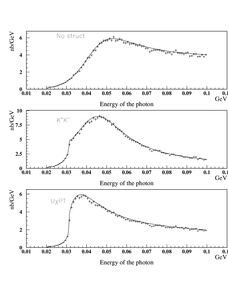
FIG. 1.: The energy spectrum of photons produced in the direct decay $\phi\to\pi^{+}\pi^{-}\gamma$ without initial and final state radiation. The results of the Monte Carlo simulation are compared with the results of analytical calculations (solid curves) for different models [3, 5, 8]. We use $m_{f_{0}}=0.976~{}{\rm GeV}$, $\Gamma_{f_{0}}=34~{}{\rm MeV}$. For the “no structure” model the branching ratio ${\rm Br}(\phi\to f_{0}\gamma)=10^{-4}$ has been used as an input (this branching ratio is of the same order of magnitude as is predicted by the other two models). For the purpose of comparison, no exponential damping has been applied to the “no structure” model and the events were generated without collinear radiation. We have applied the following cuts on the polar angle and the energy of the photons: $10^{o}<\theta_{\gamma}<170^{o}$, $20~{}{\rm MeV}~{}<E_{\gamma}<100~{}{\rm MeV}$.

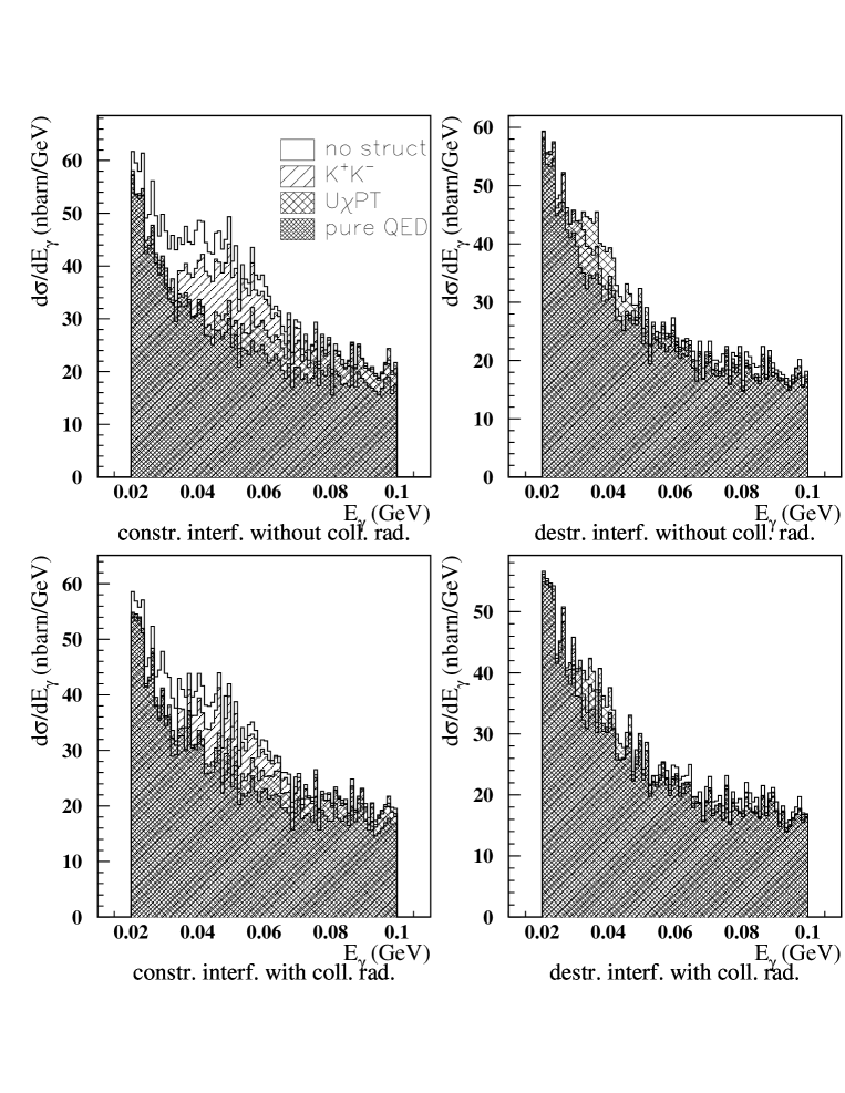
FIG. 2.: The spectrum of photons in the reaction $e^{+}e^{-}\to\pi^{+}\pi^{-}\gamma$. The following cuts were applied: $|\cos{\theta_{\gamma}}|<0.9$, $|\cos{\theta_{\pi^{\pm}}}|<0.9$, $|\cos{\theta_{\pi\gamma}}|<0.9$, where $\theta_{\gamma}$ and $\theta_{\pi}$ are the polar angles of photon and pions, respectively, and $\theta_{\pi\gamma}$ is the angle between the photon and the $\pi^{+}$ momenta in the center of mass frame of the two pions. The exponential damping was applied to the ‘no structure‘” model and the branching ratio ${\rm Br}(\phi\to f_{0}\gamma)=2.5\times 10^{-4}$ has been chosen. Different models are distinguished by different hatching. “Pure QED” means that only the contribution due to ${\rm d}\sigma_{\rm QED}$ is considered.

FIG. 3.: The signal-to-background ratio $({\rm d}\sigma_{\rm total}/{\rm d}E_{\gamma})/({\rm d}\sigma_{\rm QED}/{\rm d}E_{\gamma})$ as a function of photon energy. The cuts are $|\cos{\theta_{\gamma}}|<0.9$, $|\cos{\theta_{\pi^{\pm}}}|<0.9$, $|\cos{\theta_{\pi\gamma}}|<0.9$. See text for more details.

FIG. 4.: Ratio $({\rm d}\sigma_{{\rm total}}/{\rm d}E_{\gamma})/({\rm d}\sigma_{\rm ISR}/{\rm d}E_{\gamma})$ as a function of the energy of the photon. The cuts are $7^{o}<\theta_{\gamma}<20^{o}$, $30^{o}<\theta_{\pi}<150^{o}$, and the invariant mass of detected particles in the final state $Q^{2}_{\pi^{+}\pi^{-}\gamma}>0.9~{}{\rm GeV}^{2}$. “Pure QED” ratio is defined as $({\rm d}\sigma_{\rm ISR+FSR}/{\rm d}E_{\gamma})/({\rm d}\sigma_{\rm ISR}/{\rm d}E_{\gamma}.)$ Different pictures correspond to different models for the $f_{0}$ resonance. The cases of constructive and destructive interference are considered. See text for more details.

FIG. 5.: $\pi^{+}$ angular distribution. The photon angle is $60^{o}<\theta_{\gamma}<120^{o}$. The invariant mass of the two pions is $0.836~{}{\rm GeV}^{2}<Q_{\pi^{+}\pi^{-}}^{2}<0.996~{}{\rm GeV}^{2}$.

REFERENCES

• [1] S.Β Eidelman, F.Β Jegerlehner, Z. fΓΌr. Physik C67, 585 (1995).
• [2] S.Β Binner, J.H.Β KΓΌhn, K.Β Melnikov, Phys. Lett. B459, 279 (1999).
• [3] A.Β Bramon, G.Β Colangelo and M.Greco, Phys. Lett. B287, 263 (1992).
• [4] F.E.Β Close, N.Β Isgur, S.Β Kumano, Nucl. Phys. B389, 513 (1993).
• [5] J.L.Β Lucio M., M.Β Napsuciale, Phys. Lett. B331, 418 (1994).
• [6] N.N.Β Achasov, V.V.Β Gubin, and E.P.Β Solodov, Phys. Rev. D55, 2672 (1997).
• [7] J.A.Β Oller, E.Β Oset, Nucl. Phys. A620, 438 (1997).
• [8] E.Β Marco, S.Β Hirenzaki, E.Β Oset, H.Β Toki, hep-ph/9903217.
• [9] P.J.Β Franzini, W.Β Kim and J.L.Β Franzini, Phys. Lett. B287, 259 (1992).
• [10] R.R.Β Akhmetshin et al., hep-ex/9907005.
• [11] J.A.Β Oller, Phys. Lett. B426, 7 (1998).
Refer to caption