CERN-TH/99-356

TTP99-55

hep-ph/0001062

December 1999

Quarkonium momentum distributions
in photoproduction and $B$ decay
M. Beneke   and    G.A. Schuler Theory Division, CERN, CH-1211 Geneva 23, Switzerland
and
S. Wolf Institut für Theoretische Teilchenphysik, Universität Karlsruhe,
D-76128 Karlsruhe, Germany

According to our present understanding many $J/\psi$ production processes proceed through a coloured $c\bar{c}$ state followed by the emission of soft particles in the quarkonium rest frame. The kinematic effect of soft particle emission is usually a higher-order effect in the non-relativistic expansion, but becomes important near the kinematic endpoint of quarkonium energy (momentum) distributions. In an intermediate region a systematic resummation of the non-relativistic expansion leads to the introduction of so-called ‘shape functions’. In this paper we provide an implementation of the kinematic effect of soft gluon emission which is consistent with the non-relativistic shape function formalism in the region where it is applicable and which models the extreme endpoint region. We then apply the model to photoproduction of $J/\psi$ and $J/\psi$ production in $B$ meson decay. A satisfactory description of $B$ decay data is obtained. For inelastic charmonium photoproduction we conclude that a sensible comparison of theory with data requires a transverse momentum cut larger than the currently used 1 GeV.

PACS Nos.: 13.85.Ni, 14.40.Gx

I Introduction

Inclusive charmonium production processes can be expressed in a factorized form, combining a short-distance expansion with the use of a non-relativistic QCD Lagrangian (NRQCD) [1]. The short-distance expansion works best for total production cross sections, provided the expansion parameter $v^{2}$ (of order of the typical velocity squared of the quarks in the bound state) is small enough. It follows that contrary to prior belief many charmonium production processes such as production in hadron-hadron collisions at large transverse momentum [2] and at fixed target [3], and in $B$ meson decay [4, 5, 6, 7], are actually dominated by production of a coloured $c\bar{c}$ state, followed by a long-distance transition to charmonium and light hadrons [8].

The theoretical prediction of charmonium energy distributions is more delicate. A long-standing problem for the NRQCD factorization approach concerns the $z$-distribution in inelastic $J/\psi$ photoproduction, where $z=E_{J/\psi}/E_{\gamma}$ is the quarkonium energy fraction in the proton rest frame. The colour octet contributions to this quantity grow rapidly near $z=1$ [9, 6], in conflict with observation [10], unless the NRQCD matrix elements that normalize the colour octet contribution are made rather small.

One of the physical origins of this discrepancy is as follows: the fragmentation of the coloured $c\bar{c}$ state into $J/\psi$ occurs via the emission of gluons with small momentum fractions of order $v^{2}$. Because the momentum of these gluons is small compared to the momenta involved in the hard subprocess that creates the $c\bar{c}$ state, it is neglected in leading order in the short-distance expansion (in $v^{2}$); the fragmentation into $J/\psi$ is described by a single number (the ‘NRQCD matrix element’). This is adequate for total production cross sections, but it is not for distributions in the kinematic region, where the charmonium carries nearly maximal energy. In this region, the $J/\psi$ energy distribution is evidently sensitive to the energy distribution of the soft emitted gluons. In particular, we expect that the $J/\psi$ energy distribution should fall to zero, rather than grow, near the point of maximal energy, if the $J/\psi$ is produced via a colour octet state, since the emission of gluons with momentum much smaller than their typical one is rather unlikely.

The inadequacy of a leading-order treatment of the short-distance expansion, and the necessity to account for the kinematics of soft gluon emission, is even more evident for $J/\psi$ production in $B$ meson decay. The leading order partonic short-distance process $b\to(c\bar{c})q$ results in $c\bar{c}$ pairs with fixed (maximal) energy, in stark contrast to the broad energy distribution observed [16]. The broad energy distribution of multi-body final states has to be attributed to soft gluon emission and to the Fermi motion of the $b$ quark in the $B$ meson.

Technically speaking, the velocity expansion of the short-distance process breaks down near the kinematic endpoint of maximal charmonium energy [17, 18], because higher-order terms in the small parameter $v^{2}$ are compensated by inverse powers of small kinematic invariants. Such a breakdown of the short-distance expansion is not specific to quarkonium production in the NRQCD approach, but occurs quite generally for inclusive processes, for example in deep-inelastic scattering as Bjorken $x\to 1$ or in semi-leptonic or radiative $B$ decays [19]. When the quarkonium carries a fraction $(1-\epsilon)$ of its maximal energy, where $\epsilon$ is small, the inclusiveness of the process is restricted by the small phase-space left for the emission of further particles. The process is then also sensitive to the fact that the physical phase space is limited by hadron kinematics, while the calculation of short-distance coefficients is carried out in terms of partons. The short-distance expansion reacts to this non-inclusiveness by exhibiting terms of order $(v^{2}/\epsilon)^{k}$. In some cases one can sum the leading terms in $v^{2}/\epsilon$ to all orders and express the quarkonium production cross section as a convolution of a non-perturbative ‘shape function’ with a partonic cross section. The shape function leads to a smearing of the energy spectrum. The shape function formalism is analogous to a leading twist approximation, and is appropriate for $\epsilon\sim v^{2}$. In this intermediate region the framework of the NRQCD factorization approach is still valid, reorganized by a partial resummation of the velocity expansion. However, in the extreme endpoint region, $\epsilon\ll v^{2}$, the twist expansion also breaks down.

The leading twist expressions for several energy distributions have been derived in [18]. But since the shape function is non-perturbative and essentially unknown, no quantitative analysis has been performed. It is the aim of this paper to explore the kinematic effect of soft gluons in the fragmentation of a coloured $c\bar{c}$ pair quantitatively. In particular, we will be interested in the question whether folding the short-distance cross section with a shape function can indeed account for the observed $z$-distribution in $J/\psi$ photoproduction. The emission of soft gluons with energy of order $m_{c}v^{2}$ in the quarkonium rest frame cannot be computed perturbatively and we have to model it. Our ansatz for the soft gluon radiation function will be guided by simplicity. The important feature of the model is that it incorporates the kinematics of soft gluon radiation together with reasonable assumptions on the typical energy scales involved. The ansatz bears some similarities with Fermi motion smearing [20] and, in particular, the ACCMM model [21] for semileptonic $B$ decays. Since the precise form of the energy distribution near the endpoint depends on the ansatz for the shape function, our results do not constitute theoretical predictions. However, as we shall see, a satisfactory description of $B$ decay data can indeed be obtained with a reasonable ansatz for the shape function. A further cross check is provided by applying the same shape function to the $J/\psi$ energy distribution in photoproduction. This however, turns out to be more problematic.

The paper is divided as follows: Sect. 2 is ‘theoretical’. We define the model and derive the equation that describes the convolution of the short-distance process with the shape function for a general production process. We also show that the model is equivalent to a specific form of the NRQCD shape function in the region where a leading twist approximation is valid. To illustrate the formalism, we consider the limit $m_{c}v^{2}\gg\Lambda_{\rm QCD}$, in which charmonium is a Coulomb bound state. We rederive NRQCD factorization for this specific case and compute the shape function in this limit.

The ansatz for the non-perturbative shape function depends on a few model parameters. In Sect. 3 we apply the model to the $J/\psi$ momentum distribution in $B\to J/\psi+X$ and tune the parameters of the model to the observed momentum distribution. In Sect. 4 the more complicated (and more interesting) case of inelastic photoproduction is considered.

II Shape function model

In this section we derive the general expression for the smeared quarkonium energy distributions on which the applications to $B$ decay and photoproduction will be based. To motivate our approach and to make more explicit contact with the formalism of [1, 18], we begin by considering the production amplitude for quarkonium in the Coulomb limit, and with emission of a single soft gluon, before generalizing the expressions to the case of interest. In the last subsection we return to the Coulomb limit and compute the shape function in this limit. This provides us with an idea of the form of the shape function in a controlled, although unrealistic limit.

A Factorization and the shape function in the Coulomb limit

Inclusive charmonium production proceeds in two stages [1]: first a pair of nearly on-shell and co-moving charm quarks is created in a hard process in which typical momenta are of order $2m_{c}$ (or larger, if there is another hard scale) in the charmonium rest frame. The nearly on-shell $c\bar{c}$ state then fragments into charmonium via emission of soft particles with energy and momentum of order $m_{c}v^{2}$ in the charmonium rest frame. Schematically, the differential cross section is expressed in the factorized form

$$(2\pi)^{3}\,2p_{R}^{0}\frac{d\sigma}{d^{3}p_{R}} = \mbox{flux}\,\cdot\int d\mbox{PS}[p_{i},k_{j}]\,(2\pi)^{4}\delta(p_{R}+\sum_{j}k_{j}+\sum_{i}p_{i}-P_{in})$$ (2)

$$\cdot\,H(P_{in},P,l_{1},l_{2},p_{i})\,S(p_{R},P,l_{1},l_{2},k_{j}),$$

where $d\mbox{PS}[p_{i},k_{j}]$ denotes the phase space measure for the sets of hard ($p_{i}$) and soft ($k_{j}$) particle momenta and $H$ and $S$ refer to the hard and soft parts of the amplitude squared, respectively. See Fig. 1 for a graphical representation and further explanation of notation.

FIG. 1.: Diagrammatic representation of the amplitude that leads to Eq. (2).

To define the hard and soft parts in (2) accurately, we use the amplitude for the process $\gamma g\to J/\psi gg$, relevant to inelastic photoproduction, as an example. It is also instructive to take the limit $m_{c}v^{2}\gg\Lambda_{\rm QCD}$, where $v$ is now of order $\alpha_{s}(m_{c}v)$ and $\Lambda_{\rm QCD}$ is the strong interaction scale. We call this the Coulomb limit, because the charmonium bound state is perturbatively calculable in this limit and the dominant binding is through the Coulomb force. The Coulomb limit is much stronger than the non-relativistic limit. While charmonium and bottomonium are non-relativistic ($v^{2}\ll 1$), they are not Coulombic ($m_{c}v^{2}\sim\Lambda_{\rm QCD}$) in reality. In particular, the NRQCD matrix elements, which are usually taken as non-perturbative parameters, can be perturbatively calculated in the Coulomb limit, up to corrections suppressed by powers of $\Lambda_{\rm QCD}/(m_{c}v^{2})$.

FIG. 2.: A contribution to the $\gamma g\to J/\psi gg$ amplitude discussed in the text.

A particular contribution to the $\gamma g\to J/\psi gg$ amplitude is shown in Fig. 2. The corresponding squared amplitude is the sum of terms where both gluons are hard or both gluons are soft or one of them is hard and the other is soft. The hard-soft term is the most interesting one for inelastic photoproduction through the colour octet mechanism and we focus on it first. The other two terms will be briefly discussed later.

Suppose the gluon with momentum $p_{X}$ in Fig. 2 is hard and the gluon with momentum $k$ is soft. On-shell soft gluons in NRQCD can have energy of order $m_{c}v$ and $m_{c}v^{2}$ [22] (called ‘soft’ and ‘ultrasoft’, respectively, in [22]). However, gluons with energy of order $m_{c}v$ cannot be radiated over the time-scale $1/(m_{c}v^{2})$ and do not appear as final state particles in the scattering amplitude. Consequently, the scale of $k$ is $m_{c}v^{2}$. This is important, because this will set the scale for the energy of soft gluon emission in our model parametrization later.

In Fig. 2 we included (dashed lines) the instantaneous exchange of (Coulomb) gluons with energy of order $m_{c}v^{2}$ and momentum of order $m_{c}v$. If this exchange occurs between nearly on-shell heavy quark propagators with off-shellness of order $m_{c}v^{2}$, it is not suppressed by the small coupling constant, because the total contribution from each gluon is of order $\alpha_{s}(m_{c}v)/v\sim 1$. However, if one of the heavy quark propagators is far off-shell, Coulomb exchange represents an ordinary higher-order correction to the amplitude. Hence we can neglect gluon exchange to the left of the gluon with momentum $p_{X}$. The gluon ladder ‘between’ the emission of the gluons with momentum $p_{X}$ and $k$, respectively, cannot be neglected, but it is summed into the Coulomb Green function $G_{c}(\mbox{\boldmath${p}$},\mbox{\boldmath${p}$}^{\prime};E)$, the Green function for the Schrödinger equation with the (leading order) Coulomb potential. The Green function is related to the quark-antiquark scattering amplitude for a quark-antiquark pair with (small) relative three momentum $2\mbox{\boldmath${p}$}$ into a quark-antiquark pair with (small) relative three momentum $2\mbox{\boldmath${p}$}^{\prime}$ with total non-relativistic energy $E$. Likewise the gluon ladder to the right of the gluon with momentum $k$ is summed and contained in the bound state wave function. For a ${}^{3}\!S_{1}$ state, such as $J/\psi$, the bound state wave function in the bound state rest frame is given by

$$\Psi(p_{R},\lambda;\mbox{\boldmath${p}$})=\sqrt{2M_{R}}\cdot\frac{\delta_{ab}}{\sqrt{N_{c}}}\cdot\frac{\epsilon^{i}(\lambda)\sigma^{i}_{\alpha\beta}}{\sqrt{2}}\cdot\psi(\mbox{\boldmath${p}$}),$$ (3)

where

$$\psi(\mbox{\boldmath${p}$})=\frac{8\sqrt{\pi}\gamma^{5/2}}{(\mbox{\boldmath${p}$}^{2}+\gamma^{2})^{2}}$$ (4)

and $\gamma=m_{c}C_{F}\alpha_{s}/2$. $M_{R}$ is the quarkonium mass, $\delta_{ab}$ refers to colour (with $N_{c}=3$ the number of colours and $C_{F}=(N_{c}^{2}-1)/(2N_{c})$), $\sigma^{i}$ is a Pauli matrix and $\epsilon^{i}(\lambda)$ the polarization vector of the quarkonium.

With these remarks one of the two (symmetric) hard-soft contributions to the amplitude can be written as

$${\cal A}(\gamma g\to J/\psi gg) = \int\!\frac{d^{3}\mbox{\boldmath${q}$}}{(2\pi)^{3}}\frac{d^{3}\mbox{\boldmath${p}$}}{(2\pi)^{3}}\,\,\hat{{\cal A}}(\gamma g\to c\bar{c}g)\cdot iG_{c}(\mbox{\boldmath${q}$},\mbox{\boldmath${p}$}+\mbox{\boldmath${k}$}/2;E(p_{R}+k))$$ (6)

$$\cdot\,V(k;\mbox{\boldmath${p}$})\cdot\Psi(p_{R},\lambda;\mbox{\boldmath${p}$}),$$

where $V(k;\mbox{\boldmath${p}$})$ refers to the vertex at which the soft gluon is emitted and $\hat{{\cal A}}(\gamma g\to c\bar{c}g)$ denotes the hard sub-amplitude with the on-shell spinors for its external heavy quark lines with momentum $P/2+l_{1}$ and $P/2+l_{2}$ removed. We also introduced the vector $P$, defined as $P=(2m_{c},\mbox{\boldmath${0}$})$ in the $J/\psi$ rest frame, the relative momentum $q=(l_{1}-l_{2})/2$ and $E(p_{R}+k)=p_{R}^{0}+k^{0}-2m_{c}=-m_{c}(C_{F}\alpha_{s})^{2}/4+k^{0}$. The binding energy at leading order has to be kept in the last expression, because it is of the same order as $k^{0}$. For later use we define $l=l_{1}+l_{2}$, the vector that describes the motion of the $c\bar{c}$ pair in the $J/\psi$ rest frame. Note the kinematic relation $P+l=p_{R}+k$.

The amplitude is not yet in a factorized form, because the hard sub-amplitude still depends on $q$ and $l$ and its spin and colour indices are entangled with those of the remaining part of the amplitude. As described in [1], we can perform a spin and colour decomposition that disentangles the two parts of the amplitude. We then expand the hard sub-amplitude in the small momentum $q$, which amounts to an expansion in derivative operators and a decomposition in orbital angular momentum. As a matter of principle, we could also expand the hard sub-amplitude in $l$. However, since it is $l$ that occurs in the phase space constraint and that is related to the terms in the short-distance expansion, which we intend to sum to all orders, we do not perform this expansion. The spin and colour decomposition, and the expansion in relative momentum $q$, results in the following expansion of the amplitude squared:

$$\left|{\cal A}(\gamma g\to J/\psi gg)\right|^{2} = \sum_{n}\,\mbox{Pr}_{n}\left[\hat{{\cal A}}(\gamma g\to c\bar{c}g)\right]\,\mbox{Pr}_{n}^{\prime}\left[\hat{{\cal A}}(\gamma g\to c\bar{c}g)^{\star}\right]$$ (9)

$$\cdot\int\!\frac{d^{3}\mbox{\boldmath${q}$}}{(2\pi)^{3}}\frac{d^{3}\mbox{\boldmath${p}$}}{(2\pi)^{3}}\,\mbox{tr}\left[\Gamma_{n}(\mbox{\boldmath${q}$})\,iG_{c}(\mbox{\boldmath${q}$},\mbox{\boldmath${p}$}+\mbox{\boldmath${k}$}/2;E(p_{R}+k))\,V(k;\mbox{\boldmath${p}$})\,\Psi(p_{R},\lambda;\mbox{\boldmath${p}$})\right]$$

$$\cdot\int\!\frac{d^{3}\hat{\mbox{\boldmath${q}$}}}{(2\pi)^{3}}\frac{d^{3}\hat{\mbox{\boldmath${p}$}}}{(2\pi)^{3}}\,\mbox{tr}\left[\Gamma_{n}^{\prime}(\hat{\mbox{\boldmath${q}$}})\,iG_{c}(\hat{\mbox{\boldmath${q}$}},\hat{\mbox{\boldmath${p}$}}+\mbox{\boldmath${k}$}/2;E(p_{R}+k))\,V(k;\hat{\mbox{\boldmath${p}$}})\,\Psi(p_{R},\lambda;\hat{\mbox{\boldmath${p}$}})\right]^{\star}.$$

Here $\Gamma_{n}(\mbox{\boldmath${q}$})$ is a matrix in spin and colour indices and a polynomial in ${q}$. The operator $\mbox{Pr}_{n}$ is also a matrix in spinor and colour indices and extracts the appropriate Taylor coefficient of expansion of $\hat{{\cal A}}(\gamma g\to c\bar{c}g)$ in ${q}$. The quantity $\mbox{Pr}_{n}\left[\hat{{\cal A}}(\gamma g\to c\bar{c}g)\right]$ is ${q}$-independent, but still depends on $l$. In conventional NRQCD terms, the sum over $n$ corresponds to intermediate $c\bar{c}$ pairs in different angular momentum and colour states, and also to higher dimension operators in each intermediate channel. The previous equation can be written as the product of a hard and soft part,

$$\left|{\cal A}(\gamma g\to J/\psi gg)\right|^{2}=\sum_{n}\,H_{n}(P_{in},P,l,p_{X})\,S_{n}(p_{R},P,k),$$ (10)

where the soft part $S_{n}$ is given by the last two lines of (9). $H_{n}$ and $S_{n}$ are still coupled through the relation $P+l=p_{R}+k$, so we introduce $1=\int d^{4}l\,\delta(p_{R}+k-P-l)$. Adding the phase space integration over $p_{X}$ and $k$, we recover the differential cross section in a form similar to (2):

$$(2\pi)^{3}\,2p_{R}^{0}\frac{d\sigma}{d^{3}p_{R}} \equiv \sum_{n}\int\!\!\frac{d^{4}l}{(2\pi)^{4}}\,\,\hat{\sigma}(c\bar{c}[n])(l)\cdot F_{n}(l)$$ (13)

$$=\,\sum_{n}\int\!\!\frac{d^{4}l}{(2\pi)^{4}}\,\,\mbox{flux}\,\int d\mbox{PS}[p_{X}]\,(2\pi)^{4}\delta(P+l+p_{X}-P_{in})\,H_{n}(P_{in},P,l,p_{X})$$

$$\,\cdot\int d\mbox{PS}[k]\,(2\pi)^{4}\delta(p_{R}+k-P-l)\,S_{n}(p_{R},P,k),$$

where $\hat{\sigma}(c\bar{c}[n])(l)$ refers to the short-distance part and $F_{n}(l)$ to the soft part. The expansion in local operators appropriate to integrated cross sections [1] is recovered after expansion of $H_{n}(P_{in},P,l,p_{X})$ in $l$. In leading order, we then identify

$$\int d\mbox{PS}[k]\,S_{n}(p_{R},P,k)$$ (14)

with the NRQCD matrix elements defined in [1].

Before continuing let us discuss as an example the angular momentum and colour projection for the case of an intermediate $c\bar{c}$ pair in a ${}^{3}\!S_{1}$, colour-singlet state, at lowest order in the expansion in ${q}$. In this case Pr simply sets ${q}$ to zero in the hard sub-amplitude and $\Gamma(\mbox{\boldmath${q}$})$ carries no ${q}$-dependence. The correctly normalized spin and colour projection is

$$\mbox{Pr}_{n}\,[\ldots]\,\,\rightarrow\,\,\frac{1}{\sqrt{2\!\cdot\!2m_{c}}}\cdot\frac{1}{\sqrt{3}}\cdot\frac{1}{2N_{c}}\cdot\mbox{tr}(\not\!\epsilon_{\lambda}(P)(\not\!P+2m_{c})[\ldots]),$$ (15)

$$\Gamma_{n}(\mbox{\boldmath${q}$})\otimes\Gamma_{n}^{\prime}(\mbox{\boldmath${q}$})\,\,\rightarrow\,\,\frac{1}{\sqrt{2\!\cdot\!2m_{c}}}\cdot\sigma^{i}\otimes\frac{1}{\sqrt{2\!\cdot\!2m_{c}}}\cdot\sigma^{i},$$ (16)

where the trace includes a colour trace and the projection of the hard amplitude is written in a covariant form. Let us check that (14) together with the projection (16) do indeed reproduce the colour singlet NRQCD matrix element. In leading order the transition ${}^{3}\!S_{1}^{(1)}\to{}^{3}\!S_{1}^{(1)}$ does not require gluon emission. Hence

$$\int d\mbox{PS}[k]\,S_{n}(p_{R},P,k)\,\,\rightarrow\,\,$$ (17)

$$\hskip 42.67912pt\sum_{\lambda}\left|\,\int\!\frac{d^{3}\mbox{\boldmath${p}$}}{(2\pi)^{3}}\,\frac{\mbox{tr}(\sigma^{i}\Psi(p_{R},\lambda;\mbox{\boldmath${p}$}))}{\sqrt{2\!\cdot\!2m_{c}}}\right|^{2}=\frac{M_{R}}{2m_{c}}\cdot 6N_{c}|\Psi(0)|^{2}\approx\langle{\cal O}_{1}({}^{3}\!S_{1})\rangle,$$ (18)

where we used that in the leading order approximation $M_{R}\approx 2m_{c}$.

Note that $F_{n}(l)$ in (13) defines a more general object than the shape function in [18], which is a function of only one variable $l_{+}=l_{0}+l_{z}$ or $l_{0}$. The definitions of [18] would be reproduced, if we could neglect the other components of $l$ in the short-distance part. We shall discuss later, after generalizing (13) to the emission of more than one gluon, under what conditions this is justified.

Up to now we considered the contribution of the diagram in Fig. 2 to $J/\psi$ photoproduction, when one of the two emitted gluons is hard and the other is soft. The contribution from two hard gluons is part of the next-to-leading order correction to the short-distance part of the colour-singlet intermediate state. The contribution from two soft gluons smears out the contribution from the diagram with no gluon emission, which is concentrated at $z=1$ and zero transverse momentum. It also contributes to the endpoint of the energy spectrum, but can be eliminated with a transverse momentum cut sufficiently large compared to several hundred MeV. Experimental measurements of inelastic $J/\psi$ photoproduction usually imply such a cut.

B The general case

We now extend the previous discussion in the following way. We consider a general, inclusive charmonium production process (cf. Fig. 1)

$$\mbox{Initial state\,}(P_{in})\to c\bar{c}[n]+X(p_{i})\to J/\psi(p_{R})+X(p_{i})+Y(k_{j}),$$ (19)

where the $c\bar{c}$ pair is in a certain colour and angular momentum state $n$, $X$ denotes a collection of hard particles, and $Y$ a collection of soft particles emitted in the fragmentation of the $c\bar{c}$ pair.

Since $m_{c}v^{2}\sim\Lambda_{\rm QCD}$, the coupling to soft gluons is large and the emission of multiple gluons is not suppressed. Hence the emission of soft gluons is better described as the emission of a soft colour multipole field, which carries away a total momentum $k=\sum_{j}k_{j}$ and which has the correct quantum numbers to effect the transition from $c\bar{c}[n]$ to $J/\psi$. Hence we define

$$\Phi_{n}(k;p_{R},P)=\int d\mbox{PS}[k_{j}]\,(2\pi)^{4}\delta(k-\sum_{j}k_{j})\,S_{n}(p_{R},P,k_{j}),$$ (20)

where $S_{n}(p_{R},P,k_{j})$ is the generalization of the soft sub-amplitude that appears in (13) to the emission of more than one soft gluon. With this definition the generalization of (13) is given by

$$(2\pi)^{3}\,2p_{R}^{0}\frac{d\sigma}{d^{3}p_{R}} \equiv \sum_{n}\int\!\!\frac{d^{4}l}{(2\pi)^{4}}\,\,\hat{\sigma}(c\bar{c}[n])(l)\cdot F_{n}(l)$$ (23)

$$=\,\sum_{n}\int\!\!\frac{d^{4}l}{(2\pi)^{4}}\,\,\mbox{flux}\,\int d\mbox{PS}[p_{i}]\,(2\pi)^{4}\delta(P+l+\sum_{i}p_{i}-P_{in})\,H_{n}(P_{in},P,l,p_{i})$$

$$\,\cdot\left[\,\int\frac{dk^{2}}{2\pi}\frac{d^{3}\mbox{\boldmath${k}$}}{(2\pi)^{3}2k^{0}}\,(2\pi)^{4}\delta(p_{R}+k-P-l)\,\Phi_{n}(k;p_{R},P)\right]\!.$$

As above the differential cross section is factored into a short-distance and a soft part. In higher orders in the strong coupling, this would require careful subtractions to define both parts properly. We will be working only with cases, where the lowest order, tree approximation to the short-distance part is assumed. Then the factorization is trivial, as in the example of the previous subsection.

There is an additional assumption implicit in writing (23), which concerns the validity of NRQCD factorization in general [1], not only its generalization to spectra. The assumption is that the transition from the $c\bar{c}[n]$ state to $J/\psi$ occurs via emission of gluons rather than by absorption from the surrounding ‘partonic medium’. Of course, if $n$ is a colour octet state the emitted gluons must interact with the remnant process to form colour neutral hadrons; the NRQCD approach assumes that the process of colour neutralization is suppressed by powers of $\Lambda_{\rm QCD}/m_{c}$ and can be formally ignored, if we consider $v$ and $\Lambda_{\rm QCD}/m_{c}$ as independent parameters such that $\Lambda_{\rm QCD}/m_{c}\ll v\ll 1$. On the other hand, absorption would violate factorization explicitly, since its details depend on the environment created by the specific production process. Despite the fact that this issue affects most quarkonium production processes, it has rarely been addressed in the literature, with the exception of [15]. We will not dwell on this issue further and take factorization for granted. (The empirical fact that the NRQCD matrix elements are approximately universal, including hadronic collisions, may support this assumption.) However, an investigation of this point would certainly be useful.

1 Derivation of the smeared spectrum

We now bring (23) into a more useful form. We make one additional simplification, which is adequate to the two applications which we consider in this paper. The simplification is that there is only a single, massless hard particle in the final state. Then the set of momenta $p_{i}$ consists of only $p_{X}$, and $p_{X}^{2}=0$.

It is often convenient to refer explicitly to the quarkonium rest frame defined by $\mbox{\boldmath${p}$}_{R}=\mbox{\boldmath${P}$}=0$ rather then the centre-of-mass frame defined by $\mbox{\boldmath${P}$}_{in}=0$. In the following non-invariant quantities will refer to the quarkonium rest frame. For example, in $(p_{R}-P)\cdot l=(M_{R}-2m_{c})\,l_{0}$, $l_{0}$ refers to the zero-component of $l$ in the quarkonium rest frame. We define the $z$-direction as the direction of $\mbox{\boldmath${P}$}-\mbox{\boldmath${P}$}_{in}$ in the quarkonium rest frame and in the centre-of-mass frame. With this unconventional definition of the $z$-direction in the centre-of-mass frame the boost from the centre-of-mass to the quarkonium rest frame is in the $z$-direction and the transverse components defined with respect to this axis are invariant.

We use the two $\delta$-functions in (23) to integrate over $\mbox{\boldmath${p}$}_{X}$ and ${k}$. Then define $l_{\pm}=l_{0}\pm l_{z}$ and write

$$\frac{d^{4}l}{(2\pi)^{4}}=\frac{dl_{+}dl_{0}dl_{\perp}^{2}d\phi}{32\pi^{4}}.$$ (24)

The $\delta$-function left over from the second $\delta$-function in (23) fixes

$$l_{\perp}^{2}=(M_{R}-2m_{c})^{2}-2(M_{R}-2m_{c})l_{0}+l_{+}(2l_{0}-l_{+})-k^{2}.$$ (25)

The result of these manipulations is

$$(2\pi)^{3}\,2p_{R}^{0}\frac{d\sigma}{d^{3}p_{R}} =$$ (27)

$$\sum_{n}\int\frac{dk^{2}}{2\pi}\,dl_{+}dl_{0}\frac{d\phi}{2\pi}\,\,\delta(A)\cdot\mbox{flux}\cdot H_{n}(P_{in},P,l,p_{X})\cdot\frac{1}{4\pi}\Phi_{n}(k;p_{R},P),$$

with

$$A \equiv (2m_{c}-P_{in-})\,(2m_{c}-P_{in+}+l_{+})+(2l_{0}-l_{+})\,(2m_{c}-P_{in+})$$ (29)

$$\,-(M_{R}-2m_{c})\,(M_{R}-2m_{c}-2l_{0})+k^{2}$$

and $p_{X}=P_{in}-(P+l)$, $k=P+l-p_{R}$. Furthermore, we have the constraints $k_{0}>0$, $p_{X,0}>0$, $k^{2}>0$ and $l_{\perp}^{2}>0$.

Any ansatz for the function $\Phi_{n}(k;p_{R},P)$ that we will be using will be independent of the azimuthal component $\phi$ of $l$. Hence we need only the azimuthally averaged short-distance part:

$$\bar{H}_{n}(P_{in},P,l,p_{X})\equiv\int\frac{d\phi}{2\pi}\,H_{n}(P_{in},P,l,p_{X}).$$ (30)

The remaining $\delta$-function can be used to integrate over $l_{+}$. Then we use $k_{0}=2m_{c}-M_{R}+l_{0}$ as integration variable instead of $l_{0}$ and define

$$\alpha\equiv P_{in+}-M_{R},\quad\beta\equiv P_{in-}-M_{R}.$$ (31)

This leads to the final result

$$(2\pi)^{3}\,2p_{R}^{0}\frac{d\sigma}{d^{3}p_{R}} =$$ (33)

$$\sum_{n}\int\limits_{0}^{\alpha\beta}\frac{dk^{2}}{2\pi}\!\int\limits_{(\alpha^{2}+k^{2})/(2\alpha)}^{(\beta^{2}+k^{2})/(2\beta)}\!\!\!dk_{0}\,\,\mbox{flux}\cdot\bar{H}_{n}(P_{in},P,l,p_{X})\cdot\frac{1}{4\pi(\beta-\alpha)}\,\Phi_{n}(k;p_{R},P).$$

Recall that $\alpha$, $\beta$ and $k_{0}$ are defined in the quarkonium rest frame.

The integration limits are obtained as follows: inserting the constraint (29) $A=0$ on $l_{+}$ provided by the last $\delta$-function into $l_{\perp}^{2}>0$ with $l_{\perp}^{2}$ given by (25), we find the condition

$$\left[k^{2}-\alpha(2k_{0}-\alpha)\right]\,\left[k^{2}-\beta(2k_{0}-\beta)\right]<0,$$ (34)

in addition to $k_{0}>0$ and $k_{0}<(\alpha+\beta)/2$, which follows from $p_{X,0}>0$. Now note that $\alpha\beta=(P_{in}-p_{R})^{2}>0$ and that $k_{0}>0$ implies $\alpha+\beta>0$. Hence $\alpha$ and $\beta$ are both positive. Now $\alpha-\beta=2P_{in,z}$. In the quarkonium rest frame the $z$-axis is defined by the direction of $-\mbox{\boldmath${P}$}_{in}$. This implies

$$\beta>\alpha>0.$$ (35)

Eq. (34) admits two solutions. The physical one yields the limits on the $k_{0}$-integration in (33). The upper limit on the $k^{2}$-integral then follows. Note that $k_{0}>0$ and $k_{0}<(\alpha+\beta)/2$ are then respected automatically.

Eq. (33) is the main result of this section and we will use it later to obtain the $J/\psi$ energy spectra in $B$ decay and photoproduction. Recall that $\mbox{flux}\cdot\bar{H}_{n}(P_{in},P,l,p_{X})$ is just the ordinary, projected $c\bar{c}$ production cross section that enters familiar applications of NRQCD factorization with the only difference that the $c\bar{c}$ pair is produced with momentum $P+l$ rather than $P$, and that an average over the azimuthal angle of $l$ in the quarkonium rest frame is performed. This means that the invariant mass of the $c\bar{c}$ pair is given by $M_{c\bar{c}}^{2}=(P+l)^{2}=(p_{R}+k)^{2}=M_{R}^{2}+2M_{R}k_{0}+k^{2}\geq M_{R}^{2}$ rather than $4m_{c}^{2}$ as in the conventional partonic calculation. This kinematic difference can make a large numerical effect.

The radiation function $\Phi_{n}(k;p_{R},P)$ is defined by (20). Roughly speaking, it represents the probability squared that a soft gluon cluster with energy $k_{0}$ in the $J/\psi$ rest frame and invariant mass $k^{2}$ is emitted from the $c\bar{c}$ pair in the transition $c\bar{c}[n]\to J/\psi$. We consider it as a non-perturbative function. We will make an ansatz and try to determine some of its parameters from existing data. In the Coulomb limit, the function $\Phi_{n}(k;p_{R},P)$ could be computed as indicated previously. However, we shall not assume this limit for charmonium.

2 The shape function limit

As mentioned above, the function

$$F_{n}(l)=\int\frac{dk^{2}}{2\pi}\frac{d^{3}\mbox{\boldmath${k}$}}{(2\pi)^{3}2k^{0}}\,(2\pi)^{4}\delta(p_{R}+k-P-l)\,\Phi_{n}(k;p_{R},P)$$ (36)

defined in (23) is different from the shape function introduced in [18]. The shape functions introduced there correspond to a systematic resummation of enhanced higher order corrections in the NRQCD velocity expansion. Eq. (33) goes beyond such a systematic resummation. We now show that (23) and (33) are equivalent to the results of [18] in the region of applicability of the latter, up to non-enhanced higher order terms in the velocity expansion.

We are concerned with energy spectra in a variable $z$. For quarkonium production in the decay of a heavier particle with mass $m$, we define $z=2P_{in}\cdot p_{R}/P_{in}^{2}$. The maximal value of $z$ is $z_{max}=1+M_{R}^{2}/m^{2}$, assuming that all other particles in the final state are massless. (In reality these will be pions; we neglect the small pion mass.) For quarkonium production in two-to-two collisions, $a(p_{1})+b(p_{2})\to J/\psi+\ldots$, we define $z=2p_{2}\cdot p_{R}/P_{in}^{2}$. For example, in $\gamma p$ collisions $p_{2}$ is the momentum of the struck parton in the proton. The maximal value of $z$ is $z_{max}=1$.

Consider the $z$-spectrum in the region $z_{max}-z$ of order $v^{2}\ll 1$, but $z_{max}-z$ not much smaller than $v^{2}$. This is the region in which the shape function formalism of [18] applies. We introduce $p_{X}=\sum_{i}p_{i}$ in (23) and use the first $\delta$-function to integrate over $\mbox{\boldmath${p}$}_{X}$. This leaves a $\delta$-function with argument

$$\left[(P-P_{in})_{-}+l_{-}\right]\left[(P-P_{in})_{+}+l_{+}\right]-l_{\perp}^{2}-p_{X}^{2}.$$ (37)

Using the definitions of $z$, it is easy to see that in the endpoint region $p_{X}$ and $P-P_{in}$ become nearly light-like. With our definition of the $z$-axis $(P-P_{in})_{+}$ becomes small, of order $m_{c}v^{2}$ (but not much smaller), while $(P-P_{in})_{-}$ remains of order $m_{c}$. $p_{X}^{2}$ has to be of order $m_{c}^{2}v^{2}$ or smaller. All components of $l$ scale as $m_{c}v^{2}$, since $M_{R}-2m_{c}$ and all components of $k$ are of this order. It follows that the dependence of (37) on $l_{-}$ and $l_{\perp}$ can be dropped. Furthermore, the formalism of [18] assumed that the dependence of the hard cross section $H_{n}(P_{in},P,l,p_{X})$ on $l$ can be neglected, since it is not related to enhanced higher order terms in the velocity expansion. As a consequence, we can pull the $l_{-}$- and $l_{\perp}$-integrations through to the second line of (23). The result then takes the form of a partonic differential production cross section convoluted with a shape function in $l_{+}$, provided we identify the shape function defined in [18] with

$$F_{n}(l_{+}) \equiv \sum_{Y}\,\langle 0|\psi^{\dagger}\Gamma_{n}\chi|J/\psi+Y\rangle\langle J/\psi+Y|\delta(l_{+}-iD_{+})(\chi^{\dagger}\Gamma_{n}^{\prime}\psi)|0\rangle$$ (38)

$$= \int\frac{dl_{-}d^{2}l_{\perp}}{2(2\pi)^{4}}\left[\,\int\frac{dk^{2}}{2\pi}\frac{d^{3}\mbox{\boldmath${k}$}}{(2\pi)^{3}2k^{0}}\,(2\pi)^{4}\delta(p_{R}+k-P-l)\,\Phi_{n}(k;p_{R},P)\right].$$ (39)

This shows that (23) is consistent with the operator formalism of [18] in the region of $z$ where the operator formalism applies. Eqs. (23) and (33) extrapolate this formalism into the extreme endpoint region $z_{max}-z\ll v^{2}$. Since there is no correspondence with a systematic resummation of the velocity expansion in the extreme endpoint region, this extrapolation should be considered as a model. This is again analogous to energy spectra in semileptonic $B$ decays [19].

It is instructive to recover the consistency with the shape function formalism directly from (33). In the region $z_{max}-z\sim v^{2}$, we may approximate (29) by

$$A\approx(2m_{c}-P_{in-})\,(2m_{c}-P_{in+}+l_{+})=(\alpha+M_{R}-2m_{c}-l_{+})(\beta+M_{R}-2m_{c}).$$ (40)

This implies that the upper integration limits in (33) are replaced by infinity. We can then re-introduce $1=\int dl_{+}\,\delta(l_{+}-\alpha-[M_{R}-2m_{c}])$ and factorize (33) into a convolution over the hard cross section times the shape function (38).

3 Form of $\Phi_{n}(k;p_{R},P)$

Eq. (38) implies that the moments of the shape-function are related to the usual NRQCD matrix elements. For example, integration over $l_{+}$ results in

$$\int\frac{d^{4}l}{(2\pi)^{4}}\,F_{n}(l)=\frac{1}{(2\pi)^{3}}\int\limits_{0}^{\infty}dk^{2}\!\!\int\limits_{\sqrt{k^{2}}}^{\infty}\!dk_{0}\,\sqrt{k_{0}^{2}-k^{2}}\,\Phi_{n}(k;p_{R},P)=\langle{\cal O}^{J/\psi}_{n}\rangle,$$ (41)

where $\langle{\cal O}^{J/\psi}_{n}\rangle$ is the conventional NRQCD matrix element for an intermediate $c\bar{c}$ pair in an angular momentum and colour state $n$. This could in principle be used to determine the overall normalization of $\Phi_{n}(k;p_{R},P)$ from the known NRQCD matrix elements.

In practice this is problematic. The phenomenological values of the NRQCD matrix elements are determined from integrated quantities in leading order in the velocity expansion in a given channel $n$. On the other hand, if we compute the same integrated quantities from the spectra obtained with (33), they contain higher order terms in the velocity expansion, for example related to the fact that the invariant mass of the $c\bar{c}$ pair is always larger than the quarkonium mass $M_{R}$. Since $v^{2}$ is not small, the integrated quantities can be quite different, if the normalization condition (41) is imposed. Another way of saying this is that the phenomenological values of the NRQCD matrix elements would be quite different from the commonly accepted ones, if the theoretical prediction used to obtain them contained higher order terms in the velocity expansion. As a consequence we are forced to tune anew the overall normalization to the measured integrated spectra. We will return to this point below in the context of specific applications.

The radiation function $\Phi_{n}(k;p_{R},P)$ is non-perturbative. Similar in spirit to the ACCMM model [21] for semileptonic $B$ decays, we assume a simple functional ansatz for phenomenological studies:

$$\Phi_{n}(k;p_{R},P)=a_{n}\cdot|\mbox{\boldmath${k}$}|^{b_{n}}\exp(-k_{0}^{2}/\Lambda_{n}^{2})\cdot k^{2}\exp(-k^{2}/\Lambda_{n}^{2}).$$ (42)

The exponential cut-off reflects our expectation that the typical energy and invariant mass of the radiated system is of order $\Lambda_{n}\sim m_{c}v^{2}\approx\,\,$several hundred MeV. Since the pattern of soft gluon radiation may depend on the $c\bar{c}$ state $n$, the parameters $a_{n}$, $b_{n}$ and $\Lambda_{n}$ can differ for different states. The three parameters of the ansatz could be determined from the first three moments of the shape function. In practice this is not possible, not only because of the problem mentioned above, but also because the NRQCD matrix elements with derivatives to which the higher moments are related are not known phenomenologically.

In later applications, we will need the radiation functions for the three colour octet states $n={}^{1}\!S_{0}^{(8)},{}^{3}\!P_{0}^{(8)},{}^{3}\!S_{1}^{(8)}$. We assume that

$$b[{}^{1}\!S_{0}^{(8)}]=2,\quad b[{}^{3}\!P_{0}^{(8)}]=b[{}^{3}\!S_{1}^{(8)}]=0,$$ (43)

$$\Lambda[{}^{1}\!S_{0}^{(8)}]=\Lambda[{}^{3}\!P_{0}^{(8)}]\equiv\Lambda,\quad\Lambda[{}^{3}\!S_{1}^{(8)}]=c\Lambda.$$ (44)

The choice of $b[{}^{1}\!S_{0}^{(8)}]=2$ is motivated by the fact that the gluon coupling for a M1 magnetic dipole transition from a ${}^{1}\!S_{0}^{(8)}$ to $J/\psi$ is proportional to the momentum of the gluon. Furthermore, the transition from ${}^{3}\!S_{1}^{(8)}$ to $J/\psi$ occurs through two E1 electric dipole transition, which suggests that the average radiated energy and invariant mass is larger than for the single M1 and E1 transition in the other two cases. We fix $c=1.5$; the effect of this somewhat arbitrary choice will be discussed in the context of specific applications. Of course, since soft gluon emission is non-perturbative for charmonium, the arguments that lead to these choices are at best indicative in any case.

C Computation of the shape function in the Coulomb limit

In the following we compute the radiation function in the Coulomb limit $m_{c}v^{2}\gg\Lambda_{\rm QCD}$, $\alpha_{s}(m_{c}v)\sim v$ for $n={}^{1}\!S_{0}^{(8)},{}^{3}\!P_{0}^{(8)}$ to obtain an idea of the form of this function in a controlled limit. Since this limit is unrealistic for $J/\psi$, the reader interested only in the application of the formalism presented above may jump directly to the next section.

We begin with the chromo-magnetic dipole transition $c\bar{c}[{}^{1}\!S_{0}^{(8)}]\to J/\psi+g$. With emission of one gluon (20) simplifies to

$$\Phi[{}^{1}\!S_{0}^{(8)}](k;p_{R},P)=2\pi\delta(k^{2})\,S[{}^{1}\!S_{0}^{(8)}](k;p_{R},P).$$ (45)

Furthermore, $S[{}^{1}\!S_{0}^{(8)}](k;p_{R},P)$ is normalized to the conventional NRQCD matrix element according to (14), i.e.

$$\int\!\frac{d^{3}\mbox{\boldmath${k}$}}{(2\pi)^{3}2k^{0}}\,S[{}^{1}\!S_{0}^{(8)}](k;p_{R},P)=\langle{\cal O}_{8}({}^{1}\!S_{0})\rangle.$$ (46)

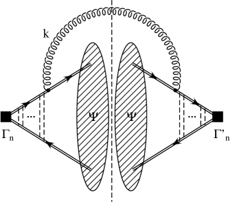
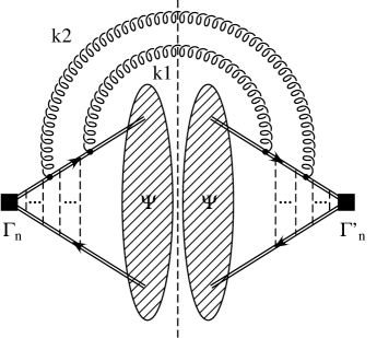
FIG. 3.: Left: one of four NRQCD diagrams which contribute to the M1 (E1) transition from an ${}^{1}\!S_{0}^{(8)}$ (${}^{3}\!P_{0}^{(8)}$) state, specified by $\Gamma_{n}^{(^{\prime})}$, to $J/\psi$. Right: an example for a double E1 transition from a ${}^{3}\!S_{1}^{(1,\,8)}$ state.

The non-relativistic quark-gluon vertices are classified according to their velocity suppression. The leading spin-flipping interaction is provided by the chromo-magnetic interaction vertex $-g_{s}/(2m_{c})(\mbox{\boldmath${\sigma}$}\times\mbox{\boldmath${k}$})$ with $k$ the outgoing gluon momentum as in Fig. 3. The diagram on the left hand side of Fig. 3 gives (cf. (6))

$$\frac{g_{s}^{2}C_{F}}{8m_{c}^{2}}\int\!\frac{d^{3}\mbox{\boldmath${k}$}}{(2\pi)^{3}2k^{0}}\left(\delta_{ij}-\frac{k_{i}k_{j}}{\mbox{\boldmath${k}$}^{2}}\right)\int\!\frac{d^{3}\mbox{\boldmath${p}$}}{(2\pi)^{3}}\frac{d^{3}\mbox{\boldmath${p}$}^{\prime}}{(2\pi)^{3}}\frac{d^{3}\mbox{\boldmath${q}$}}{(2\pi)^{3}}\frac{d^{3}\mbox{\boldmath${q}$}^{\prime}}{(2\pi)^{3}}$$ (47)

$$\hskip 28.45274pt\cdot\,\frac{1}{2}\sum_{\lambda}\mbox{tr}(\mbox{\boldmath${\epsilon}$}(\lambda)\!\cdot\!\mbox{\boldmath${\sigma}$}(\mbox{\boldmath${\sigma}$}\times\mbox{\boldmath${k}$})_{i})\,\mbox{tr}(\mbox{\boldmath${\epsilon}$}^{*}(\lambda)\!\cdot\!\mbox{\boldmath${\sigma}$}(\mbox{\boldmath${\sigma}$}\times(-\mbox{\boldmath${k}$}))_{j})\,\psi(\mbox{\boldmath${p}$})\,\psi(\mbox{\boldmath${p^{\prime}}$})$$ (48)

$$\hskip 28.45274pt\cdot\,iG_{c}(\mbox{\boldmath${p}$}+\mbox{\boldmath${k}$}/2,\mbox{\boldmath${q}$}+\mbox{\boldmath${k}$}/2;E(p_{R}+k))\,iG_{c}(\mbox{\boldmath${q}$}^{\prime}+\mbox{\boldmath${k}$}/2,\mbox{\boldmath${p}$}^{\prime}+\mbox{\boldmath${k}$}/2;E(p_{R}+k)),$$ (49)

with $\psi(\mbox{\boldmath${p}$})$ as given by (4) and $E(p_{R}+k)=p_{R}^{0}+k^{0}-2m_{c}=-m_{c}(C_{F}\alpha_{s})^{2}/4+k^{0}\equiv-\kappa^{2}/m_{c}$. Eq. (47) can be simplified, because the gluon is ultrasoft with energy and momentum of order $m_{c}v^{2}\sim m_{c}\alpha_{s}^{2}$, while ${p}$, $\mbox{\boldmath${p}$}^{\prime}$, ${q}$ and $\mbox{\boldmath${q}$}^{\prime}$ are of order $m_{c}v\sim m_{c}\alpha_{s}$. Dropping small terms in the arguments of the Coulomb Green function (as we have already done when defining $E(p_{R}+k)$), performing the traces and accounting for an identical contribution from the other three diagrams not shown in Fig. 3, we obtain

$$S[{}^{1}\!S_{0}^{(8)}](k;p_{R},P)=\frac{2g_{s}^{2}C_{F}}{m_{c}^{2}}\,\mbox{\boldmath${k}$}^{2}\left|I[{}^{1}\!S_{0}^{(8)}](k)\right|^{2},$$ (50)

where

$$I[^{1}\!S_{0}^{(8)}](k)=\int\!\frac{d^{3}\mbox{\boldmath${q}$}}{(2\pi)^{3}}\frac{d^{3}\mbox{\boldmath${p}$}}{(2\pi)^{3}}\,G_{c}(\mbox{\boldmath${q}$},\mbox{\boldmath${p}$};-\kappa^{2}/m_{c})\,\psi(\mbox{\boldmath${p}$}).$$ (51)

To compute this integral, we switch to coordinate space,

$$I[^{1}\!S_{0}^{(8)}](k)=\int\!d^{3}\mbox{\boldmath${x}$}\,\tilde{G}_{c}(\mbox{\boldmath${x}$},\mbox{\boldmath${0}$};-\kappa^{2}/m_{c})\,\tilde{\psi}(\mbox{\boldmath${x}$}),$$ (52)

use $\tilde{\psi}(\mbox{\boldmath${x}$})=\sqrt{\gamma^{3}/\pi}e^{-\gamma x}$ ($\gamma=m_{c}C_{F}\alpha_{s}/2$), gained by Fourier transformation of (4), and the following representation for the coordinate space Coulomb Green function [24]:

$$\tilde{G}_{c}(\mbox{\boldmath${x}$},\mbox{\boldmath${y}$};-\kappa^{2}/m_{c})=\sum_{l=0}^{\infty}\,(2l+1)\,\tilde{G}_{l}(x,y;-\kappa^{2}/m_{c})\,P_{l}(\mbox{\boldmath${x}$}\!\cdot\!\mbox{\boldmath${y}$}/(xy)),$$ (53)

where $x$, $y$ denote the modulus of ${x}$, ${y}$, $P_{l}(z)$ the Legendre polynomials and

$$\tilde{G}_{l}(x,y;-\kappa^{2}/m_{c})=\frac{m_{c}\kappa}{2\pi}\,(2\kappa x)^{l}(2\kappa y)^{l}e^{-\kappa(x+y)}\sum_{s=0}^{\infty}\frac{L_{s}^{(2l+1)}(2\kappa x)L_{s}^{(2l+1)}(2\kappa y)s!}{(s+l+1-\lambda\gamma/\kappa)(s+2l+1)!}.$$ (54)

Here $L_{s}^{(2l+1)}(z)$ refers to the Laguerre polynomials and the parameter $\lambda$ is defined such that the Green function corresponds to the Green function in the potential

$$V(r)=-\lambda\,\frac{C_{F}\alpha_{s}}{r}.$$ (55)

Hence $\lambda=1$, if the intermediate $c\bar{c}$ pair propagates in a colour singlet state, and $\lambda=-1/(2N_{c}C_{F})=-1/8$, if it propagates in a colour-octet state, which is what we need here. Only the $l=0$ component of the Green function contributes to the integral (52). The remaining radial integration over Laguerre polynomials is easily executed as an integral over the generating function

$$e^{-zu/(1-u)}\,\frac{1}{(1-u)^{p+1}}=\sum_{s=0}^{\infty}u^{s}\,L_{s}^{p}(z)$$ (56)

with subsequent expansion in $u$. Then, summing over $s$, and introducing the dimensionless variable

$$z=\kappa/\gamma=\left(1+\frac{4k_{0}}{m_{c}C_{F}^{2}\alpha_{s}^{2}}\right)^{\!1/2},$$ (57)

the result is

$$I[^{1}\!S_{0}^{(8)}](k) = -\frac{4m_{c}}{(\pi\gamma)^{1/2}}\frac{z^{2}}{(z^{2}-1)^{2}}\sum_{s=1}^{\infty}\frac{s\,(s-1/z)}{s-\lambda/z}\left(\frac{1-z}{1+z}\right)^{s}$$ (60)

$$=\,\frac{m_{c}}{(\pi\gamma)^{1/2}}\,\frac{1}{z^{2}-1}\,\Bigg{\{}\,1+(\lambda-1)\bigg{[}\frac{2}{z+1}$$

$$-\,\frac{4z}{z^{2}-1}\Big{(}1-{}_{2}F_{1}(-\lambda/z,1,1-\lambda/z;(1-z)/(1+z))\Big{)}\bigg{]}\Bigg{\}}$$

with ${}_{2}F_{1}(a,b,c;z)$ the hypergeometric function. Let us check the power counting: with $\gamma\sim m_{c}v$ and $k_{0},\,k_{i}\sim m_{c}v^{2}$, we obtain $I[^{1}\!S_{0}^{(8)}](k)\sim(m_{c}/v)^{1/2}$ and, from (46), (50), $\langle{\cal O}_{8}({}^{1}\!S_{0})\rangle\sim\alpha_{s}m_{c}^{3}v^{7}$. This agrees with the velocity power counting of [1]. The additional $\alpha_{s}$ arises, because we consider the weak coupling limit.

The chromo-electric dipole transition $c\bar{c}[{}^{3}\!P_{0}^{(8)}]\to J/\psi+g$ is computed along similar lines. We have

$$S[{}^{3}\!P_{0}^{(8)}](k;p_{R},P)=\frac{8g_{s}^{2}C_{F}}{3m_{c}^{4}}\,\left|I[{}^{3}\!P_{0}^{(8)}](k)\right|^{2},$$ (61)

where

$$I[^{3}\!P_{0}^{(8)}](k)=\frac{1}{3}\int\!d^{3}\mbox{\boldmath${x}$}\,\left[\frac{\partial}{\partial y_{i}}\,\tilde{G}_{c}(\mbox{\boldmath${x}$},\mbox{\boldmath${y}$};-\kappa^{2}/m_{c})\right]_{\mbox{\boldmath${y}$}=0}\,\frac{\partial}{\partial x_{i}}\tilde{\psi}(\mbox{\boldmath${x}$}),$$ (62)

and the normalization is given by

$$\int\!\frac{d^{3}\mbox{\boldmath${k}$}}{(2\pi)^{3}2k^{0}}\,S[{}^{3}\!P_{0}^{(8)}](k;p_{R},P)=\frac{\langle{\cal O}_{8}({}^{3}\!P_{0})\rangle}{m_{c}^{2}}.$$ (63)

The derivatives in (62) come from the factor ${p}$ in the electric dipole vertex $-ig_{s}(\mbox{\boldmath${p}$}+\mbox{\boldmath${p}$}^{\prime})/(2m_{c})\approx(-i)g_{s}\mbox{\boldmath${p}$}/m_{c}$. In this case only the $l=1$ component of the Green function survives the $\mbox{\boldmath${y}$}\to 0$ limit and the angular integration. The result is

$$I[^{3}\!P_{0}^{(8)}](k) = -\frac{4m_{c}\gamma^{3/2}}{3\pi^{1/2}}\,\frac{z^{3}}{(z+1)^{4}}\sum_{s=0}^{\infty}\frac{(s+1)(s+2)(s+3)}{s+2-\lambda/z}\,\left(\frac{1-z}{1+z}\right)^{\!s}$$ (67)

$$=\,\,-\frac{m_{c}\gamma^{3/2}}{3\pi^{1/2}}\,\frac{1}{(z+1)^{3}}\,\Bigg{\{}2(1+z)(2+z)+(\lambda-1)(5+3z)+2(\lambda-1)^{2}$$

$$+\,\frac{4z(1+z)(z^{2}-\lambda^{2})}{(1-z)^{2}}\bigg{[}{}_{2}F_{1}(-\lambda/z,1,1-\lambda/z;(1-z)/(1+z))-1$$

$$+\,\frac{\lambda(1-z)}{(1+z)(z-\lambda)}\bigg{]}\Bigg{\}}.$$

Velocity power counting gives $\langle{\cal O}_{8}({}^{3}\!P_{0})\rangle/m_{c}^{2}\sim\alpha_{s}m_{c}^{3}v^{7}$, which is again consistent with the standard counting.

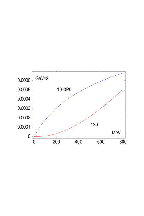
FIG. 4.: Dependence of $k_{0}/(4\pi^{2})\,S_{n}(k;p_{R},P)$ for $n={}^{1}\!S_{0}^{(8)}$ and $n={}^{3}\!P_{0}^{(8)}$ on the emitted gluon energy $k_{0}$. The parameters are chosen as $m_{c}=1.5\,$GeV, $\alpha_{s}=0.4$, $\lambda=-1/8$.

The dependence of $k_{0}/(4\pi^{2})\,S_{n}(k;p_{R},P)$ for $n={}^{1}\!S_{0}^{(8)}$ and $n={}^{3}\!P_{0}^{(8)}$ on the energy $k_{0}$ of the emitted gluon is shown in Fig. 4. The input parameters are chosen as $m_{c}=1.5\,$GeV, $\alpha_{s}=0.4$; $\lambda=-1/8$ for a colour octet matrix element. Both dependences are smooth and mainly reflect the asymptotic behaviours at small and large gluon energy. In particular the suppression of the ${}^{1}\!S_{0}$ curve at small $k_{0}$ is a consequence of the structure of the magnetic dipole vertex.

According to the normalization conditions (46) and (63) the integration of the two curves gives the value of the conventional NRQCD matrix elements. The result depends strongly (see the discussion below) on the cut-off on the integration range for $k_{0}$. Choosing the cut-off between $300\,$MeV and $600\,$MeV, we find

$$\langle{\cal O}_{8}^{J/\psi}({}^{1}\!S_{0})\rangle = (0.07-0.61)\cdot 10^{-4}\,\mbox{GeV}^{3}$$ (68)

$$\langle{\cal O}_{8}^{J/\psi}({}^{3}\!P_{0})\rangle/m_{c}^{2} = (0.07-0.22)\cdot 10^{-4}\,\mbox{GeV}^{3}.$$ (69)

Although these numbers may be insignificant, because the assumption $m_{c}v^{2}\gg\Lambda_{\rm QCD}$ necessary to obtain them, is not valid for charmonium, it is interesting to note that the matrix elements come out one to two orders of magnitude smaller than the phenomenological values, determined from fitting colour-octet subprocesses to experimental data [8]. This suggests either a large non-perturbative enhancement of the matrix elements – such as the presence of a gluon condensate to which the soft gluons can couple – or the possibility that the phenomenological values of the matrix elements effectively parametrize other corrections to the production processes not related to soft gluon emission (such as higher order short-distance corrections).

The behaviour of the soft function $S_{n}(k;p_{R},P)$ at large $k_{0}$ deserves further discussion. First, we observe that the calculation by itself does not provide an intrinsic cut-off for large $k_{0}$. This should not be expected, since at the level of perturbative radiation the ultraviolet behaviour of the soft function joins smoothly to the infrared behaviour of the short-distance part. A well known example of this occurs in $P$-wave production [1]: the logarithmic infrared behaviour of the coefficient function of $\langle{\cal O}_{1}^{\chi}(^{3}\!P_{0})\rangle$ matches the logarithmic ultraviolet divergence of $\langle{\cal O}_{8}^{\chi}(^{3}\!S_{1})\rangle$.

Inspection of $S[^{1}\!S_{0}^{(8)}](k;p_{R},P)$ shows that we obtain a quadratically ultraviolet divergent matrix element $\langle{\cal O}_{8}^{J/\psi}(^{1}\!S_{0})\rangle$, which seems to contradict the conventional wisdom that this matrix element is scale-independent at leading order. However, the conventional wisdom is derived from the use of dimensional regularization. If a hard cut-off on the gluon energy is used, the colour octet ${}^{1}\!S_{0}$ operator mixes into the colour singlet ${}^{3}\!S_{1}$ operator through a quadratically divergent term. This corresponds to a infrared finite, but quadratically infrared sensitive contribution to the coefficient function of $\langle{\cal O}_{1}^{J/\psi}(^{3}\!S_{1})\rangle$, consistent with the over-all $v^{4}$ suppression of $\langle{\cal O}_{8}^{J/\psi}(^{1}\!S_{0})\rangle$ relative to $\langle{\cal O}_{1}^{J/\psi}(^{3}\!S_{1})\rangle$. In dimensional regularization, the quadratically infrared sensitive term is attributed entirely to the short-distance coefficient and the quadratic divergence in $\langle{\cal O}_{8}^{J/\psi}(^{1}\!S_{0})\rangle$ is set to zero.

In case of $S[^{3}\!P_{0}^{(8)}](k;p_{R},P)$ we find a linear divergence for $\langle{\cal O}_{8}^{J/\psi}(^{3}\!P_{0})\rangle$. The interpretation of this divergence requires a more careful discussion of the $k_{0}$-integral and the integrals over ${p}$ and $\mbox{\boldmath${p}$}^{\prime}$; it will not be presented here.

In the ansatz (42) we have added a cut-off on $k_{0}$ by hand in the form of an exponential fall-off for $k_{0}\gg\Lambda_{n}$. We interpret this ansatz as a ‘primordial distribution’ for the radiation of non-perturbative gluons, which eventually is modified by perturbative evolution. This is similar to the assumption that intrinsic transverse momenta of the proton’s constituents are bounded. Perturbative radiation violates this assumption and leads to the evolution of parton distributions. A similar ansatz is also implied by the ACCMM model or in shape functions for semileptonic $B$ decays in general.

Finally, we comment on the transition from a colour octet or a colour singlet ${}^{3}\!S_{1}$ state to $J/\psi$. This presents a more complicated case, since – besides the contribution with no gluon emission for the colour singlet state – the leading term requires the emission of two gluons, see the right hand side of Fig. 3. In coordinate space this requires the evaluation of integrals of the form

$$I_{ij}[^{3}\!S_{1}^{(1,\,8)}] \sim \int\!d^{3}\mbox{\boldmath${x}$}d^{3}\mbox{\boldmath${y}$}\,\tilde{G}_{c}(-\mbox{\boldmath${y}$},\mbox{\boldmath${0}$};E(p_{R}+k_{1}))$$ (71)

$$\hskip 20.00003pt\times\left(\frac{\partial}{\partial y_{i}}\tilde{G}_{c}(\mbox{\boldmath${x}$},\mbox{\boldmath${y}$};E(p_{R}+k_{1}+k_{2}))\right)\left(\frac{\partial}{\partial x_{j}}\tilde{\psi}(\mbox{\boldmath${x}$})\right),$$

which we shall not pursue. If we were only interested in the limit of small loop momenta $k=k_{1}+k_{2}$, we could expand the Green functions for $k^{0}_{i}\ll\gamma^{2}/m_{c}$ first and integrate afterwards over ${x}$ and ${y}$. We would then find the same small-$k_{0}$ behaviour as in the case of $I[^{3}\!P_{0}](k)$.

III Momentum spectrum in $B\to J/\psi X$

In this section we apply the formalism developed in the previous section to the $J/\psi$ momentum spectrum in the semi-inclusive decay $B\to J/\psi X$. The leading partonic decay process is very simple, resulting in $J/\psi$ with fixed momentum, but the hadronic decay spectrum is modified by fragmentation of the $c\bar{c}$ pair, which is the main concern of this paper, and by bound state effects on the $b$ quark in the $B$ meson. Both will be taken into account in the following.

We start by recapitulating the partonic result for $b\to c\bar{c}[n]+q$. We then implement the fragmentation of the $c\bar{c}$ pair according to our shape function ansatz and obtain the $J/\psi$ momentum distribution in $b$ quark decay. We regard this distribution as input distribution for the ACCMM model, which accounts in a simple but satisfactory way for the effect of Fermi motion of the $b$ quark inside the $B$ meson. The resulting $J/\psi$ distribution in $B$ meson decay is then boosted to the CLEO frame and compared to CLEO data. The aim of this comparison is twofold: first we show that smearing of the spectrum due to fragmentation of the $c\bar{c}$ pair is essential to describe the CLEO data. Second we use these data to determine the shape function model parameter $\Lambda$. Assuming universality of the shape function over the whole kinematic domain, we will then turn to $J/\psi$ photoproduction in Sect. IV. Results for the $J/\psi$ momentum distributions already exist in the literature, including colour octet production [25, 26]. However, only Fermi motion effects are taken into account there. We will briefly compare our results with those of [25, 26] at the end of this section.

A Energy distribution in $b$ quark decay

The underlying partonic process of a $B$ meson decay into $J/\psi$ and light hadrons is $b\to c\bar{c}[n]+q$ ($q=\{d,s\}$). Since the $c\bar{c}$ pair is treated as a single particle kinematically a leading order calculation of this process results in a fixed value for its energy (momentum) rather than in a real spectrum. Defining $\hat{z}=2\hat{E}_{c\bar{c}}/m_{b}$ as the energy fraction of the $c\bar{c}$ pair in the $b$ quark rest frame, the “spectrum” is

$$\frac{d\Gamma_{\!\!c\bar{c}}}{d\hat{z}}=\Gamma_{\!\!c\bar{c}}\,\delta(1+\eta-\hat{z})\,,$$ (72)

where $\eta=4m_{c}^{2}/m_{b}^{2}$ for massless light hadrons in the final state. In a purely partonic calculation one may identify $2m_{c}$ with the $J/\psi$ mass and $m_{b}$ with the $B$ meson mass.

At leading order in the non-relativistic expansion the $c\bar{c}$ pair has to be produced in a colour singlet ${}^{3}S_{1}$ state. This term coincides with the colour singlet model and has been computed long ago [27, 28]. At relative order $v^{4}\approx 1/15$ in the non-relativistic expansion, $J/\psi$ can also be produced through $c\bar{c}$ in ${}^{1}S_{0}^{(8)},\,^{3}P_{J}^{(8)},\,^{3}S_{1}^{(8)}$ colour octet states. These formally subleading contributions are enhanced by a factor of about $15$, by which the short-distance structure of the $\Delta B=1$ weak effective Hamiltonian favours the production of colour octet $c\bar{c}$ pairs in the $b\to c\bar{c}q$ transition. These additional terms can be comparable or even larger than the colour singlet term [5, 6, 7]. They are the ones of interest in this paper, since the radiation of soft gluons in colour octet $c\bar{c}$ fragmentation has a large kinematic effect on the observed $J/\psi$ momentum spectrum. In comparison, fragmentation effects in the colour singlet channel are order $v^{4}$ suppressed relative to the total colour singlet rate and therefore negligible. Hard perturbative corrections to the colour singlet [7, 29] and colour octet [7] production processes are also known. They enhance the colour octet channels moderately. Within the present limitations of the shape function ansatz we must neglect these perturbative corrections for consistency. The partonic production spectra for the $c\bar{c}[n]$ states of interest read

$$\frac{d\Gamma_{\!\!c\bar{c}}[n]}{d\hat{z}}=\frac{1}{2m_{b}}\frac{1-\eta}{8\pi}\,H_{n}(m_{b},2m_{c})\,\delta(1+\eta-\hat{z}),$$ (73)

where

$$H_{n}(m_{b},2m_{c})=\frac{2G_{F}^{2}|V_{cb}|^{2}m_{b}^{4}}{27\pi(2m_{c})}\,C_{[1,8]}^{2}f[n](\eta)$$ (74)

and the process-specific functions $f[n](\eta)$ are given by [5, 6, 7]

$$f[^{3}S_{1}^{(1)}](\eta) = (1-\eta)(1+2\eta),$$ (75)

$$f[^{3}S_{1}^{(8)}](\eta) = \frac{3}{2}(1-\eta)(1+2\eta),$$ (76)

$$f[^{1}S_{0}^{(8)}](\eta) = \frac{9}{2}(1-\eta),$$ (77)

$$f[^{3}P_{J}^{(8)}](\eta) = 9(1-\eta)(1+2\eta).$$ (78)

Note that the colour octet matrix elements are not part of the hard amplitudes, but included in the normalization of the radiation function $\Phi_{n}(k)$, see (41). In case of the $P$ wave contribution, the normalization refers to $\langle{\cal O}_{8}({}^{3}P_{0})\rangle/m_{c}^{2}$ and the corresponding factor $1/m_{c}^{2}$ is also extracted from $H[^{3}P_{J}^{(8)}](m_{b},2m_{c})$. As mentioned above we neglect QCD corrections and also small corrections due to penguin operators. The Wilson coefficients $C_{[1,8]}$ of the effective operators in the weak $\Delta B=1$ Hamiltonian are related to the usual $C_{\pm}$ by

$$C_{[1]}(\mu) = 2C_{+}(\mu)-C_{-}(\mu),$$ (79)

$$C_{[8]}(\mu) = C_{+}(\mu)+C_{-}(\mu).$$ (80)

At leading order, as appropriate to the present analysis,

$$C_{\pm}(\mu)=\left[\frac{\alpha_{s}(M_{W})}{\alpha_{s}(\mu)}\right]^{\gamma_{\pm}^{(0)}/(2\beta_{0})}$$ (81)

with $\gamma_{\pm}^{(0)}=\mbox{}\pm 2(3\mp 1)$ and $\beta_{0}=11-2n_{f}/3$. In (74) the notation $C_{[1,8]}$ implies $C_{[1]}$, if $n$ is a colour-singlet state, and $C_{[8]}$, if $n$ is a colour octet state. Note that $C_{[8]}^{2}/C_{[1]}^{2}\approx 15$ at $\mu\sim m_{b}$.

We now implement $c\bar{c}$ fragmentation for the colour octet production channels. Notice that the partonic amplitude squared has no azimuthal dependence, hence $\bar{H}_{n}(m_{b},2m_{c})=H_{n}(m_{b},2m_{c})$ in the notation of (30). Furthermore, we need the light cone components of the incoming momentum $\hat{P}_{in}=(m_{b},\mbox{\boldmath${0}$})$ in the $J/\psi$ rest frame to get $\alpha$ and $\beta$ of (31). We find

$$\alpha=\frac{m_{b}}{M_{R}}(\hat{E}_{R}-|\hat{\mbox{\boldmath${p}$}}_{R}|)-M_{R},\qquad\beta=\frac{m_{b}}{M_{R}}(\hat{E}_{R}+|\hat{\mbox{\boldmath${p}$}}_{R}|)-M_{R}.$$ (82)

The index “R” now refers to $J/\psi$. To complete the implementation we have to fix the ambiguity in treating the kinematic effects in the hard production amplitudes $H_{n}$. Strictly speaking the shape function formalism allows us to ignore the dependence of the hard production process on the vector $l$, since it does not lead to singular contributions near the endpoint, if the hard matrix element is not singular at the endpoint. On the other hand, the invariant mass of the $c\bar{c}$ pair is kinematically given by

$$M^{2}_{c\bar{c}}(k)=(p+l)^{2}=(p_{R}+k)^{2}=M_{R}^{2}+2M_{R}k_{0}+k^{2},$$ (83)

where $k$ is the four momentum of soft radiation in the $J/\psi$ rest frame. We adopt the convention that $2m_{c}$ in the partonic matrix element is replaced by $M_{c\bar{c}}(k)$ everywhere, i.e. even when it does not arise kinematically, but through internal charm quark propagators. This convention is consistent with the shape function formalism in the shape function limit, but is arbitrary otherwise. It has the advantage of incorporating the physically expected effect of reducing the short-distance amplitude, because of the need to create a heavier $c\bar{c}$ pair as compared to a purely partonic picture. The only exception to the convention is the factor $1/(2m_{c})$ in (74), which comes from the normalization of the $c\bar{c}$ state. It should be replaced by $1/M_{R}$. Eq. (33), specialized to the $J/\psi$ energy distribution in $b$ quark decay, is then:

$$\frac{d\hat{\Gamma}}{d\hat{E}_{R}}=\frac{|\hat{\mbox{\boldmath${p}$}}_{R}|}{4\pi^{2}}\sum_{n}\int\limits_{0}^{\alpha\beta}\frac{dk^{2}}{2\pi}\!\int\limits_{(\alpha^{2}+k^{2})/(2\alpha)}^{(\beta^{2}+k^{2})/(2\beta)}\!\!\!dk_{0}\,\,\frac{1}{2m_{b}}\,H_{n}(m_{b},M_{c\bar{c}}(k))\,\frac{M_{R}}{8\pi m_{b}|\hat{\mbox{\boldmath${p}$}}_{R}|}\,\Phi_{n}(k)$$ (84)

with $\alpha$, $\beta$ from (82).

B Normalization difficulty

We assumed up to now that the radiation function $\Phi_{n}(k)$ is normalized according to (41). This implies that as $\Lambda$ of (42) tends to zero the integral over $d\hat{\Gamma}/d\hat{E}_{R}$ of (84) equals the integrated partonic rate with $m_{c}=M_{R}/2$.

Consider now the integral $\hat{\Gamma}_{n}(\Lambda)$ of the spectrum (84) with fragmentation (for a specific production channel $n$) at small $\Lambda$ and expand in $\Lambda$. To make things simpler put $k=0$ in the hard matrix element $H_{n}$. Then integrate over $\hat{E}_{R}$ or, equivalently, $\bar{z}\equiv 2\hat{E_{R}}/m_{b}$, and perform a change of variables from $\bar{z}$ to $\alpha$. Then note that for small $\Lambda$, one can set the upper limits of the $k^{2}$ and $k_{0}$ integrations to infinity up to exponentially small corrections in $\Lambda$, given the ansatz (42). Then exchange the $k^{2}$ and $k_{0}$ integration with the $\alpha$ integration to obtain

$$\hat{\Gamma}_{n}(\Lambda)=\frac{M_{R}}{16(2\pi)^{4}m_{b}}H_{n}(m_{b},M_{R})\int\limits_{0}^{\infty}dk^{2}\int\limits_{\sqrt{k^{2}}}^{\infty}dk_{0}\,\Phi_{n}(k)\!\!\!\int\limits_{k_{0}-\sqrt{k_{0}^{2}-k^{2}}}^{k_{0}+\sqrt{k_{0}^{2}-k^{2}}}\!\!\!d\alpha\,\left|\frac{d\bar{z}}{d\alpha}\right|.$$ (85)

Now introduce the average

$$\langle\langle f\rangle\rangle_{n}\equiv\frac{1}{(2\pi)^{3}}\,\frac{1}{\langle{\cal O}_{n}^{J/\psi}\rangle}\,\int\limits_{0}^{\infty}dk^{2}\int\limits_{\sqrt{k^{2}}}^{\infty}dk_{0}\,\sqrt{k_{0}^{2}-k^{2}}\,\Phi_{n}(k)\,f(k),$$ (86)

defined such that $\langle\langle 1\rangle\rangle_{n}=1$ according to the normalization condition (41). Eq. (85) is then rewritten in the form

$$\hat{\Gamma}_{n}(\Lambda)=\frac{1}{2m_{b}}\frac{1-\eta}{8\pi}\,H_{n}(m_{b},M_{R})\,\langle{\cal O}_{n}^{J/\psi}\rangle\cdot r_{n}(\Lambda),$$ (87)

where $\eta$ is now defined as $M_{R}^{2}/m_{b}^{2}$ and

$$r_{n}(\Lambda)=\frac{M_{R}}{2(1-\eta)}\,\langle\langle\,\frac{1}{\sqrt{k_{0}^{2}-k^{2}}}\!\!\!\!\int\limits_{k_{0}-\sqrt{k_{0}^{2}-k^{2}}}^{k_{0}+\sqrt{k_{0}^{2}-k^{2}}}\!\!\!\!\!\!d\alpha\,\left|\frac{d\bar{z}}{d\alpha}\right|\,\rangle\rangle_{n}.$$ (88)

Hence we obtain the partonic decay rate with $m_{c}=M_{R}/2$ up to the factor $r_{n}(\Lambda)$. To evaluate $r_{n}(\Lambda)$ in an expansion in $\Lambda$ we observe that

$$\left|\frac{d\bar{z}}{d\alpha}\right|=\frac{1}{M_{R}}\left(\frac{1}{(1+\alpha/M_{R})^{2}}-\eta\right)=\frac{1}{M_{R}}\left(1-\eta+\sum_{n=1}^{\infty}(n+1)\left(-\frac{\alpha}{M_{R}}\right)^{n}\right)$$ (89)

can be expanded under the integral. The result is

$$r_{n}(\Lambda)=1+\frac{1}{1-\eta}\left(-2\,\langle\langle\,\frac{k_{0}}{M_{R}}\,\rangle\rangle_{n}+\langle\langle\,\frac{4k_{0}^{2}-k^{2}}{M_{R}^{2}}\,\rangle\rangle_{n}+O\left(\frac{\Lambda^{3}}{M_{R}^{3}}\right)\right).$$ (90)

The averages can be done using (42) with $a_{n}$ fixed by (41); they scale with definite powers of $\Lambda$ as follows from the form of (86). With $\eta=0.416$, the result is

$$r_{n}(\Lambda)=1-\left\{\begin{array}[]{cc}4.76\\ 5.75\end{array}\right\}\frac{\Lambda}{M_{R}}+\left\{\begin{array}[]{cc}12.97\\ 19.53\end{array}\right\}\left(\frac{\Lambda}{M_{R}}\right)^{2}+\ldots,$$ (91)

where the upper number refers to $b_{n}=0$ in (42) and the lower one to $b_{n}=2$. For $\Lambda\approx 300\,$MeV this implies large corrections to the integrated rate. Since $\Lambda\sim m_{c}v^{2}$, this must be interpreted as large higher order corrections in the velocity expansion, which are not taken into account in the usual leading order NRQCD analysis. This means that enforcing the normalization condition (41) underestimates the data, because the matrix elements on the right hand side of (41) have been obtained without these large higher order corrections.

The effect is in fact even larger than indicated by (91), because we keep the $k$ dependence of the hard matrix element and $M_{c\bar{c}}(k)$ is always larger than $M_{R}$. As an indication of this effect we can compute the average

$$4{m_{c}^{\rm eff}}^{2}\equiv\langle\langle\,M_{c\bar{c}}(k)^{2}\,\rangle\rangle_{n}\approx M_{R}^{2}\left(1+\left\{\begin{array}[]{cc}2.78\\ 3.39\end{array}\right\}\frac{\Lambda}{M_{R}}\right)$$ (92)

which implies an effective charm quark mass of about $1.8\,$GeV rather than $m_{c}=1.5\,$GeV which is usually adopted in partonic NRQCD calculations.

When the implicit $k$-dependence of the partonic matrix element $H_{n}$ is taken into account, the numbers given in (91) change. However, the observation that $v^{2}$ corrections are large is generic.

C Fermi motion effects

We now convert the spectrum (84) in $b$ quark decay into a spectrum in $B$ meson decay by accounting for Fermi motion of the $b$ quark. We make the reasonable assumption that $B$ meson bound state effects can be factorized from the hard subprocess as well as from $c\bar{c}$ fragmentation. The Fermi motion effect can be described rigorously in heavy quark effective theory [19], but we contend ourselves with the earlier ACCMM model [21]. The ACCMM model is in fact consistent with the heavy quark expansion, if a particular relation between the $b$ quark mass and the ACCMM model parameter $p_{F}$ is adopted [30]. (The ACCMM model then assumes a particular value for the kinetic energy matrix element of heavy quark effective theory.) The ACCMM model provides a phenomenologically viable description of energy spectra in other $B$ decays, e.g. $B\to X\ell\bar{\nu}_{\ell}$ or $B\to X_{s}\gamma$.

The basic idea of this model is quite intuitive: one imagines the $b$ quark moving inside the $B$ meson at rest with a momentum $p$ according to some distribution with a width of a few hundred MeV. The cloud of gluons and light quarks in the $B$ meson of the mass $M_{B}$ is treated as spectator quark with mass $m_{sp}$. To keep the kinematics of this “decay in flight” exact one introduces a so-called floating $b$ quark mass

$$m_{b}^{2}(p)=M_{B}^{2}+m_{sp}^{2}-2M_{B}\sqrt{m_{sp}^{2}+p^{2}}.$$ (93)

The $b$ quark is on-shell with energy $E_{b}(p)=(m_{b}^{2}(p)+p^{2})^{1/2}$. The $b$ quark momentum distribution must be chosen ad hoc. Usually one takes a properly normalized Gaussian form

$$\Phi_{\rm ACM}(p)=\frac{4}{\sqrt{\pi}p_{F}^{3}}\exp\,(-p^{2}/p_{F}^{2}),$$ (94)

where $\int_{0}^{\infty}dp\,p^{2}\,\Phi_{\rm ACM}(p)=1$. Implementing the kinematics of decay in flight, the $J/\psi$ energy distribution in the $B$ meson rest frame (quantities without “hat”) is then obtained from the spectrum in $b$ quark decay (84) by the convolution

$$\frac{d\Gamma}{dE_{R}}=\int\limits_{\max\{0,\,p_{-}\}}^{p_{+}}\!\!\!\!\!dp\,p^{2}\,\Phi_{\rm ACM}(p)\frac{m_{b}^{2}(p)}{2pE_{b}(p)}\int\limits_{\hat{E}_{R}^{\rm min}(p)}^{\hat{E}_{R}^{\rm max}(p)}\frac{d\hat{E}_{R}}{\hat{E}_{R}}\frac{d\hat{\Gamma}}{d\hat{E}_{R}}.$$ (95)

The integration over the $J/\psi$ energy $\hat{E}_{R}$ in the $b$ quark rest frame is limited by

$$\hat{E}_{R}^{\rm max} = \min\left\{\frac{E_{R}E_{b}(p)+|\mbox{\boldmath${p}$}_{R}|p}{m_{b}(p)},\,\frac{m_{b}^{2}(p)+M_{R}^{2}}{2m_{b}(p)}\right\},$$ (96)

$$\hat{E}_{R}^{\rm min} = \frac{E_{R}E_{b}(p)-|\mbox{\boldmath${p}$}_{R}|p}{m_{b}(p)}.$$ (97)

The requirement $\hat{E}_{R}^{\rm min}\leq{E}_{R}^{\rm max}$ leads to the following bounds on $p$:

$$p_{\pm}=\frac{[p_{R}\pm(M_{B}-E_{R})]^{2}-m_{sp}^{2}}{2[p_{R}\pm(M_{B}-E_{R})]}.$$ (98)

The dependence of the energy spectrum (95) on the two parameters of the ACCMM model, $m_{sp}$ and $p_{F}$, is quite different. Changing the value of the spectator mass does not affect the spectrum noticeably. Therefore $m_{sp}$ usually is fixed to 150 MeV in all ACCMM analyses. On the other hand the width $p_{F}$ of the momentum distribution must be chosen carefully, because the shape of the spectrum is strongly sensitive to this parameter. Successful fits to the lepton energy spectrum in semi-leptonic decay typically find $p_{F}\approx(300-450)\,$ MeV [31].

D Final result and comparison with CLEO data

Eq. (95) yields the $J/\psi$ energy spectrum for $B$ mesons decaying at rest. To compare with CLEO data [16], we have to translate the energy spectrum (95) into a momentum spectrum

$$\frac{d\Gamma}{dp_{R}}=\frac{E_{R}}{p_{R}}\,\frac{d\Gamma}{dE_{R}}$$ (99)

and account for the fact that $B$ mesons have momentum $\tilde{p}_{B}=(M_{\Upsilon(4S)}^{2}/4-M_{B}^{2})^{1/2}\approx 482\,$MeV in the CLEO rest frame in which the data in [16] is presented. The final boost from the $B$ meson to the $\Upsilon(4S)$ rest frame is effected by

$$\frac{d\tilde{\Gamma}}{d\tilde{p}_{R}}=\frac{\tilde{p}_{R}}{\tilde{E}_{R}}\,\frac{M_{B}}{2\tilde{p}_{B}}\int\limits_{p_{R}^{\rm min}}^{p_{R}^{\rm max}}\!\!\frac{dp_{R}}{p_{R}}\,\frac{d\Gamma}{dp_{R}}\,,$$ (100)

where the bounds on the $J/\psi$ momentum

$$p_{R}^{\rm min} = \max\left\{0,\frac{\tilde{E}_{B}\tilde{p}_{R}-\tilde{p}_{B}\tilde{E}_{R}}{M_{B}}\right\}\,,$$ (101)

$$p_{R}^{\rm max} = \min\left\{\frac{\lambda^{1/2}(M_{B}^{2},M_{R}^{2},m_{sp}^{2})}{2M_{B}},\frac{\tilde{E}_{B}\tilde{p}_{R}+\tilde{p}_{B}\tilde{E}_{R}}{M_{B}}\right\}$$ (102)

stem from kinematical restrictions set by the masses in the Källen function $\lambda(x,y,z)=x^{2}+y^{2}+z^{2}-2xy-2xz-2yz$ and from the integration over the angle between the $B$ and the $J/\psi$ momentum.

Owing to the difficulties of normalizing the partial production rates discussed above we forsake the idea of predicting the absolute $J/\psi$ branching fraction in $B$ decay and concentrate on the shape of the spectrum. We fix the absolute normalization by adjusting the sum of all contributions to data. This is actually equivalent to re-fitting the NRQCD matrix elements to data after including large higher order corrections in the velocity expansion. However, we do not give the result of the re-fitting, because we believe it is of little interest for comparison with other $J/\psi$ production processes.

The shape function ansatz (42) is slightly different for the different production channels because of the different choice of parameters (43), (44). Therefore the shape of the momentum spectrum depends somewhat on the relative contribution of the various channels even after adjusting the overall normalization to data. We determine the relative normalization of the various channels by comparing the existing information on the NRQCD matrix elements obtained by standard leading order NRQCD analyses. The colour singlet matrix element can be computed from the wave function at the origin. The Buchmüller-Tye potential is often adopted with the result [32]

$$\langle{\cal O}^{J/\psi}_{1}(^{3}\!S_{1})\rangle=\frac{9|R(0)|^{2}}{2\pi}=1.16\,\mbox{GeV}^{3}.$$ (103)

Due to our particular treatment of the colour singlet contribution as described below, we do not need this matrix element in $B$ decay. The colour octet matrix elements are determined by fits to $J/\psi$ production in a variety of production processes. $\langle{\cal O}^{J/\psi}_{8}(^{3}\!S_{1})\rangle$ is best determined from $J/\psi$ production in hadron-hadron collisions at large transverse momentum [2, 33, 12], or, perhaps, from charmonium production in $Z^{0}$ decays [34]. Given uncertainties from unknown higher order perturbative corrections a reasonable range is

$$\langle{\cal O}^{J/\psi}_{8}(^{3}\!S_{1})\rangle=(0.5-1.0)\cdot 10^{-2}\,\mbox{GeV}^{3}.$$ (104)

The determination of the other two matrix elements from hadron-hadron collisions is much more uncertain. Assuming the above range for $\langle{\cal O}^{J/\psi}_{8}(^{3}\!S_{1})\rangle$ a significant constraint on

$$M_{k}^{J/\psi}(^{1}\!S_{0}^{(8)},^{3}\!P_{0}^{(8)})=\langle{\cal O}^{J/\psi}_{8}(^{1}S_{0})\rangle+\frac{k}{m_{c}^{2}}\langle{\cal O}^{J/\psi}_{8}(^{3}P_{0})\rangle\,.$$ (105)

with $k=3.1$ arises from the integrated $J/\psi$ branching in $B$ decay itself [7]. A reasonable range is

$$M_{3.1}^{J/\psi}(^{1}\!S_{0}^{(8)},^{3}\!P_{0}^{(8)})=(1.0-2.0)\cdot 10^{-2}\,\mbox{GeV}^{3}.$$ (106)

As default we take the value $M_{3.1}^{J/\psi}=1.5\cdot 10^{-2}\,\mbox{GeV}^{3}$ for $m_{c}=1.5\,\mbox{GeV}$ and assume that it originates from both parts equally. We then investigate the modification of the spectrum when $M_{3.1}^{J/\psi}(^{1}\!S_{0}^{(8)},^{3}\!P_{0}^{(8)})$ is saturated by only one of the two matrix elements and when the relative contribution of $\langle{\cal O}^{J/\psi}_{8}(^{3}\!S_{1})\rangle$ and $M_{3.1}^{J/\psi}(^{1}\!S_{0}^{(8)},^{3}\!P_{0}^{(8)})$ is varied as allowed by the ranges of values given. At the end we discard the absolute normalization that would be implied by these values and re-fit it to data as already mentioned.

A final comment concerns the treatment of the two-body modes $B\to J/\psi K$ and $B\to J/\psi K^{*}$, which appear as sharp resonances in the $J/\psi$ momentum spectrum. Neither the ACCMM model nor the shape function for $c\bar{c}$ fragmentation applies to these resonance contributions. Fortunately, the information provided in [16] allows us to subtract these contributions from the momentum spectrum. We then assume that the two resonant contributions are dual to the colour singlet contribution, while the rest of the spectrum corresponds to the colour octet contribution. This appears plausible, because we expect colour octet $c\bar{c}$ pairs to fragment into multi-body final states, with only a small probability that the emitted soft gluons reassemble with the spectator quark to form a single hadron. Hence, the experimental spectrum shown in the following plots refers to the CLEO data with $B\to J/\psi K$ and $B\to J/\psi K^{*}$ subtracted and it is compared with colour octet contributions only. The integrated branching fraction from the resonance subtracted spectrum is $0.53\,\%$. Of course, indirect contributions from $B\to\psi^{\prime}X$ and $B\to\chi_{c}X$ with subsequent decay into $J/\psi$ are also subtracted.

FIG. 5.: Sum of colour octet modes $d{\rm BR}_{[8]}/dp_{R}[n]$ with $n=\{^{1}\!S_{0}^{(8)},\,^{3}\!P_{0}^{(8)},\,^{3}\!S_{1}^{(8)}\}$ to the differential branching ratio $d{\rm BR}/dp_{R}$ of the decay $B\to J/\psi X$ for various values of the shape function parameter $\Lambda$. The ACCMM model parameters are fixed at $p_{F}=300$ GeV and $m_{sp}=150$ GeV.

We have implemented the five-fold integration that leads to the final $J/\psi$ momentum spectrum into a Monte Carlo program that uses the VEGAS routine described in [35]. Parameters are chosen as follows: $G_{F}=1.166\cdot 10^{-5}\,\mbox{GeV}^{-2}$, $|V_{cb}|=0.039$, $M_{\Upsilon}=10.580\,\mbox{GeV}$, $M_{B}=5.279\,\mbox{GeV}$ and $M_{\psi}=3.097\,\mbox{GeV}$. The Wilson coefficient $C_{[8]}(\mu)$ is taken at the scale $\mu=4.8$ GeV, which yields $C_{[8]}=2.19$. The result compared to data is shown in Fig. 5 for various values of the shape function parameter $\Lambda$ (see the ansatz (42) and (44)). Here we have fixed the ACCMM model parameters to $p_{F}=300$ MeV, motivated by the CLEO analysis of semi-leptonic $B$ decay [31], and $m_{sp}=150$ MeV. It is clearly seen that the effect of $c\bar{c}$ fragmentation is necessary to reproduce the data for this choice of ACCMM parameters. Increasing $\Lambda$ shifts the maximum of the spectrum to lower values of $p_{R}$. We get the best fit for $\Lambda=300$ MeV, where $\chi^{2}=30.2/20$ d.o.f..

FIG. 6.: Contributions of the different colour octet modes $n=\{^{1}\!S_{0}^{(8)},\,^{3}\!P_{J}^{(8)},\,^{3}\!S_{1}^{(8)}\}$ to the sum $d{\rm BR}/dp_{R}$ of the differential branching ratio. The shape function and the ACCMM parameters are fixed to $\Lambda=300$ MeV, $p_{F}=300$ MeV and $m_{sp}=150$ MeV.

In order to estimate the uncertainty of this fit we investigated the sensitivity of the best-fit $\Lambda$ to the variation of the relative normalization of the various $c\bar{c}$ production channels as described above and to the ACCMM parameter $p_{F}$. Fig. 6 shows the best-fit result of Fig. 5 broken down into the separate contributions of the three colour octet channels. Each channel peaks approximately at the same value $p_{R}$ and has similar shapes, although the ${}^{3}\!S_{1}$ contribution is somewhat broader due to the choice of $c=1.5$ in (44). (Varying $c$ between 1 and 2 does not change our fit significantly.) Thus the result of fitting $\Lambda$ is rather stable under changing the weightings of the different modes. Both, increasing the relative contribution of $M_{3.1}^{J/\psi}$ and saturating it by only one of its matrix elements leads to variations of $\Lambda$ of about 50 MeV. There is an obvious anti-correlation between the size of $\Lambda$ and of $p_{F}$, although the effect is not as large as one may expect. Figure 7 shows the spectra for different values of $p_{F}$ while $\Lambda$ is fixed to 300 MeV. We obtain that the spectrum is slightly wider for higher values of $p_{F}$. But even for $p_{F}=500$ MeV the best-fit $\Lambda$ would remain of order 200 MeV.

FIG. 7.: Sum of colour octet modes $d{\rm BR}_{[8]}/dp_{R}[n]$ with $n=\{^{1}\!S_{0}^{(8)},\,^{3}\!P_{0}^{(8)},\,^{3}\!S_{1}^{(8)}\}$ to the differential branching ratio $d{\rm BR}/dp_{R}$ of the decay $B\to J/\psi X$ for various values of the ACCMM parameter $p_{F}$. The shape function parameter $\Lambda=300$ MeV and the spectator mass $m_{sp}=150$ of the ACCMM model are kept fixed.

We conclude from this analysis that the kinematics of soft gluon emission has to be accounted for to describe the data on $J/\psi$ momentum spectra and that our shape function model provides a satisfactory description of the spectrum shape, if the parameter $\Lambda$ is chosen in the range

$$\Lambda=300^{+50}_{-100}\,\mbox{MeV}.$$ (107)

This result agrees perfectly with the velocity scaling rules, which lead to the estimate $\Lambda\sim m_{c}v^{2}\sim\Lambda_{\rm QCD}$. It is also worth noting that the partonic spectrum behind Fig. 5 is a pure delta-function so that the smearing due to $c\bar{c}$ fragmentation and Fermi motion extends almost over the entire accessible momentum range. Only for rather small $J/\psi$ momentum, there would be a visible tail due to perturbative hard gluon radiation [7].

Finally let us comment on the $J/\psi$ momentum spectra in [25, 26] based on the effect of Fermi motion only. (Earlier results [36] were based on the colour singlet model and will not be discussed.) These works also report acceptable fits of the $J/\psi$ momentum spectrum, however with a larger value of $p_{F}\approx 550\,$MeV, as one may expect when $c\bar{c}$ fragmentation effects are neglected. However, even this large value of $p_{F}$ is obtained only, because the $K$ and $K^{*}$ resonances, which sit at large values of $p_{R}$ have been included, even though the ACCMM model cannot be applied to them. If these contributions are subtracted, as done in the present analysis, a satisfactory fit is not obtained with the ACCMM model alone.

IV Inelastic $J/\psi$ photoproduction

In this section we discuss the energy spectrum in inelastic $J/\psi$ photoproduction. This is perhaps the most interesting application of the shape function model developed in this paper. The colour octet contributions to the energy spectrum have been predicted to increase rapidly in the endpoint region, where the $J/\psi$ approaches its maximal kinematically allowed energy [9, 37]. If the colour octet matrix elements take the values required to fit the normalization of production cross sections in hadron-hadron collisions and in $B$ decay, this prediction contradicts the data collected at the HERA collider [10], which show a rather flat energy distribution. The measured distribution can in principle be described by colour singlet contributions alone, both at leading order and at next-to-leading order [38] in $\alpha_{s}$.

Several solutions have been proposed to solve this problem for the NRQCD approach to charmonium production:

(a) The relevant colour octet matrix elements are smaller than believed [39]. The colour octet contributions are always small and the shape of the energy spectrum is determined by the colour singlet term.

(b) The partonic cross section is modified by intrinsic transverse momentum effects. Within a particular model for these effects [40] obtains a reduction of the colour octet cross section, while the energy dependence is essentially unmodified.

(c) The NRQCD calculation is unreliable for large $J/\psi$ energies because of a breakdown of the non-relativistic expansion [18]. Resummation of the expansion as discussed earlier leads to folding the partonic cross section with a shape function. It is expected that this leads to a depression of the spectrum at large $J/\psi$ energies, because some energy is lost for radiation in the fragmentation of the colour octet $c\bar{c}$ pair.

In this section we pursue suggestion (c), which has not been implemented in practice yet. Let us note that, irrespective of the issue of normalization, this is the only solution that addresses the fact that the shape of the colour octet spectrum obtained from a partonic calculation is unphysical for large $J/\psi$ energies.

The section is organized as follows. In parallel with the discussion of the $B$ decay we begin with kinematics and by listing the relevant partonic subprocesses $\gamma+g\to c\bar{c}[n]+g$. We then incorporate the fragmentation of the $c\bar{c}$ pair via our shape function ansatz and discuss the modification of the energy spectrum. For the sake of demonstration, we compare the result to HERA data, although we shall see that this comparison is problematic from a theoretical point of view.

A Kinematics of photoproduction

The quantity of interest is $d\sigma/dz$, where

$$z=\frac{p_{R}\cdot p_{p}}{p_{\gamma}\cdot p_{p}},$$ (108)

and $p_{R}$, $p_{p}$ and $p_{\gamma}$ denote the $J/\psi$, proton and photon momentum, respectively. In the proton rest frame $z$ is the fraction of the photon energy transferred to the $J/\psi$. In the photon-proton centre-of-mass system (cms) we define

$$p_{\gamma} = \frac{\sqrt{s}}{2}\,(1,0,0,-1),$$ (109)

$$p_{g} = x_{g}p_{p}=x_{g}\frac{\sqrt{s}}{2}\,(1,0,0,+1),$$ (110)

$$p_{R} = (E_{R},p_{T},0,p_{R}^{z}),$$ (111)

where $s=(p_{p}+p_{\gamma})^{2}$ is the cms energy and $x_{g}$ the gluon momentum fraction of the proton momentum. Note that $z$ and $p_{T}$ refer to the physical $J/\psi$ particle. In the present context they cannot be identified with the corresponding quantities of the progenitor $c\bar{c}$ pair, which we denote by $z_{c\bar{c}}$ and $p_{T,c\bar{c}}$. Using $p_{R}^{2}=M_{R}^{2}$, we express the $J/\psi$ energy $E_{R}$ and its longitudinal momentum $p_{R}^{z}$ in terms of its transverse momentum $p_{T}$ and $z$:

$$E_{R}=\frac{z^{2}s+p_{T}^{2}+M_{R}^{2}}{2z\sqrt{s}},\qquad p_{R}^{z}=-\frac{z^{2}s-p_{T}^{2}-M_{R}^{2}}{2z\sqrt{s}}.$$ (112)

The convolution with the shape function, (33), requires $\alpha$ and $\beta$, defined by (31) in the quarkonium rest frame. According to our convention, the $\hat{z}$-axis is defined in the direction of $-\hat{\mbox{\boldmath${P}$}}_{in}$ with $\hat{\mbox{\boldmath${P}$}}_{in}=\hat{\mbox{\boldmath${p}$}}_{\gamma}+\hat{\mbox{\boldmath${p}$}}_{g}$. Writing

$$\hat{p}_{\gamma} = \left(\hat{E}_{\gamma},\;\hat{p}_{\perp},\;0,\;\hat{p}_{\gamma}^{z}\right),$$ (113)

$$\hat{p}_{g} = \left(\hat{E}_{g},\;-\hat{p}_{\perp},\;0,\;\hat{p}_{g}^{z}\right),$$ (114)

$$\hat{P}_{in} = \left(\hat{E}_{in},\;0,\;0,\;\hat{P}_{in}^{z}\right),$$ (115)

and performing the Lorentz transformation explicitly, we obtain

$$\hat{E}_{\gamma} = \frac{M_{R}^{2}+p_{T}^{2}}{2M_{R}z},$$ (116)

$$\hat{p}_{\perp} = \frac{p_{T}zx_{g}s}{\lambda^{1/2}(M_{R}^{2},-p_{T}^{2},x_{g}sz^{2})},$$ (117)

$$\hat{p}_{\gamma}^{z} = -\frac{z^{2}x_{g}s(p_{T}^{2}-M_{R}^{2})+(p_{T}^{2}+M_{R}^{2})^{2}}{2zM_{R}\lambda^{1/2}(M_{R}^{2},-p_{T}^{2},x_{g}sz^{2})},$$ (118)

$$\hat{E}_{g} = \frac{zx_{g}s}{2M_{R}},$$ (119)

$$\hat{p}_{g}^{z} = -\frac{zx_{g}s(z^{2}x_{g}s+p_{T}^{2}-M_{R}^{2})}{2M_{R}\lambda^{1/2}(M_{R}^{2},-p_{T}^{2},x_{g}sz^{2})}$$ (120)

with $\lambda(x,y,z)=x^{2}+y^{2}+z^{2}-2xy-2xz-2yz$, and

$$\hat{E}_{in}=\frac{M_{R}^{2}+p_{T}^{2}+x_{g}sz^{2}}{2M_{R}z},\qquad\hat{P}_{in}^{z}=-\frac{\lambda^{1/2}(M_{R}^{2},-p_{T}^{2},x_{g}sz^{2})}{2M_{R}z}.$$ (121)

The previous line gives $\alpha$ and $\beta$, defined as

$$\alpha=\hat{E}_{in}+\hat{P}_{in}^{z}-M_{R},\qquad\beta=\hat{E}_{in}-\hat{P}_{in}^{z}-M_{R}$$ (122)

for given $z$ and $p_{T}$ of the $J/\psi$ in the cms frame.

The Mandelstam variables that appear in the hard production amplitude for $\gamma+g\to c\bar{c}[n]+g$ are defined as

$$\hat{s} = (\hat{p}_{g}+\hat{p}_{\gamma})^{2}=x_{g}s,$$ (123)

$$\hat{t} = (\hat{p}_{c\bar{c}}-\hat{p}_{\gamma})^{2},$$ (124)

$$\hat{u} = (\hat{p}_{c\bar{c}}-\hat{p}_{g})^{2}.$$ (125)

We have to express them in terms of $z$, $p_{T}$, $x_{g}$ and the energy $\hat{k}_{0}$ and invariant mass $\hat{k^{2}}$ of the radiated soft partons in the $J/\psi$ rest frame. Recall that $\hat{p}_{c\bar{c}}\equiv\hat{P}+\hat{l}=\hat{p}_{R}+\hat{k}$ with $\hat{P}=(2m_{c},\mbox{\boldmath${0}$})$. Hence

$$\hat{u}=M_{c\bar{c}}(k)^{2}-\hat{s}-\hat{t},$$ (126)

where $M_{c\bar{c}}(k)^{2}=M_{R}^{2}+2M_{R}\hat{k}_{0}+\hat{k}^{2}$ as usual. Next parametrize the momentum of the $c\bar{c}$ pair by

$$\hat{p}_{c\bar{c}}=\left(\hat{E}_{c\bar{c}},\;\hat{l}_{\perp}\cos\hat{\phi},\;\hat{l}_{\perp}\sin\hat{\phi},\hat{l}_{z}\right).$$ (127)

This introduces azimuthal angular dependence into the partonic matrix element. This dependence is formally small. All $\hat{\phi}$ dependent terms are proportional to $\hat{l}_{\perp}$, and, as discussed in Sect. II B 2, such transverse momentum dependence can be neglected in the strict shape function limit. In our ansatz, which models the entire spectrum, we also have to keep the exact kinematic relations and therefore a non-trivial azimuthal average of the hard production amplitude appears in this case. With the help of on-shell conditions for the hard emitted gluon we can express the components of $\hat{p}_{c\bar{c}}$ by

$$\hat{E}_{c\bar{c}} = M_{R}+\hat{k}_{0},$$ (128)

$$\hat{l}_{\perp} = \hat{k}_{\perp}=\frac{[\hat{k}^{2}-\alpha(2\hat{k}_{0}-\alpha)]^{1/2}[\beta(2\hat{k}_{0}-\beta)-\hat{k}^{2}]^{1/2}}{\beta-\alpha},$$ (129)

$$\hat{l}_{z} = \hat{k}_{z}=\frac{\hat{k}^{2}+\alpha\beta-\hat{k}_{0}(\alpha+\beta)}{\beta-\alpha}.$$ (130)

This result, together with the result for $\hat{p}_{\gamma}$ and $\alpha$, $\beta$, allows us to express $\hat{t}$ in terms of $z$, $p_{T}$, $\hat{k}_{0}$, $\hat{k}^{2}$ and $x_{g}$.

Let us now turn to the hard amplitudes squared of the partonic subprocesses. We restrict ourselves to photon-gluon fusion, $\gamma+g\to c\bar{c}[n]+g$, where $n$ represents either the dominant colour singlet state ${}^{3}S_{1}$ or one of the colour octet states ${}^{1}S_{0}$, ${}^{3}P_{J}$, ${}^{3}S_{1}$. In terms of Mandelstam variables, the spin averaged expressions are [9, 37, 41]:

$$H[^{3}S_{1}^{(1)}](\hat{s},\hat{t},\hat{u},2m_{c}) = \frac{16e_{c}^{2}e^{2}g_{s}^{2}(2m_{c})\left[\hat{s}^{2}(\hat{t}+\hat{u})^{2}+\hat{t}^{2}(\hat{u}+\hat{s})^{2}+\hat{u}^{2}(\hat{s}+\hat{t})^{2}\right]}{27(\hat{s}+\hat{t})^{2}(\hat{t}+\hat{u})^{2}(\hat{u}+\hat{s})^{2}},$$ (131)

$$H[^{1}S_{0}^{(8)}](\hat{s},\hat{t},\hat{u},2m_{c}) = \frac{3e_{c}^{2}e^{2}g_{s}^{2}\hat{s}\hat{u}\left[(\hat{s}+\hat{t}+\hat{u})^{4}+\hat{s}^{4}+\hat{t}^{4}+\hat{u}^{4}\right]}{(2m_{c})\hat{t}(\hat{s}+\hat{t})^{2}(\hat{t}+\hat{u})^{2}(\hat{u}+\hat{s})^{2}},$$ (132)

$$H[^{3}P_{J}^{(8)}](\hat{s},\hat{t},\hat{u},2m_{c}) = \frac{6e_{c}^{2}e^{2}g_{s}^{2}}{(2m_{c})\hat{t}(\hat{s}+\hat{t})^{3}(\hat{t}+\hat{u})^{3}(\hat{u}+\hat{s})^{3}}$$ (140)

$$\mbox{}\times\Big{[}\hat{t}^{6}(2\hat{s}^{3}+13\hat{s}^{2}\hat{u}+13\hat{s}\hat{u}^{2}+2\hat{u}^{3})$$

$$\mbox{}+\hat{t}^{5}(4\hat{s}^{4}+47\hat{s}^{3}\hat{u}+70\hat{s}^{2}\hat{u}^{2}+47\hat{s}\hat{u}^{3}+4\hat{u}^{4})$$

$$\mbox{}+\hat{t}^{4}(2\hat{s}^{5}+63\hat{s}^{4}\hat{u}+136\hat{s}^{3}\hat{u}^{2}+136\hat{s}^{2}\hat{u}^{3}+63\hat{s}\hat{u}^{4}+2\hat{u}^{5})$$

$$\mbox{}+\hat{s}\hat{t}^{3}\hat{u}(47\hat{s}^{4}+132\hat{s}^{3}\hat{u}+190\hat{s}^{2}\hat{u}^{2}+132\hat{s}\hat{u}^{3}+47\hat{u}^{4})$$

$$\mbox{}+\hat{s}\hat{t}^{2}\hat{u}(25\hat{s}^{5}+88\hat{s}^{4}\hat{u}+156\hat{s}^{3}\hat{u}^{2}+156\hat{s}^{2}\hat{u}^{3}+88\hat{s}\hat{u}^{4}+25\hat{u}^{5})$$

$$\mbox{}+\hat{s}\hat{t}\hat{u}(7\hat{s}^{6}+38\hat{s}^{5}\hat{u}+78\hat{s}^{4}\hat{u}^{2}+98\hat{s}^{3}\hat{u}^{3}+78\hat{s}^{2}\hat{u}^{4}+38\hat{s}\hat{u}^{5}+7\hat{u}^{6})$$

$$\mbox{}+7\hat{s}^{2}\hat{u}^{2}(\hat{s}+\hat{u})(\hat{s}^{2}+\hat{s}\hat{u}+\hat{u}^{2})^{2}\Big{]},$$

$$H[^{3}S_{1}^{(8)}](\hat{s},\hat{t},\hat{u},2m_{c}) = \frac{15}{8}H[^{3}S_{1}^{(1)}](\hat{s},\hat{t},\hat{u},2m_{c}).$$ (141)

Here $e$ is the electromagnetic coupling, $g_{s}$ the strong coupling and $e_{c}=2/3$ the electric charge of the charm quark. Note that the NRQCD elements are not part of the hard cross sections, but included in the normalization of the radiation function $\Phi_{n}(k)$, see (41). In case of the $P$ wave contribution, the normalization refers to $\langle{\cal O}_{8}({}^{3}P_{0})\rangle/m_{c}^{2}$ and the corresponding factor $1/m_{c}^{2}$ is also extracted from $H[^{3}P_{J}^{(8)}](\hat{s},\hat{t},\hat{u},2m_{c})$.

The hard amplitudes squared are then expressed as functions of $z$, $p_{T}$, $x_{g}$, $\hat{k}_{0}$, $k^{2}$ and $\hat{\phi}$ and the average over the azimuthal angle $\hat{\phi}$ according to (30) is performed. The double differential cross section for $\gamma+g\to J/\psi+X$ is then given by

$$\frac{d^{2}\sigma_{\gamma g}}{dp_{T}^{2}dz} = \frac{1}{16\pi^{2}z}\,\sum_{n}\int\limits_{0}^{\alpha\beta}\frac{d\hat{k}^{2}}{2\pi}\!\int\limits_{(\alpha^{2}+\hat{k}^{2})/(2\alpha)}^{(\beta^{2}+\hat{k}^{2})/(2\beta)}\!\!\!d\hat{k}_{0}\,\,$$ (143)

$$\hskip 28.45274pt\cdot\,\frac{1}{2\hat{s}}\,\bar{H}_{n}(z,p_{T}^{2},x_{g},\hat{k}_{0},\hat{k}^{2})\,\frac{4\pi M_{R}z}{\lambda^{1/2}(M_{R}^{2},-p_{T}^{2},x_{g}sz^{2})}\,\Phi_{n}(\hat{k}).$$

The sum runs over the four $c\bar{c}$ states listed above. Note, however, that no shape function is required for the colour singlet contribution, since the dominant contribution to the colour singlet matrix element does not require emission of soft gluons. For the colour singlet contribution we therefore use the ordinary differential cross section on the parton level. The final result is obtained by folding in the gluon distribution in the proton, $g(x_{g},\mu_{F})$, and integrating over transverse momentum:

$$\frac{d\sigma_{\gamma p}}{dz}=\int\limits_{p_{T,{\rm min}}^{2}}^{p_{T,{\rm max}}^{2}}\!\!\!\!dp_{T}^{2}\int\limits_{x_{g,{\rm min}}}^{1}\!\!\!\!dx_{g}\,g(x_{g},\mu_{F})\,\frac{d^{2}\sigma_{\gamma g}}{dp_{T}^{2}dz}\,.$$ (144)

The lower integration limit for $p_{T}^{2}$ usually is set by an experimental cut. In the present framework such a cut is needed to eliminate the contribution from the $2\to 1$ process $\gamma+g\to c\bar{c}[n]$, smeared out over a finite range in $p_{T}$ and $z$ by soft gluon emission in the fragmentation of the $c\bar{c}$ pair, and also from the initial state. The other bounds are given by

$$p_{T,{\rm max}}^{2} = (1-z)(sz-M_{R}^{2}),$$ (145)

$$x_{g,{\rm min}} = \frac{M_{R}^{2}(1-z)+p_{T}^{2}}{sz(1-z)}.$$ (146)

The minimum $p_{T}$ cut implies that $z<1-p_{T,\rm min}^{2}/s+\ldots$. For large cms energy, as at the HERA collider, this is not a severe restriction on the $z$ spectrum.

B Discussion of the energy spectrum

The following results for the energy spectrum are obtained with the GRV94 LO gluon density [42] and factorization scale $\mu_{F}=M_{R}$, where $M_{R}$ is the $J/\psi$ mass. We also use $\Lambda_{\rm QCD}^{n_{f}=4}=0.2$ GeV (consistent with GRV) and $\alpha_{s}(M_{R})=0.275$. The cms energy is fixed to an average photon-proton cms energy at HERA, $\sqrt{s}=100\,$GeV. We also choose $m_{c}=1.5\,$ GeV for the colour-singlet process.

In Fig. 8 we display the $J/\psi$ energy spectrum $d\sigma/dz$ with the $J/\psi$ transverse momentum larger than $5\,$ GeV. This cut is larger than the one currently used by the HERA experiments. However, it allows us to discuss the effect of $c\bar{c}$ pair fragmentation in a situation that is theoretically under better control. The curves in the upper plot of Fig. 8 show, as expected, that the spectrum turns over and approaches zero as $z\to 1$, once some fraction of the photon energy is lost to radiation in the fragmentation of the $c\bar{c}$ pair. This turn-over occurs at smaller $z$ for larger values of the parameter $\Lambda$, which is related to the typical energy lost to radiation in the $J/\psi$ rest frame. For $J/\psi$ production in $B$ decay, we found that $\Lambda\approx 300\,$MeV fitted the spectrum well. Assuming universality of the shape function, this is our preferred choice for photoproduction. For comparison, we also display the result with $\Lambda=500\,$MeV. Note that these numbers refer to the $J/\psi$ rest frame. In another frame, such as the laboratory frame, the energy lost to “soft” radiation may be large, of order $E_{R}\Lambda/M_{R}$, where $E_{R}$ is the $J/\psi$ energy in that frame.

FIG. 8.: The $J/\psi$ energy spectrum for $\sqrt{s}=100\,$GeV and with a transverse momentum cut $p_{T,\rm min}=5$ GeV. Upper panel: spectrum for three values of the shape function parameter $\Lambda=0\,\mbox{(``total partonic'')},300,500\,$MeV. Dotted: colour singlet contribution alone. Lower panel: as upper panel but with the “modified matrix element” discussed in the text.

The overall normalization in Fig. 8 and the subsequent figure requires comment. The NRQCD matrix elements are chosen as in Sect. III D on $B$ decay. As in that case the normalization has then to be re-adjusted to account for the fact that the effective charm quark mass in the hard scattering amplitude is much larger than $m_{c}=1.5\,$GeV, conventionally assumed in fits of NRQCD matrix elements. We proceed as follows: The curves labelled “partonic” (total and colour singlet alone) use $m_{c}=1.5\,$GeV to allow comparison with earlier results. For given $\Lambda$, and for each colour octet channel separately, we determine $m_{c}^{\rm eff}$ defined in (92). We then recalculate the partonic curve with $m_{c}=m_{c}^{\rm eff}$ and determine a normalization ratio by dividing the result for $1.5\,$GeV by the second one in the region of $z\approx 0.1-0.4$. Finally, we compute the curve including the shape function with the given value of $\Lambda$, multiply it by this ratio and compare it to the partonic curve for the conventional choice $m_{c}=1.5\,$GeV. The low $z$ region is chosen to compute the normalization ratio, since the shape function should have little effect on the spectrum far away from the endpoint. As a consequence of this procedure the partonic result and the results for non-zero $\Lambda$ nearly coincide for small $z$. The normalization adjustment is quite large, which reflects the strong $m_{c}$ dependence of the partonic cross sections.

Closer inspection of the upper panel of Fig. 8 shows that the spectrum for non-zero $\Lambda$ increases faster for moderate $z$ than the partonic spectrum. To understand this effect, we reconsider the hard amplitudes squared for the production of a colour octet $c\bar{c}$ pair in a ${}^{1}\!S_{0}$ or a ${}^{3}\!P_{J}$ state as functions of $z_{c\bar{c}}$ and $p_{T,c\bar{c}}$. For any fixed $p_{T,c\bar{c}}$ the hard amplitudes squared increase as $1/(1-z_{c\bar{c}})^{2}$ as $z_{c\bar{c}}\to 1$, as follows from $\hat{s}=-\hat{t}/(1-z_{c\bar{c}})$ and $\hat{u}\approx-\hat{s}$ as $z_{c\bar{c}}\to 1$. This causes the troubling increase of colour-octet contributions in the partonic calculation. Now, for any given $z$,

$$z_{c\bar{c}}=\frac{p_{c\bar{c}}\cdot p_{p}}{p_{\gamma}\cdot p_{p}}\geq z$$ (147)

as can be seen by going to the proton rest frame. Hence, for fixed $z$, the hard amplitude squared is evaluated at larger $z_{c\bar{c}}$, when $\Lambda$ is non-zero compared to the partonic result for which $z_{c\bar{c}}=z$. Due to the above-mentioned behaviour of the amplitude, sampling the hard cross section at larger $z_{c\bar{c}}$ increases the spectrum. Likewise, the transverse momentum of the $c\bar{c}$ pair with respect to the beam axis

$$p^{2}_{T,\,c\bar{c}}=(1-z_{c\bar{c}})(x_{g}sz_{c\bar{c}}-M_{c\bar{c}}^{2})$$ (148)

differs from $p_{T}^{2}$. This happens for two reasons: first, the loss of energy to radiation also implies a loss of transverse momentum with respect to the beam axis, if the $J/\psi$ is not parallel to the beam axis. Second, the $J/\psi$ can gain transverse momentum by recoil against the soft gluons radiated during the fragmentation process. For fixed $p_{T}$, this is preferred to losing transverse momentum, because the production amplitude for the $c\bar{c}$ pair increases with smaller $p_{T,c\bar{c}}$. The dominant effect is the one related to $z_{c\bar{c}}\geq z$. The corresponding increase of the spectrum (for $\Lambda$ non-zero and moderate $z$) relative to the partonic spectrum is stronger as $p_{T,\rm min}$ is chosen smaller, since the hard cross section rises faster for smaller $p_{T,\rm min}$ (and would approach the collinear and soft divergence at $z=1$, if $p_{T,\rm min}=0$). Finally, at very large $z$, the suppression due to the radiation function $\Phi_{n}(k)$ wins and turns the spectrum over to zero.

To illustrate these remarks we define an ad hoc modification of the hard cross sections $H_{n}(z_{c\bar{c}},p_{T,c\bar{c}})$:

$$H_{n}^{\rm mod}(z_{c\bar{c}},p_{T,c\bar{c}})=\left\{\begin{array}[]{ll}H_{n}(0.9,p_{T,c\bar{c}})&\hskip 8.5359pt\mbox{if }z_{c\bar{c}}>0.9,\,p_{T,c\bar{c}}>1\,\mbox{GeV}\\ H_{n}(z_{c\bar{c}},1\,\mbox{GeV})&\hskip 8.5359pt\mbox{if }z_{c\bar{c}}<0.9,\,p_{T,c\bar{c}}<1\,\mbox{GeV}\\ H_{n}(0.9,1\,\mbox{GeV})&\hskip 8.5359pt\mbox{if }z_{c\bar{c}}>0.9,\,p_{T,c\bar{c}}<1\,\mbox{GeV}\\ H_{n}(z_{c\bar{c}},p_{T,c\bar{c}})&\hskip 8.5359pt\mbox{else}\end{array}\right.$$ (149)

The energy spectra analogous to the upper panel of Fig. 8 but with hard cross sections modified in this way are shown in the lower panel of this figure. The partonic cross section is modified only for $z>0.9$ by construction. The spectra for non-zero $\Lambda$ are reduced already at smaller $z$, which shows the sensitivity to $z_{c\bar{c}}>0.9$ at such small $z$.

We emphasize that no physical significance should be attached to the lower panel of Fig. 8. The growth of the colour octet cross sections at large $z$ is physical and reflects the growth of $2\to 2$ cross sections at large rapidity difference due to $t$-channel gluon exchange. In the endpoint region $\hat{t}\sim-p_{T,\rm min}^{2}$ and $\hat{s}\sim-\hat{u}\sim p_{T,\rm min}^{2}/(1-z)$ so that $\hat{s}\gg|\hat{t}|$. Higher order corrections to the spectrum would involve logarithms of $\hat{s}/(-\hat{t})$. Summation of these logarithms with the BFKL (Balitsky-Fadin-Kuraev-Lipatov) equation increases the parton cross section in the endpoint region.

FIG. 9.: The $J/\psi$ energy spectrum at $\sqrt{s}=100\,$GeV and with $p_{T}>1\,$GeV compared to HERA data [10]. Upper and lower panel as in Fig. 8. Solid (dash-dotted, dashed) lines refer to $\Lambda=300\,(500,0)\,$MeV. Dotted: colour singlet spectrum alone.

After this discussion for large transverse momentum of the $J/\psi$, we display the result for the energy spectrum with the additional requirement $p_{T}>1\,$GeV, which we compare to data from the H1 and ZEUS collaborations [10]. Fig. 9 shows again the conventional partonic calculation compared to the calculation with two values of $\Lambda$. The lower panel refers to the ad hoc modification of the hard cross sections according to (149).

The qualitative features evident in the upper panel follow from the previous discussion. At large $z$ the spectrum turns over, but at intermediate $z$, including the entire region where data exist, there is a large enhancement, which follows from the fact that the partonic matrix element is sampled very close to $z_{c\bar{c}}=1$. Taken at face value, the disagreement with data is worse after accounting for $c\bar{c}$ fragmentation effects. However, the theoretical prediction with small transverse momentum cut is unreliable at large $z$. With no $p_{T}$ cut at all, we expect that the $z$ spectrum is drastically modified at large $z$ after accounting for the $2\to 1$ process, the virtual corrections to it, and soft gluon radiation from the initial gluon. Owing to the sensitivity to large $z_{c\bar{c}}$, the theoretical prediction is more sensitive to these modifications when gluon radiation in $c\bar{c}$ fragmentation is included. An indication of this is provided by plotting the spectrum with the modified partonic cross section. This modification of the partonic cross section, although ad hoc, may give a qualitative representation of the effects to be expected from soft gluon resummation. The lower panel of Fig. 9 shows that the unphysical enhancement is largely reduced in this case, although it does not disappear completely. If reality turned out to resemble the lower panel, it would be difficult to disentangle colour octet contributions, given the additional normalization uncertainties of both, the colour singlet and the colour octet contributions. In this case a $J/\psi$ polarization measurement would provide useful additional information [37].

The results of this analysis can be summarized as follows: with the small transverse momentum cut on the $J/\psi$ currently used by both HERA collaborations, the region $z>0.7$ is beyond theoretical control. This remains true even after resummation of large higher order NRQCD corrections via the shape function, since the hard partonic cross section is sensitive to other modifications that are also difficult to control theoretically at such small transverse momentum. At present, the experimental data cannot be interpreted as providing evidence for or against the presence of colour octet contributions in photoproduction. It is not necessary to reduce the colour octet matrix elements as suggested in [39] to arrive at this conclusion. This is welcome as matrix elements of the order quoted in Sect. III seem to be needed to account for the observed branching fraction of $B\to J/\psi X$.

The situation in photoproduction remains unsatisfactory. In our opinion, nothing is learnt on quarkonium production mechanisms, if a small transverse momentum cut is used. We therefore recommend that future increases in integrated luminosity should not be used to reduce the experimental errors on the present analysis, but to increase the transverse momentum cut at the expense of statistics.

V Conclusion

In this paper we provided a first investigation of the kinematic effect of soft emission in the fragmentation process $c\bar{c}[n]\to J/\psi+X$. In the NRQCD factorization approach to inclusive quarkonium production these effects appear as kinematically enhanced higher order corrections in the NRQCD expansion [17, 18], which become important near the upper endpoint of quarkonium energy/momentum spectra. The shape function formalism discussed in [17, 18] resums these corrections and allows us to extend to validity of the NRQCD approach closer to the endpoint, although the entire spectrum is not covered even after this resummation. In the present paper, we implemented the kinematics of soft gluon radiation exactly and used an ansatz for the probability of radiation of soft gluons. This allows us to cover the entire energy spectrum, although in a model-dependent way. The model is consistent with the NRQCD shape function formalism in the energy region where the later applies. This situation is similar to the relation of the ACCMM model to the heavy quark expansion in inclusive semi-leptonic decays of $B$ mesons. The main result is provided by (33), which applies to a general inclusive quarkonium production process, when the partonic final state before fragmentation consists of a $c\bar{c}$ pair and one additional massless, energetic parton.

We then proceeded to two applications of the formalism. These applications are not necessarily the simplest ones conceivable, but they seem to be most interesting. We first considered $J/\psi$ production in $B$ decay, which proceeds through colour octet states by a large fraction. In this case the effect of emission in fragmentation of colour octet $c\bar{c}$ pairs has to be disentangled from Fermi motion of the $b$ quark in the $B$ meson. We found that the description of the spectrum improves significantly, when soft radiation is included, and if the parameter $\Lambda$ that controls the energy scale for soft radiation is chosen around $300\,$MeV. The shape function defined in [18] is production process independent. Assuming universality of our ansatz over the entire energy range, the same ansatz is used for inelastic $J/\psi$ photoproduction. We found that the energy spectrum turns over at $z\approx 0.8-0.9$, to be compared with the partonic spectrum that rises towards $z=1$. However, at $z<0.8$, the colour octet contributions to the spectrum still grow faster than the colour singlet contribution. Due to the increase of the partonic cross section, the increase is in fact faster in this intermediate $z$ region after $c\bar{c}$ fragmentation effects are included. We also concluded that the transverse momentum cut $p_{T}>1\,$GeV, presently used by the HERA experiments, is too small to arrive at a reliable theoretical prediction. Hence, no conclusion regarding colour octet contributions and the validity of the NRQCD formalism can presently be drawn from HERA data.

The formalism developed in this paper could be applied to other production processes, in which the $J/\psi$ energy is measured. Another interesting extension is quarkonium decays, when the energy of one of the decay particles is measured, such as the photon energy in $\eta_{c}\to\gamma+X$ and $J/\psi\to\gamma+X$. Since decay processes are less affected by theoretical uncertainties related to colour recombination and initial state radiation than production processes, this may lead to theoretically better controlled applications of the shape function formalism.

Acknowledgements. We would like to thank M. Krämer, T. Mannel and I.Z. Rothstein for useful comments. S.W. thanks the CERN Theory Group for the hospitality on several occasions. This work was supported in part by the EU Fourth Framework Programme ‘Training and Mobility of Researchers’, Network ‘Quantum Chromodynamics and the Deep Structure of Elementary Particles’, contract FMRX-CT98-0194 (DG 12 - MIHT), by the Landesgraduiertenförderung of the state Baden-Württemberg, and by the Graduiertenkolleg “Elementarteilchenphysik an Beschleunigern”. S.W. is part of the DFG-Forschergruppe Quantenfeldtheorie, Computeralgebra und Monte-Carlo-Simulation.

REFERENCES

- [1] G.T. Bodwin, E. Braaten and G.P. Lepage, Phys. Rev. D51, 1125 (1995); ibid. D55, 5853(E) (1997).
- [2] E. Braaten and S. Fleming, Phys. Rev. Lett. 74, 3327 (1995). M. Cacciari, M. Greco, M.L. Mangano and A. Petrelli, Phys. Lett. B356, 553 (1995).
- [3] M. Beneke and I.Z. Rothstein, Phys. Rev. D54, 2005 (1996); ibid. D54, 7082(E) (1996). W.-K. Tang and M. Vänttinen, Phys. Rev. D53, 4851 (1996); ibid. D54, 4349 (1996). S. Gupta and K. Sridhar, Phys. Rev. D54, 5545 (1996).
- [4] G.T. Bodwin, E. Braaten, T.C. Yuan and G.P. Lepage, Phys. Rev. D46, 3703 (1992).
- [5] P. Ko, J. Lee and H.S. Song, Phys. Rev. D53, 1409 (1996).
- [6] P. Ko, J. Lee and H.S. Song, Phys. Rev. D54, 4312 (1996).
- [7] M. Beneke, F. Maltoni and I.Z. Rothstein, Phys. Rev. D59, 054003 (1999).
- [8] For reviews, see: E. Braaten, S. Fleming and T.C. Yuan, Annu. Rev. Nucl. Part. Sci. 46, 197 (1996). M. Beneke, in: The strong interaction, from hadrons to partons, p. 549, Stanford 1996 [hep-ph/9703429].
- [9] M. Cacciari and M. Krämer, Phys. Rev. Lett. 76, 4128 (1996);
- [10] S. Aid et al. (H1 Collaboration), Nucl. Phys. B472, 3 (1996); J. Breitweg et al. (ZEUS Collaboration), Z. Phys. C76, 599 (1997); K. Krüger, private communication and Proceedings of the International Europhysics Conference on High Energy Physics EPS-HEP99, Tampere, Finland, July 1999; A. Bertolin, private communication and Proceedings of the XXIX International Conference on High Energy Physics ICHEP98, Vancouver, Canada, July 1998.
- [11] P. Cho and M.B. Wise, Phys. Lett. B346, 129 (1995). M. Beneke and I.Z. Rothstein, Phys. Lett. B372, 157 (1996); ibid. B389, 769(E) (1996).
- [12] M. Beneke and M. Krämer, Phys. Rev. D55, 5269 (1997).
- [13] A.K. Leibovich, Phys. Rev. D56, 4412 (1997).
- [14] R. Cropp (CDF collaboration), FERMILAB-CONF-99/250-E, Proceedings of the International Europhysics Conference on High Energy Physics EPS-HEP99, Tampere, Finland, July 1999 [hep-ex/9910003]; K. Sumorok (CDF collaboration), Proceedings of the 8th International Symposium on Heavy Flavour Physics, Southampton, England, July 1999.
- [15] P. Hoyer and S. Peigne, Phys. Rev. D59, 034011 (1999).
- [16] R. Balest et al. (CLEO Collaboration), Phys. Rev. D52, 2661 (1995).
- [17] T. Mannel and S. Wolf, [hep-ph/9701324]. I.Z. Rothstein and M.B. Wise, Phys. Lett. B402, 346 (1997).
- [18] M. Beneke, I.Z. Rothstein and M.B. Wise, Phys. Lett. B408, 373 (1997).
- [19] M. Neubert, Phys. Rev. D49, 3392 (1994); ibid. D49, 4623 (1994). I.I. Bigi, M.A. Shifman, N.G. Uraltsev and A.I. Vainshtein, Int. J. Mod. Phys. A9, 2467 (1994). T. Mannel and M. Neubert, Phys. Rev. D50, 2037 (1994).
- [20] A. Ali and E. Pietarinen, Nucl. Phys. B154, 519 (1979).
- [21] G. Altarelli et al., Nucl. Phys. B208, 365 (1982).
- [22] M. Beneke and V.A. Smirnov, Nucl. Phys. B522, 321 (1998).
- [23] C.-Y. Wong, Phys. Rev. D60, 114025 (1999).
- [24] M.B. Voloshin, Sov. J. Nucl. Phys. 36, 143 (1982); Sov. J. Nucl. Phys. 40(4), 662 (1984).
- [25] W.F. Palmer, E.A. Paschos and P.H. Soldan, Phys. Rev. D56, 5794 (1997).
- [26] A. Ali and G. Hiller, Phys. Rev. D60, 034017 (1999).
- [27] T.A. De Grand and D. Toussaint, Phys. Lett. B89, 256 (1980).
- [28] M.B. Wise, Phys. Lett. B89, 229 (1980).
- [29] L. Bergström and P. Ernström, Phys. Lett. B328, 153 (1994).
- [30] G. Baillie, Phys. Lett. B324, 446 (1994); C. Csaki and L. Randall, Phys. Lett. B324, 451 (1994); I. Bigi, M. Shifman, N. Uraltsev and A. Vainshtein, Phys. Lett. B328, 431 (1994).
- [31] S. Henderson et al. (CLEO collaboration), Phys. Rev. D45, 2212 (1992).
- [32] E. Eichten and C. Quigg, Phys. Rev. D52, 1726 (1995).
- [33] P. Cho and A.K. Leibovich, Phys. Rev. D53, 150 (1996); ibid. D53, 6203 (1996).
- [34] C. G. Boyd, A. K. Leibovich and I. Z. Rothstein, Phys. Rev. D59, 054016 (1999).
- [35] G.P. Lepage, Cornell preprint CLNS-80/447.
- [36] V. Barger, W.Y. Keung, J.P. Leveille and R.J.N. Phillips, Phys. Rev. D24, 2016 (1981).
- [37] M. Beneke, M. Krämer and M. Vänttinen, Phys. Rev. D57, 4258 (1998).
- [38] M. Krämer, J. Zunft, J. Steegborn and P.M. Zerwas, Phys. Lett. B348, 657 (1995). M. Krämer, Nucl. Phys. B459, 3 (1996).
- [39] B.A. Kniehl and G. Kramer, Eur. Phys. J. C6, 493 (1998).
- [40] K. Sridhar, A.D. Martin and W.J. Stirling, Phys. Lett. B438, 211 (1998).
- [41] P. Ko, J. Lee and H.S. Song, Phys. Rev. D60, 119902 (1999) (E)
- [42] M. Glück, E. Reya and A. Vogt, Z. Phys. C67, 433 (1995).