Baryon number non-conservation and phase transitions at preheating

Abstract

Certain inflation models undergo pre-heating, in which inflaton oscillations can drive parametric resonance instabilities. We discuss several phenomena stemming from such instabilities, especially in weak-scale models; generically, these involve energizing a resonant system so that it can evade tunneling by crossing barriers classically. One possibility is a spontaneous change of phase from a lower-energy vacuum state to one of higher energy, as exemplified by an asymmetric double-well potential with different masses in each well. If the lower well is in resonance with oscillations of the potential, a system can be driven resonantly to the upper well and stay there (except for tunneling) if the upper well is not resonant. Another example occurs in hybrid inflation models where the Higgs field is resonant; the Higgs oscillations can be transferred to electroweak (EW) gauge potentials, leading to rapid transitions over sphaleron barriers and consequent B+L violation. Given an appropriate CP-violating seed, we find that preheating can drive a time-varying condensate of Chern-Simons number over large spatial scales; this condensate evolves by oscillation as well as decay into modes with shorter spatial gradients, eventually ending up as a condensate of sphalerons. We study these examples numerically and to some extent analytically. The emphasis in the present paper is on the generic mechanisms, and not on specific preheating models; these will be discussed in a later paper.

]

I Introduction

There are well-known reasons to believe that inflation took place and was followed by reheating to some temperature $T_{{}_{R}}$. Before a thermal equilibrium was reached, the coherent oscillations of the inflaton could create the environment in which a resonant non-thermal production of particles could rapidly transfer energy from the inflaton to the other fields. This stage, known as preheating [1], has been a subject of intense studies. In particular, it was argued that both non-thermal phase transitions [2] and the generation of baryon asymmetry [3, 4, 5] could occur during preheating.

We will describe two new field-theoretical phenomena that can be caused by coherent oscillations of the inflaton. One is a new example of a phase transition driven by the coherent oscillations of the inflaton. This transition has an unusual feature that it can start in a lower-energy ground state and end in a higher-energy metastable vacuum. We discuss this in Section II.

In Section III we describe resonant generation of a fermion density through anomalous gauge interactions that can be the basis for baryogenesis. In contrast with the earlier work, where the analyses were based on analogies with thermal sphalerons [5, 6] or topological defects [4], we construct an explicit solution that can be though of as a condensate of sphalerons. We show that the evolution of this solution can lead to a resonant growth of Chern-Simons number density.

II Phase transitions at preheating

The properties of the physical vacuum and the particle content of the universe are determined by physical processes that took place in a hot primordial plasma. Theories of particle interactions beyond the Standard Model allow for different types of physical vacua. For example, an SU(5) Grand Unified Theory (GUT) allows three possibilities for the ground state, in which the gauge group that remain unbroken is, respectively, SU(5), SU(4)$\times$U(1), or SU(3)$\times$SU(2)$\times$U(1). If low-energy supersymmetry is assumed (to assure the gauge coupling unification and to stabilize the hierarchy of scales), these three ground states are degenerate in energy up to small supersymmetry breaking terms $\sim$ TeV. Therefore, any of these potential minima could equally well be the present physical vacuum. The evolution of the universe shortly after the Big Bang must have chosen SU(3)$\times$SU(2)$\times$U(1) vacuum over the others. The phenomenon we will discuss can provide a new solution to the old puzzle related to breaking of a SUSY GUT gauge group. The same process can have important consequences in other models with several competing (metastable) vacua, for example, in the minimal supersymmetric extention of the Standard Model (MSSM).

Let us consider an inflaton $\Phi$ interacting with a “Higgs field” $\chi$ through a coupling of the form $\lambda\Phi^{2}\chi^{{\dagger}}\chi$ or $\mu\Phi\chi^{{\dagger}}\chi$, or both. Let us assume that the effective potential $V(\chi,\Phi)$ has two non-degenerate minima, for example at $\langle\chi\rangle=\pm v$, $\langle\Phi\rangle=v_{{}_{I}}$, and that the mass of the $\chi$ particle is not the same in both minima, that is $\partial^{2}V(v,v_{{}_{I}})/\partial\chi^{2}\neq\partial^{2}V(-v,v_{{}_{I}})/\partial\chi^{2}$.

At the end of inflation, the system can occupy the lowest-energy state with $\langle\chi\rangle=-v$. During preheating, the inflaton oscillates around its VEV, $\Phi(t)=v_{{}_{I}}+\Phi_{0}\cos\omega t$. In general, this induces a time-dependent mass for the Higgs field $\chi$ through the couplings $\mu$ and $\lambda$. The equation of motion for the homogenous (zero-momentum) mode of the field $\chi$ is

$$\ddot{\chi}+3H\dot{\chi}+\frac{\partial}{\partial\chi}V(\chi,v_{{}_{I}}+\Phi_{0}\cos\omega t)=0,$$ (1)

where $H$ is the Hubble constant. In Fig. 1 and Fig. 2 we show two examples of time-dependent effective potentials.

The potential $V(\chi,\Phi(t))=(\chi^{2}-v^{2})^{2}[1+0.4\cos 5.6vt]+0.1v\chi(3v^{2}-\chi^{2})$ depicted in Fig. 1 has two classical solutions, $\chi=-v$ and $\chi=v$. Naively one could expect that the lowest-energy solution $\chi=-v$ corresponds to the vacuum state. This is not necessarily the case, however. Since the mass of the $\chi$ field is time-dependent, the solution $\chi(t)=-v$ may be unstable with respect to small perturbations. At the same time, the other solution, $\chi(t)=+v$ may be stable. If this is the case, the classical system is attracted to the trajectory $\chi(t)=+v$.

In the vicinity of the global minimum, for $|(\chi+v)/v|\ll 1$, the equation of motion (1) is a Mathieu equation that has rapidly growing solutions for some values of $\omega$, $\Phi_{0}$, and $m^{(-)}\equiv\partial^{2}V(-v,v_{{}_{I}})/\partial\chi^{2}$. The inflaton frequency changes with time and can enter in resonance, at which point $(|\chi(t)|-v)$ begins to grow exponentially. This kind of solution of equation (1), with $H$=0 and the potential of Fig. 1, is shown in Fig. 3. At some point it crosses the barrier and begins oscillations around a different potential minimum, $\langle\chi\rangle=+v$. However, the mass of the $\chi$ particle near $\langle\chi\rangle=+v$ is $m^{(+)}$, different from $m^{(-)}$. Therefore, the system may go out of resonance after crossing the barrier. There are no growing solutions in the vicinity of the seconds minimum, and the oscillations die out with $\langle\chi\rangle=+v$.

FIG. 1.: The time-dependent potential $V(\chi,\Phi(t))=(\chi^{2}-v^{2})^{2}[1+0.4\cos 5.6vt]+0.1v\chi(3v^{2}-\chi^{2})$ that has two non-degenerate minima and a time-dependent barrier height. The masses of the $\chi$ particles are also time-dependent and are different in the two minima.

FIG. 2.: Another time-dependent potential. The heights of the two vacua oscillate.

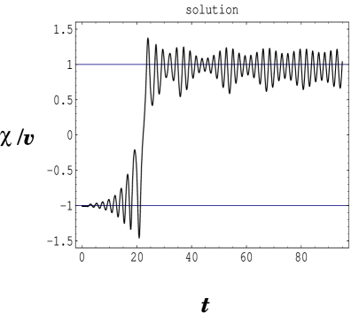
FIG. 3.: Classical solution of the equation of motion in the potential of Fig. 1. The evolution begins near the unstable classical trajectory $\chi(t)=-v$ and is driven towards a stable classical solution $\chi(t)=+v$. In quantum theory, if the tunneling rate between the two vacua is small, a phase transition to a metastable vacuum takes place.

If the tunneling rate between $\langle\chi\rangle=+v$ and $\langle\chi\rangle=-v$ is negligible, the classical evolution shown in Fig. 3 describes a phase transition into a metastable false vacuum.

This example shows that the ground state at the end of inflation does not necesarily correspond to the global minimum of the potential. Instead, during the preheating, a false vacuum can be populated if the true vacuum entered in resonace while the false vacuum did not.

Both Grand Unified Theories and supersymmetric extentions of the Standard Model predict the existence of local minima in the effective potential. The tunneling rate between these minima can be extremely low and their lifetimes can easily exceed the present age of the universe. For example, the effective potential of the MSSM can have a broken color SU(3) in its global minimum, while the standard, color and charge conserving vacuum is metastable. For natural and experimentally allowed values of the MSSM parameters, the lifetime of this false vacuum can be much greater than $10^{10}$ years [7]. If the reheat temperature after inflation was not much higher than the electroweak scale, this metastable minimum could be populated in the way we have described.

Breaking a SUSY GUT gauge group and choosing between the nearly degenerate minima is problematic in non-inflationary cosmology [8]. Let us consider a SUSY SU(5) GUT for example. The minima with unbroken SU(5), SU(4)$\times$U(1), and SU(3)$\times$SU(2)$\times$U(1) groups are nearly degenerate, split only by supersymmetry breaking terms of the order of a TeV. Why did the universe end up in the vacuum with the lowest symmetry?

Finite temperature corrections (if relevant, which may not be the case for preheating) make the SU(5) minimum lowest in energy because it has a higher number of degres of freedom. The subsequent thermal evolution of the potential makes tunneling into a Standard Model vacuum impossible [8] even if it becomes the global minimum at temperatures below 1 TeV. Supergravity splits the three minima by a negligible amount and in such a way that cosmological constant can by fine-tuned to zero only in the minimum with the higher energy while the other two minima have negative energy density [9]. Some of the proposed solutions [8] rely on assumptions about a strong gauge dynamics that seem somewhat implausible.

If, however, inflation took place, the SUSY GUT vacuum could be chosen in a phase transition of the kind we described. This appears to resolve a long-standing problem concerning the breaking of the SUSY GUT gauge group.

III B+L violation

As discussed in the Introduction, preheating oscillations of the Higgs VEV can lead to two effects of interest for B+L violation. The first [6] is that the sphaleron barrier itself oscillates, leading in principle to exponentially-sensitive oscillations of the sphaleron rate. The second, which we take up here, is that Higgs oscillations can resonantly drive classical transitions over the barrier.

Given an appropriate CP-violating seed, there are three stages to this classical resonant driving. In the first stage, the seed (which can be a source term or initial conditions on the EW gauge potentials) drives large-scale generation of Chern-Simons (CS) number (topological charge) over spatial scales so large that spatial variation can be ignored and only temporal variation saved in the classical equations of motion. In the second stage, gradients on shorter scales emerge, as a result of unstable growth of spatially-dependent perturbations. The seeds for these spatial modes might emerge from spinodal decomposition during inflation [10, 11]. As expected on general grounds from earlier preheating studies, the fastest-growing modes are those with large spatial scales. The third stage involves the generation of sphalerons, with spatial scales at the standard W-boson mass $M_{W}$.

In all stages, we will ignore various back-reaction effects; the expansion of the universe (in any case, neglible for weak-scale inflation); and damping produced by perturbative decays (one order of $\alpha_{W}$ higher than terms we keep).

We discuss the first stage, which has important non-linear effects stemming from gauge-potential self-coupulings, both analytically and numerically. A particular ansatz is used for the gauge potential, having only a time dependence. (This ansatz has been used some time ago [12] in a rather different scenario.) The analysis is in the same spirit as the conventional approach to low-order resonances in the Mathieu equation (see, e.g., Ref. [13]). But the lowest-order resonant-mode equations, two first-order differential equations, have a cubic non-linearity. Surprisingly, these coupled non-linear equations can be solved exactly in terms of elliptic functions. The non-linear terms not only provide a quartic potential opposing the growth of CS number but, as the CS number grows, the non-linear term also grows and drives the system off resonance. In effect, the cubic non-linearity causes the W-boson mass to increase. Interestingly, this increase can be offset by a secular increase of the frequency of Higgs oscillations, allowing resonance to be maintained for long periods of time with consequent large growth of CS number.

In the second stage we include linear perturbations to the spatially-homogeneous equations of the first stage; these perturbations are considered to lowest order in spatial gradients, as characterized by a spatial momentum $k$. It is not possible to do a conventional dispersion-relation analysis of these equations, which have time-dependent coefficients as determined by the temporal growth of the first-stage gauge potentials. We perform a numerical analysis of the three coupled linear differential equations which result.

The third stage, in which gradients evolve to spatial scales $\sim M_{W}^{-1}$ appropriate for sphalerons, is the hardest to analyze, since an adequate treatment involves the solution of coupled partial differential equations with time-dependent coefficients. So we restrict ourselves to a crude, simple first step, reducing these partial differential equations by a non-linear ordinary differential equation for an approximate sphaleron-like mode. The relevant gauge-potential ansatz, first introduced by Bitar and Chang [14], was later used [15] to analyze sphalerons above the EW phase transition, and was shown to have an effective barrier potential for the sphaleron which was numerically very close to that of a simple pendulum. We introduce an oscillating Higgs field, which causes this pendulum to be parametrically-driven. The ansatz is too simple to be used for anything more than estimating the rate of change of topological charge as the pendulum goes over its barrier once; we do this numerically. In principle, more complicated forms, representing multiple sphalerons, could be used, such as the ADHM construction or those of ’t Hooft or of Jackiw, Nohl, and Rebbi [16] multi-instanton form, suitably modified for Minkowski-space dynamics, but these have not yielded any insights for us.

At all stages, the energy density associated with generation of CS number is of order $4\pi m^{4}/g^{2}$, as would be appropriate for a gas of sphalerons with density $\sim m^{3}$.

A First stage: homogeneous CS parametric resonance

In what follows we always consider the Higgs field to have a given VEV, as determined by preheating effects. Introduce the conventional anti-hermitean gauge potential, with coupling $g$ included, by:

$$gA_{\mu}=(\frac{\tau_{a}}{2i})A_{\mu}^{a}.$$ (2)

Our spatially-homogeneous ansatz is:

$$gA_{0}=0;\;gA_{i}=(\frac{\tau_{i}}{2i})\phi(t)$$ (3)

in which the group index is tied to the spatial index. By the conventional rules of charge conjugation and parity for the gauge potential, $\phi$ is C even, P odd, CP odd.

It is important to note that this ansatz does not correspond to a non-vanishing VEV for an EW field. Gauge invariance alone is enough to ensure that there can be no expectation value coupling the space-time indices to group indices.

One readily calculates the EW electric and magnetic fields:

$$gE_{i}\equiv G_{0i}=(\frac{\tau_{i}}{2i})\dot{\phi}(t);\;gB_{i}\equiv\frac{1}{2}\epsilon_{ijk}G_{jk}=(\frac{\tau_{i}}{2i})\phi^{2}.$$ (4)

Then one calculates the density $W$ of Chern-Simons number as:

$$W=(\frac{1}{8\pi^{2}})\phi^{3}.$$ (5)

It is straightforward to check that $\dot{W}$ is the topological charge density $Q$, related to B+L violation through the anomaly equation.

With the assumption of a given Higgs VEV, the equations of motion for the gauge potential are:

$$[D^{\mu},G_{\mu\nu}]+M_{W}^{2}(t)(A_{\nu}+(\partial_{\nu}U)U^{-1})=0.$$ (6)

Here the unitary matrix $U$ represents the Goldstone (phase) part of the Higgs field. The mass term will be assumed to have the form:

$$M_{W}^{2}(t)=m^{2}(1+\epsilon\cos(\omega t))$$ (7)

where $m$ is the value of $M_{W}$ with no oscillations. Later we will have occasion to consider a time-dependent frequency $\omega$, but for now think of it as a constant.

There must be some sort of CP-violating seed to produce non-zero solutions of the equations of motion; these might stem from (long-scale) spatial gradients in the matrix $U$, which acts as a source in equation (6), or from initial values of $\phi$. Because the equations are unstable, there is little practical difference, and we choose to drop the $U$ terms in the equations of motion, and then providing a seed through initial values. Then there is a single equation for $\phi$:

$$\ddot{\phi}+2\phi^{3}+(1+\epsilon\cos rt)\phi=0$$ (8)

We have non-dimensionalized the equations of motion by measuring $\phi$ in units of $m$ and time $t$ in units of $m^{-1}$. The parameter $\rho$ has the value $\omega/m$.

Without the cubic non-linearity, this would be a standard Mathieu equation. In the Appendix we analyze the coupled non-linear mode equations which arise for the lowest resonance ($r=2$), and find that they can be solved exactly in terms of elliptic integrals. The qualitative features of this analysis are easy to anticipate: Equation (8) describes the motion of a particle in a quartic potential. The oscillating term drives the particle up the wall, but eventually the particle gets out of resonance and falls back. This process can repeat quasi-periodically.

FIG. 4.: Time dependence of $\phi$ for initial values as in equation (9) plus $r=2.3,\epsilon=0.9$.

We now turn to numerical analysis. Only a couple of examples will be reported, without attempting to choose parameters to correspond to realistic preheating scenarios. Parameters are chosen to illustrate specific effects; other parameter sets may show no interesting behavior at all. The runs reported here have initial values

$$\phi(0)=0.001;\;\dot{\phi}(0)=0,$$ (9)

and large values of $\epsilon$, in the range 0.5-0.9. Because the equations are both non-linear and unstable, the final results are largely independent of the initial conditions as long as they are non-zero. As the initial values are reduced, the time of onset of instability is sometimes lengthened. Generally, there are two regimes (for constant frequency $\omega$): The resonant regime, in which $\phi$ grows to O(1), and the non-resonant regime where $\phi$ stays small. We will only show the near-resonant cases in the figures. There is another regime in which $\omega$ grows secularly with time, and which leads to larger values of $\phi$.

Fig. 4 is a typical example of the behavior when $\omega$ or $r$ is constant and fairly near resonance (in this case, $r$=2.3). One sees that the envelop of $|\phi|$ grows to order unity, but periodically passes through zero and repeats. This is because $\epsilon$ is near unity, and so system frequencies vary quite a bit, from $1+\epsilon$ to $1-\epsilon$.

Fig. 5 shows the behavior when the frequency grows secularly. The onset of rapid growth is delayed because the system is originally fairly far from resonance, but then the envelop of $|\phi|$ grows essentially linearly, coupled to the frequency change. The system is able to stay in resonance as $\phi$ grows linearly, because the effective mass $M$ of the $\phi$ field (see the Appendix) is $M^{2}\simeq m^{2}+3\langle\phi^{2}\rangle$, and the effective ratio $r=\omega/M$ stays roughly constant if $M$ grows at the same rate as $\omega$.

Fig. 6 shows the CS density $\phi^{3}/8\pi^{2}$ corresponding to the parameters of Fig. 5. The CS density grows roughly as $t^{3}$, with $\phi$ growing linearly in time as does $\omega$.

With dimensionalized values of $|\phi|\simeq m$, the CS number density is of order 0.01 $m^{3}$, corresponding to a large B+L density. Whether any of this CS density survives preheating to the reheating phase depends on whether there is a “graceful exit” to preheating generation of CS number, and this depends on factors not considered in this paper, such as back reaction, growth of finite-momentum modes, and linear damping by decay of the W-boson condensate. Additionally, there may be many domains large compared to $m^{-1}$ but small compared to the Hubble size in which the values of $\phi$ are uncorrelated. This will reduce the effective global CS density by a factor of $N^{1/2}$, where $N$ is the number of such domains. The ultimate fate of the processes considered here will be taken up in a future work, in which specific weak-scale preheating scenarios will be taken up.

FIG. 5.: Behavior of $\phi$ with the initial conditions of equation (9), with $b=0.52$, and a secularly-growing frequency $r(t)=1.7+0.001t$.

FIG. 6.: The Chern-Simons density (see equation (5)) for the parameters of Fig. 5.

B Second stage: evolution of spatially-varying modes

Ultimately, there will be some CP-violating seeds with finite spatial gradients. Assuming that these seeds are smaller than those for $\phi$ (as is reasonable following inflation), these seeds will be driven by the time variation of $\phi$ as well as of the Higgs VEV. We will be concerned here only with the linearized equations for the spatially-varying modes, which we characterize in momentum space. As is usual in preheating phenomena, the modes with the longest spatial scales (smallest $k$) grow fastest.

The total vector potential is written as $A_{\mu}+a_{\mu}$, with $A_{\mu}$ taken from equation (3). The most general vector potential $ga_{\mu}$ depending on a single vector $\vec{k}$ has time component

$$ga_{0}=(\frac{i\vec{\tau}\cdot\hat{k}}{2i})\alpha_{0},$$ (10)

and space components

$$ga_{j}=\frac{1}{2i}[(\tau_{j}-\hat{k}_{j}\vec{\tau}\cdot\hat{k})\beta_{1}+i\epsilon_{jab}\tau_{a}\hat{k}_{b}\beta_{2}+\hat{k}_{j}\vec{\tau}\cdot\hat{k}\beta_{3}].$$ (11)

In equations (10,11) the hat indicates a unit vector, and $\alpha_{0},\beta_{i}$ are real functions of $k^{2}$ and $t$. As before, we non-dimensionalize by dividing these functions by $m$, replacing $t$ by $mt$, and $k$ by $k/m$. Presumably the Fourier transforms in (10,11) vanish at an appropriate rate as $k\rightarrow 0$ so as to change $\hat{k}$ into $\vec{k}$, although this will not matter in what follows.

It is straightforward if lengthy to write out the linearized version of equation (6) (without the $U$ terms):

$$\alpha_{0} = \frac{1}{Q}[2(\dot{\phi}\beta_{2}-\dot{\beta}_{2}\phi)-k\dot{\beta}_{3}],$$ (12)

$$Q = k^{2}+2\phi^{2}+1+\epsilon\cos rt;$$ (13)

$$\ddot{\beta}_{1}+Q\beta_{1}-2k\phi\beta_{2}+2(\beta_{1}+\beta_{3})\phi^{2}=0;$$ (14)

$$\ddot{\beta}_{2}+Q\beta_{2}-2k\phi\beta_{1}+\phi(\dot{\alpha}_{0}-k\beta_{3})+2\dot{\phi}\alpha_{0}=0;$$ (15)

$$\ddot{\beta}_{3}+Q\beta_{3}+k(\dot{\alpha}_{0}-k\beta_{3}-2\phi\beta_{2})+4\beta_{1}\phi^{2}=0.$$ (16)

Even though these are linear equations for the modes $\alpha_{0},\beta_{j}$ they are impossible to solve analytically, because $\phi$ is not an analytically-known function. We have solved them numerically, with various interesting results. Perhaps the most interesting is that these mode functions remain small and well-behaved for a long time, and then when $\phi$ is large enough (of order unity) they show violently unstable behavior. This is especially so for the case when the frequency $\omega$ is growing with time, as for Fig. 5. This is illustrated in Fig. 7, showing the evolution with time of the linear modes for the parameters of Fig. 5. The mode functions were begun with initial values which are 0.1 times those of $\phi$ (see equation (9)). Of course, any other initial values can be gotten by scaling, since the equations are linear. The point is that when, for a given set of initial values of $\alpha_{0},\beta_{j}$, these functions rise to be of O(1), the whole problem becomes non-linear and presumably enters something like the third stage discussed below. Note in Fig. 7 that the threshhold for non-linearity, with the given initial conditions, occurs at a (dimensionless) time of 200, which gives $\phi$ enough time to get big enough to be interesting (see Fig. 5).

FIG. 7.: The evolution of the linear modes for the parameters of Fig. 5. Note the truncation on the vertical axis; at $t\simeq$ 200

all the amplitudes are larger than one in magnitude.

C Third stage: sphalerons

Eventually, momentum modes with $k\simeq 1$ will become prominent, and the condensate of CS number becomes a condensate of sphalerons. It is much more difficult to describe this stage, and we will only take a simple first step. This step consists of a drastic simplification of the kinematics of a sphaleron coupled to a time-dependent Higgs field, reducing the dynamics to a single function $\lambda(t)$ as in Refs. [14, 15]. Write the most general spherically-symmetric gauge potential and Higgs phase matrix $U$ in the form:

$$U=\exp[\frac{i\gamma}{2}\hat{r}\cdot\vec{\tau}],\;gA_{0}=\frac{1}{2i}\hat{r}\cdot\vec{\tau}H_{2};$$ (17)

$$gA_{i}=\frac{1}{2ir}[\epsilon_{iak}\tau_{a}\hat{r}_{k}(\phi_{1}-1)-(\tau_{i}-\hat{r}_{i}\hat{r}\cdot\vec{\tau})\phi_{2}+\vec{r}_{i}\hat{r}\cdot\vec{\tau}H_{1}.$$ (18)

The functions $H_{i},\phi_{j}$ depend only on $r,t$. The asymptotic values of the angle $\gamma$ are zero at $r=0$ and $\pi$ at $r=\infty$. We parametrize these functions as:

$$H_{1} = \frac{2\lambda}{\lambda^{2}+r^{2}+a^{2}};$$ (19)

$$H_{2} = -\frac{2r\dot{\lambda}}{\lambda^{2}+r^{2}+a^{2}};$$ (20)

$$\phi_{1} = 1-\frac{2r^{2}}{\lambda^{2}+r^{2}+a^{2}};$$ (21)

$$\phi_{2} = -\frac{2r\lambda}{\lambda^{2}+r^{2}+a^{2}}.$$ (22)

For details on the parametrization of $\gamma$ see [15]. For the present purpose one can just think of $\gamma$ as always equal to $\pi$. In this parametrization the constant $a$ is a size parameter (like that of an instanton) and $\lambda$, the sole dynamic degree of freedom, depends on $t$. Generally, $\lambda$ is an odd function of $t$, vanishing along with its first derivative at $t=0$.

The electric and magnetic fields are:

$$gE_{j} = (\frac{\tau_{j}}{2i})\frac{4a^{2}\dot{\lambda}}{\lambda^{2}+r^{2}+a^{2}};$$ (23)

$$gB_{j} = (\frac{\tau_{j}}{2i})\frac{4a^{2}}{\lambda^{2}+r^{2}+a^{2}}.$$ (24)

Note that these have the same space and internal symmetry index dependence as does the $\phi$ ansatz of equation (3). It is therefore natural to suppose that the $\phi$ fields will transform (through the growth of spatial modes) into a condensate of sphalerons. Of course, in this condensate each sphaleron will be a translate in space and in time of the sphaleron exhibited here, which is centered at the space-time origin.

With boundary conditions

$$\lambda(t=-\infty)=-\infty;\;\lambda(t=+\infty)=+\infty$$ (25)

one readily verifies that, no matter what the dynamics of $\lambda$ as long as it is single-valued, the (Minkowskian) topological charge

$$Q=-\frac{g^{2}}{4\pi^{2}}\int d^{4}xTr\vec{E}\cdot\vec{B}$$ (26)

has the value 1. Indeed, if we replace $\lambda$ by $t$ we get exactly the usual Euclidean one-instanton expression, which however is now being interpreted as a Minkowskian construct.

The size coordinate $a$ is not arbitrary, as it is for instantons in gauge theories with no Higgs field. As shown in [15], if one goes to $t=0$ and sets $\lambda,\dot{\lambda}=0$ there, the resulting $ansatz$ in equations (16,17) is an excellent trial wave function for the sphaleron. Minimizing the Hamiltonian (for time-independent Higgs VEV) yields $a=\sqrt{3}/2M_{W})$ and a sphaleron mass $M_{s}$ only a fraction of a percent higher than the true value, determined numerically, of

$$M_{s}=5.41(\frac{4\pi M_{W}}{g^{2}}).$$ (27)

When the mass $M_{W}$ depends on time, as in equation (7), we will continue to use the above value for $a$. It then happens that the parameters of the Hamiltonian depend on time (see [15] for the Hamiltonian as a function of $a,\lambda,\dot{\lambda}$).

As is further shown in [15], one can trade the function $\lambda$ for a topological charge $Q(t)$ defined by demanding that the kinetic energy term in the Hamiltonian is of the form $(1/2)I\dot{Q}^{2}$ with $I$ independent of $Q$. The normalization

$$\lambda=-\infty:\;Q=0;\;\lambda=+\infty:\;Q=2\pi$$ (28)

makes the topological charge an angular variable. Numerical work shows that the potential energy is very nearly that of a pendulum, and that $I=\xi M_{s}/m^{2}$ for some numerical constant $\xi$. The resulting approximate Hamiltonian has the form:

$$H=M_{s}[\frac{\xi}{2M_{W}^{2}}\dot{Q}^{2}-\cos Q]$$ (29)

which has, as it must, the value $M_{s}$ when $\dot{Q}=0,\;Q=\pi$.

Next one replaces $M_{W}$ by its time-dependent value, as in equation (7). We have numerically investigated such driven pendulum equations. They lead to multiple transitions over the barrier, but we will not display such solutions here. One reason is that the ansatz we use here is strictly tied to a unit change of topological charge, so that all that counts is the rate of making a single transition over the barrier. Just as for all the classical barrier-hopping solutions presented for the $\phi$ ansatz, the rate is $O(\omega)$, very much different from the tunneling rate. (The tunneling rate is also changed as the sphaleron mass oscillates; see [6].)

To go further than this for a condensate of real sphalerons is extraordinarily complicated; each sphaleron, like the instanton to which it corresponds, has numerous degrees of freedom. Even if we restrict this to one degree of freedom (corresponding to $\lambda$) for each sphaleron, it is not clear how to proceed. Nor is it clear how to modify known multi-instanton ansätze such as ADHM or that of ’t Hooft or Jackiw, Nohl, and Rebbi [16] to express the real-time sphaleron dynamics in the presence of an oscillating Higgs field.

IV Conclusions

In this work we have investigated two new mechanisms driven by preheating oscillations of, e.g., the Higgs field in hybrid inflation. The first mechanism, resonant barrier-crossing from a lower minimum to a higher minimum (where there is no longer resonance), may explain some puzzles associated with the symmetry-breaking patterns of GUTs. This kind of transition could also populate a metastable SU(3)$\times$SU(2)$\times$U(1) vacuum in a supersymmetric extension of the Standard Model even if the global minimum of the potential breaks charge and color. (In the case of the MSSM, this posibility has direct inplications for collider experiments [7].) The second mechanism, resonant barrier-crossing associated with B+L violation, may lead to a condensate of sphalerons on time scales short compared to tunneling rates. Both effects require resonance with preheating oscillations to be effective. We have not tried to construct “realistic” applications of these mechanisms to specific preheating scenarios. We note, however, that in many cosmological models, even if the initial conditions are far from resonance, the system evolves and reaches the resonance eventually, thanks to a change in the relevant parameters [1]. Such evolution is facilitated by either non-quadratic inflaton potential that causes a variation in the inflaton frquency, of by expansion of the universe and the associated Hubble damping (for GUT, not weak-scale preheating), or some other effects that can slowly drive a system into a resonance band. We leave the building of realistic cosmological models for future work.

Aside from such applications, there is still a good deal of work to be done to clarify these mechanisms. In the case of B+L violation, one can raise the following issues:

1. How do the three stages (spatially-homogeneous potential, linear momentum-mode perturbations, sphaleron condensate) of Section III evolve from the first to the last? This can only be answered by numerical work more extensive than we have yet done.

2. The large-scale EW CS density we propose will have a projection onto Maxwell magnetic fields carrying helicity (another term for Chern-Simons number). The spatially-homogeneous nature of these fields makes them quite different from earlier proposals (see [17, 18] and references therein) involving generation of Maxwell fields in a thermal environment, with unacceptably small scale lengths to correspond to the scale lengths of present-day galactic magnetic fields. Given sufficient inverse cascading of the nearly-homogeneous Maxwell fields following from our preheating mechanism (at EW time these fields must be limited in extent by the Hubble size), [18] shows that EW-time Maxwell fields could indeed be the seeds for presently-observed galactic fields. We intend to investigate this further.

3. Can one make use of multi-instanton ansätze such as those of ADHM, ’t Hooft, or Jackiw, Nohl, and Rebbi [16] to extend the Bitar-Chang [14] construction we have exploited in Section IIIC in order to understand quasi-analytically the formation of a sphaleron condensate?

4. Are there (necessarily spin-dependent) quasi-resonant phenomena for the production of W-bosons by an oscillating Higgs field which are in any sense analogous to the very sharp resonant phenomena found by Cornwall and Tiktopoulos [19] for spin-1/2 charged particles in specific time-dependent electric fields?

To clarify this last point, Ref. [19] found that it is possible to have highly-resonant $e^{+}e^{-}$ pair production in a classical time-varying electric field of the proper time dependence. The sharply-resonant nature of the process can only happen for fermions, but in any case spin effects, which might be available with gauge bosons, are important in overcoming the typical $\exp(-1/\alpha)$ rate of pair production in classical fields.

Analysis of mode equations for $\phi$

Here we give the analysis of the Mathieu-like but non-linear modal equations of Section III. Just as for the Mathieu equation, we write the non-dimensionalized $\phi$ in the form

$$\phi=a(t)\cos(rt/2)+b(t)\sin(rt/2),$$ (30)

(where, as in the main text, $r=\omega/m$), leaving out all terms with higher frequencies. One verifies that the time dependence of $a,b$ is $O(\epsilon)$, so that we can ignore second derivatives of these quantities. However, we will save the cubic non-linearities.

Using equation (A1) in the equation of motion (8), saving only terms varying as $\cos(rt/2)$ and $\sin(rt/2)$, and dropping second derivatives yields:

$$r\dot{a}+b[\frac{r^{2}}{4}+\frac{1}{2}\epsilon-1-\frac{3}{2}(a^{2}+b^{2})]=0;$$ (31)

$$-r\dot{b}+a[\frac{r^{2}}{4}-\frac{1}{2}\epsilon-1-\frac{3}{2}(a^{2}+b^{2})]=0.$$ (32)

To make contact with the linear Mathieu equation, let us temporarily replace the terms $(3/2)(a^{2}+b^{2})$ by constants, and define an effective (non-dimensional, that is, scaled by $m$) mass $M$ by:

$$M^{2}\equiv 1+\frac{3}{2}(a^{2}+b^{2}).$$ (33)

Assuming exponential growth, with $a,b\sim\exp(\mu t)$, gives:

$$mu=\frac{1}{2r}[\epsilon^{2}-(r^{2}-4M^{2})^{2}]^{1/2}$$ (34)

which gives growth only when $r=2M+O(\epsilon)$. For small initial values of $\phi$ this means $r\simeq 2$, but as $\phi$ grows because of the initial parametric resonance, the system goes out of resonance.

We show that equations (A2,A3) can be solved exactly in terms of elliptic integrals. Multiply (A2) by $a$ and (A3) by $-b$ and add to get:

$$\frac{d}{dt}(a^{2}+b^{2})=-(\frac{2\epsilon}{r})ab.$$ (35)

This equation is independent of the non-linear terms in (A2,A3); it would hold even if these terms were dropped. Note that exponential growth requires $a,b$ to be of opposite sign. The constraints expressed by equation (A6) allow the elimination of one degree of freedom:

$$a=A\cos\Psi,\;\;b=-A\sin\Psi,$$ (36)

with a relation between $A$ and $\Psi$:

$$A=A_{0}\exp\int_{0}^{t}dt^{\prime}(\frac{\epsilon}{2r})\sin 2\Psi(t^{\prime})$$ (37)

with $A_{0}$ as an initial value. In the linear (Mathieu) case $\cos\Psi$ is the constant $|r^{2}-4|/\epsilon$, which yields the linear growth rate in equation (A5). But equations (A2,A3) yield two equations for the time evolution of $A<\Psi$. The sum of these equations is a trivial identity, while the difference (using equations (A7,A8)) is:

$$\epsilon\cos 2\Psi-2r\dot{\Psi}=\frac{r^{2}}{2}-2-3A_{0}^{2}\exp\int_{0}^{t}dt^{\prime}(\frac{\epsilon}{2r})\sin 2\Psi(t^{\prime}).$$ (38)

Now differentiate (A9) and use (A9) in the result to arrive at:

$$2\ddot{\Psi}-\frac{\epsilon}{2r^{2}}(r^{2}-4)\sin 2\Psi+\frac{\epsilon^{2}}{2r^{2}}\sin 4\Psi.$$ (39)

This is readily checked to be an elliptic equation. We will not bother to study it here. All the physics is contained in the linearization of (A10), which gives:

$$\Psi(t)=\Psi_{0}\cos[(\lambda(t-t_{0})]$$ (40)

with frequency

$$\lambda=[\frac{\epsilon^{2}}{r^{2}}-\frac{\epsilon(r^{2}-4)}{2r^{2}}]^{1/2}.$$ (41)

Since $r^{2}-4$ is $O(\epsilon)$, so is $\lambda$. The best case for growth is

$$\Psi(t)=(\frac{\pi}{4})\cos\lambda t$$ (42)

(so that $A$ and $b$ are equal initially). Evidently, from (A8) growth stops when $\Psi=0$, or when $t=\pi/2\lambda$. This means, as discussed in the main text, that growth cannot be unlimited. (However, when the frequency $r$ grows secularly, growth can continue unimpeded with $a^{2},b^{2}\sim r$, which maintains the resonant growth condition.) Generally, no matter how small the initial values of the potential $\phi$, eventually $\phi$ becomes of order unity. The smaller the initial value, the longer this process takes.

REFERENCES

- [1] L. Kofman, A. Linde and A. A. Starobinsky, Phys. Rev. Lett. 73, 3195 (1994); Phys. Rev. D 56, 3258 (1997).
- [2] L. Kofman, A. Linde and A. A. Starobinsky, Phys. Rev. Lett. 76, 1011 (1996) [hep-th/9510119]; I. I. Tkachev, Phys. Lett. B376, 35 (1996) [hep-th/9510146]; S. Khlebnikov, L. Kofman, A. Linde and I. Tkachev, Phys. Rev. Lett. 81, 2012 (1998) [hep-ph/9804425].
- [3] G. W. Anderson, A. Linde and A. Riotto, Phys. Rev. Lett. 77, 3716 (1996) [hep-ph/9606416]; E. W. Kolb, A. Linde and A. Riotto, Phys. Rev. Lett. 77, 4290 (1996) [hep-ph/9606260]; E. W. Kolb, A. Riotto and I. I. Tkachev, Phys. Lett. B423, 348 (1998) [hep-ph/9801306].
- [4] L. M. Krauss and M. Trodden, Phys. Rev. Lett. 83, 1502 (1999) [hep-ph/9902420].
- [5] J. Garcia-Bellido, D. Grigorev, A. Kusenko and M. Shaposhnikov, Phys. Rev. D60, 123504 (1999) [hep-ph/9902449].
- [6] J. Garcia-Bellido and D. Grigoriev, hep-ph/9912515.
- [7] M. Claudson, L. J. Hall and I. Hinchliffe, Nucl. Phys. B228, 501 (1983); A. Riotto and E. Roulet, Phys. Lett. B377, 60 (1996) [hep-ph/9512401]; A. Kusenko, P. Langacker and G. Segre, Phys. Rev. D54, 5824 (1996) [hep-ph/9602414]; A. Riotto, E. Roulet and I. Vilja, Phys. Lett. B390, 73 (1997) [hep-ph/9607403]; A. Kusenko and P. Langacker, Phys. Lett. B391, 29 (1997) [hep-ph/9608340].
- [8] For review, see, e.g., H. P. Nilles, Phys. Rept. 110 (1984) 1.
- [9] S. Weinberg, Phys. Rev. Lett. 48 (1982) 1776.
- [10] D. Cormier and R. Holman, hep-ph/9912483.
- [11] S. Tsujikawa and T. Torii, hep-ph/9912499.
- [12] J. M. Cornwall, Phys. Lett. B243, 271 (1990).
- [13] L. D. Landau and E. M. Lifshitz, Mechanics, third edition (Pergamon Press, Oxford, 1969), p. 80.
- [14] K. M. Bitar and S. Chang, Phys. Rev. D17, 486 (1978).
- [15] J. M. Cornwall, Phys. Rev. D40, 4130 (1989).
- [16] R. Jackiw, C. Nohl and C. Rebbi, Phys. Rev. D15, 1642 (1977).
- [17] J. M. Cornwall, Phys. Rev. D56, 6146 (1997) [hep-th/9704022].
- [18] G. B. Field and S. M. Carroll, astro-ph/9811206.
- [19] J. M. Cornwall and G. Tiktopoulos, Phys. Rev. D39, 334 (1989).