RHEINISCH WESTFÄLISCHE TECHNISCHE HOCHSCHULE AACHEN PITHA 98/44
 
Dezember 1998

Power Corrections to

Event Shape Variables

measured in

ep Deep-Inelastic Scattering
Klaus Rabbertz

I. Physikalisches Institut der Technischen Hochschule Aachen

 

PHYSIKALISCHE INSTITUTE
RWTH AACHEN
52056 AACHEN, GERMANY

Power Corrections to
Event Shape Variables
measured in
$ep$ Deep-Inelastic Scattering
Von der Mathematisch-Naturwissenschaftlichen Fakultät

der Rheinisch-Westfälischen Technischen Hochschule Aachen

genehmigte Dissertation zur Erlangung des akademischen Grades

eines Doktors der Naturwissenschaften

vorgelegt von

Diplom-Physiker
Klaus Rabbertz
aus Mönchengladbach

Berichter	:	Universitätsprofessor Dr. Ch. Berger
	:	Universitätsprofessor Dr. S. Bethke
Tag der mündlichen Prüfung	:	23.12.1998

Meinen Eltern

Ceci n’est pas une pipe.—René Magritte

Abstract

Deep-inelastic $ep$ scattering data, taken with the H1 detector at HERA, are used to study event shape variables over a large range of “relevant energy” $Q$ between $7\,{\rm GeV}$ and $100\,{\rm GeV}$. Previously published analyses on thrust, jet broadening, jet mass and $C$ parameter are substantially refined and updated; differential two-jet rates treated as event shapes are presented for the first time.

The $Q$ dependence of the mean values is fit to second order calculations of perturbative QCD applying power law corrections proportional to $1/Q^{p}$ to account for hadronization effects. The concept of these power corrections is tested by a systematic investigation in terms of a non-perturbative parameter $\overline{\alpha}_{p-1}$ and the strong coupling constant.

Kurzfassung

Ereignisformvariablen in der tiefinelastischen $ep$-Streuung, gewonnen aus Daten des H1-Detektors bei HERA, werden über einen großen Bereich der „relevanten Energieskala“ $Q$ von $7\,{\rm GeV}$ bis $100\,{\rm GeV}$ untersucht. Bereits publizierte Studien zu thrust, Jetbreite, Jetmasse und $C$ Parameter werden erheblich verbessert und aktualisiert; Ergebnisse zu differentiellen Zweijetraten als Ereignisformen werden erstmals vorgestellt.

Bei der Anpassung der $Q$-Abhängigkeit der Mittelwerte an Berechnungen der perturbativen QCD in zweiter Ordnung sollen potenzartige Korrekturterme der Form $1/Q^{p}$ Hadronisierungseffekte berücksichtigen. Eine Überprüfung des Konzepts solcher Potenzkorrekturen erfolgt im Rahmen der Bestimmung eines nichtperturbativen Parameters $\overline{\alpha}_{p-1}$ und der Kopplungskonstanten der starken Wechselwirkung.

Kapitel 1 Introduction

Curiosity is one of mankind’s elementary driving forces — the more so when scientists are concerned. In European history the appearance of the first “professional scientists” is usually dated back to antique Greece, where, besides others, philosophers laid the foundations for a great part of European culture. Two of them living around 500 B.C., Leukippos and Demokritos, suggested first that matter consists of tiny indivisible particles called atoms. They may be considered the forefathers of today’s elementary particle physicists.

Their reasoning was of a basically theoretical nature. Turning to experiment, a “quantum leap” leads us to Antoni van Leeuwenhoek (1632–1723). Employing microscopes he constructed himself, he was able to observe “creatures that swarm and multiply in a drop of water” for the first time.

With the advent of the modern microscope Hadron-Elektron-Ring-Anlage HERA at the Deutsches Elektronen-SYnchrotron DESY in Hamburg three centuries later, the resolution power could be increased by about twelve orders of magnitude. Now it is possible to study “gluons that propagate and split in a droplet of nuclear matter called proton.”

The theory that is believed to describe the strong interaction, responsible for the structure of hadronic (nuclear) matter, is called Quantum ChromoDynamics (QCD) in analogy to Quantum ElectroDynamics (QED) dealing with the electromagnetic interaction. Both are part of a more comprehensive theory usually referred to as the Standard Model (for introductory textbooks s. e.g. [1, 2, 3, 4]). It unites three, the weak, electromagnetic and strong interaction, out of the four fundamental forces observed in nature into a common framework. Gravity so far does not fit in. Comprising merely twelve elementary particles of spin $1/2$, six quarks and six leptons, and the spin $1$ exchange quanta of the three forces, i.e. the $Z^{0}$ and $W^{\pm}$ bosons, the photon $\gamma$ and eight gluons $g$, the Standard Model gives a very good account of a tremendous amount of data gathered by experiments during the last decades [5].

The HERA collider offers the unique possibility to investigate the structure of the proton and its interacting constituents in a completely new kinematic domain unreached by fixed-target experiments. With respect to this analysis, the large accessible range in “relevant energy” $Q$ is of great advantage. Observables can that way be studied and compared to theory in dependence of the available energy $Q$ in a single experiment. To that goal, the thesis is organized as follows:

Chapter two describes the machinery necessary to perform $ep$ scattering experiments at the required high energies with special attention to the parts relevant for this analysis. The third chapter explains the basic kinematics of the scattering process. Subsequently, the observables to measure are defined in chapter four. The series of chapters five, six and seven deals in detail with the selection of data, their comparison with simulations and the correction for detector imperfections. Fully corrected data are presented. The two following chapters eight and nine are dedicated to the derivation of the necessary theoretical input employing perturbative QCD (pQCD). Finally, experimental and theoretical results are compared and combined to test the power correction approach to hadronization effects that was initiated by Dokshitzer and Webber [6]. The last chapter presents a summary and an outlook.

Kapitel 2 HERA and H1

2.1 The Storage Ring HERA

Scattering experiments are the basic tools to investigate the elementary building blocks of matter, i.e. quarks and leptons, and the fundamental forces acting between them. Two rather straightforward set-ups are $e^{+}e^{-}$  and $p\bar{p}$ colliders. In the last decades, a lot of valuable information has been accumulated with such machines [5]. However, for the detailed study of a strongly bound, hadronic object like the proton, it is preferable to use a probe that does not itself interact strongly. Fixed-target experiments employ electrons and myons as well as neutrinos to determine the structure of nucleons. To enlarge the resolving power, it is necessary to increase the energy available in the collisions by accelerating the “targets,” i.e. a collider experiment is asked for.

The Hadron-Elektron-Ring-Anlage HERA, shown in fig. 2.1, is situated at DESY in Hamburg, Germany, and is currently the world’s only facility where electrons and protons are accelerated in two separate storage rings to final energies of $27.5\,{\rm GeV}$ and $820\,{\rm GeV}$ respectively. The resulting center of mass energy of about $300\,{\rm GeV}$ corresponds to electron beams of $50\,{\rm TeV}$ for fixed-target experiments. For a recent overview of the knowledge gained on the structure of nucleons consult e.g. [7].

Along the circumference of $6.3\,{\rm km}$ two locations, the north hall and the south hall, are assigned to the study of $ep$ scattering. The interaction regions, where during operation every $96\,{\rm ns}$ particle bunches may collide, are surrounded almost hermetically by complex detectors, H1 [8] and ZEUS [9]. They are dedicated to the task of measuring as many collision products as precisely as possible. Two other experiments, HERMES and HERA-B, are situated in the east and west halls and are committed to spin and $B$ meson physics respectively.

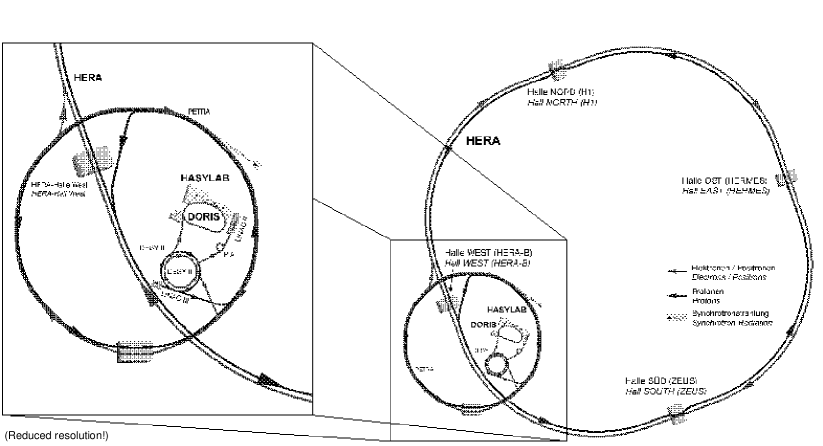
Abbildung 2.1: The storage ring HERA at the DESY laboratory in Hamburg, Germany.

2.2 The H1 Detector

The basis of this experimental analysis are data collected with the H1 detector, which is located at the northern interaction point of HERA. Only a brief overview of the total system, shown in fig. 2.2, will be given in the next section. The parts that provide the main information needed in this study will subsequently be discussed in more detail. A complete description of the detector and its performance in the first three years of operation (1992–1994) can be found in [8, 10].

During the winter shutdown 1994/95, a major upgrade of the H1 backward region was undertaken [11]. However, none of the components relevant to this analysis were significantly affected. Therefore, these improvements will not be covered here, although data from 1994 up to 1997 are used. Events where the scattered electron was found in the backward calorimeter are taken from 1994 data only.

2.2.1 Overview of the H1 Detector

The most obvious feature of the H1 detector in fig. 2.2 is its asymmetric design. Because the momentum of the protons is about $30$ times higher than that of the electrons, the $ep$ center of mass system is moving along the direction of the proton beam. As a result, the density of collision products hitting the equipment in the “forward” region is very high which is accordingly reflected in the more massive as well as finer granulated material of that part. The term “forward” refers to the conventional coordinate system used in the H1 collaboration where the proton beam direction is defined to be the $+z$-axis. The $x$-axis ($y$-axis) points from the nominal interaction point at the center of the HERA ring (upwards). Subsequently, the detector components are briefly described proceeding from the innermost parts outwards:

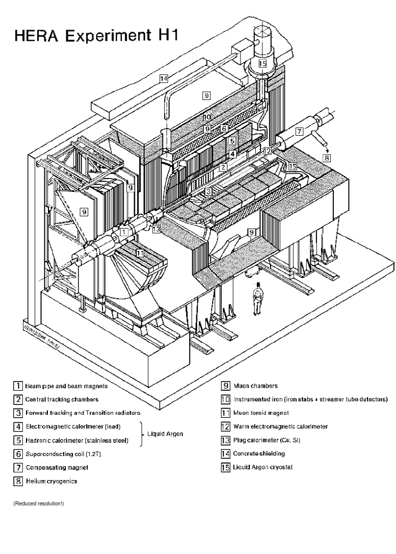
Abbildung 2.2: Schematic layout of the H1 detector.

• The tracking system:

  Directly surrounding the beam pipe and beam magnets, a tracking system is installed to measure the momentum of charged particles. It consists of two main parts: the Central Tracking Device (CTD) covering the region around the nominal interaction vertex and the Forward Tracking Device (FTD) supplementing it in the $+z$-direction.

• The calorimeters:

  To complement the momentum measurement and to detect neutral particles, the CTD and FTD are enclosed in the forward and central region by a sampling calorimeter (LAr) with Liquid Argon as active material. For the innermost absorber stacks, lead has been chosen to ensure a good containment and energy determination of electromagnetic showers produced by electrons and photons (Electromagnetic CALorimeter, ECAL). The outer part of the LAr (Hadronic CALorimeter, HCAL) predominantly measures hadronic showers and is equipped with steel absorber plates, which also serve as mechanical support structure.

  The remaining holes of the LAr around the beam pipe are closed with a silicon-copper calorimeter for polar angles below $4{{}^{\circ}}$ (PLUG) and a lead-scintillator calorimeter in the backward direction (Backward ElectroMagnetic Calorimeter, BEMC). During the upgrade in 1994/95 the BEMC was replaced by a lead-scintillating fibre Spaghetti Calorimeter (SpaCal) [12], which is subdivided into a first electromagnetic section and an additional second part to determine energy leakage and to improve the containment of hadronic showers. For the purpose of this analysis, it was only employed to supplement eventual energy deposits in the backward direction not due to the scattered electron.

• The superconducting coil:

  A cylindrical superconducting coil providing the magnetic field of $1.15\,{\rm T}$ for the trackers envelops the calorimeters. Thereby, the amount of dead material in front of the calorimeters is reduced and the time of flight of myons within the magnetic field is increased improving the resolution of their momentum measurement.

• The instrumented iron yoke and myon system:

  The IRON return yoke (IRON) of the magnet, enclosing almost completely all other parts of the detector, is sandwiched with streamer tubes for the measurement of myons and energy leakage from the inner calorimeters (Tail Catcher, TC). Supplementary chambers inside the IRON further improve the evaluation of myon tracks. Myons with high momenta in the forward direction are analyzed by a spectrometer consisting of four drift chambers in the magnetic field of $1.5\,{\rm T}$ of a toroïdal coil in front of the IRON.

• The luminosity system:

  The luminosity system sketched in fig. 2.3 utilizes the Bethe-Heitler process $ep\,\rightarrow\,ep\gamma$. The electrons and photons are detected in coincidence by a hodoscope of crystal Cherenkov counters. Whereas the electrons from these grazing collisions, i.e. $\theta_{e^{\prime}}\approx 180{{}^{\circ}}$, are deflected by magnets from the beam line to hit the Electron Tagger (ET) at $z=-33.4\,{\rm m}$, this is not possible for the photons, of course. They leave the proton beam through a window at $z=-92.3\,{\rm m}$ instead, where the beam pipe bends upwards, and reach the Photon Detector (PD) at $z=-102.9\,{\rm m}$.

  The main background is caused by bremsstrahlung from residual gas atoms $eA\,\rightarrow\,eA\gamma$. The technique of electron pilot bunches that do not have colliding proton counterparts allows to correct for it.

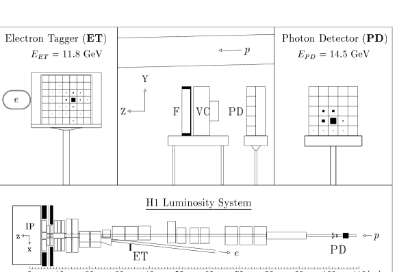
Abbildung 2.3: The layout of the H1 luminosity system [8].

2.2.2 Details on the Main Components

The basic ingredient for this analysis is the calorimetric information provided by the LAr and BEMC in the form of electromagnetic and hadronic clusters reconstructed from the primary energy depositions. The fragmentation region of the proton remnant, which is related to “soft” physics, can be excluded more easily after performing a Lorentz transformation into the Breit frame (s. section 4.1). This procedure requires a good electron identification. On the one hand, the electron cluster has to be separated from the hadronic final state, and on the other hand, it is necessary for the extraction of the event kinematics which is crucial in the calculation of the boost to the Breit frame. Therefore, additional information of the tracking system, especially the CTD, is exploited to determine the properties of the scattered electron and the actual event vertex.

The main attention in this analysis rests on mean values and normalized distributions. Hence, the luminosity system needed to measure absolute cross sections is not of prevalent importance.

Concluding, the CTD, LAr and BEMC are the most important subdetectors for the observables considered and will therefore be described in more detail [10]:

• The central tracking device CTD:

  The CTD is subdivided into two major units, the Central Jet Chambers CJC1 and CJC2 as shown in fig. 2.6 in a view perpendicular to the beam. The track reconstruction in the central region, $25{{}^{\circ}}<\theta<155{{}^{\circ}}$, depends primarily on these concentric drift chambers with wires strung parallel to the beam pipe. They provide a good space point resolution in the $(r,\phi)$-plane of $170\,{\rm\mu m}$ and, by comparing the signals at both ends, furthermore supply information about the $z$-coordinate of the hits. To avoid completely insensible paths for almost straight tracks, the sequence of the sense wires is inclined with respect to the radial direction.

  The CJC1 is sandwiched between the Central Inner and Outer Z-chambers CIZ and COZ with wires oriented in the $(r,\phi)$-plane. They complement the measurement in the CJC’s with data on the $z$-coordinate of track elements with a precision of $\approx 300\,{\rm\mu m}$.

  Mainly for the purpose of fast timing ($<96\,{\rm ns}$) and triggering, multiwire proportional chambers are added for polar angles between $5{{}^{\circ}}$ and $175{{}^{\circ}}$. Two of them, the Central Inner and Outer Proportional chambers CIP and COP, are indicated in fig. 2.6. For electrons in the backward direction, only short track segments can be seen in the CTD. The Backward Proportional Chamber BPC, consisting of four sensible layers of wires oriented along azimuthal angles of $0{{}^{\circ}}$, $45{{}^{\circ}}$, $90{{}^{\circ}}$ and $135{{}^{\circ}}$, substantially improves the tracking for polar angles of $155.5{{}^{\circ}}<\theta\leq 174.5{{}^{\circ}}$. Installed directly in front of the BEMC, fig. 2.6, it also helps to distinguish between photons and electrons in this region.

  In general, the tracking system was designed to determine the momentum and angles of charged particles to a precision of $\sigma_{p}/p^{2}\approx 0.003\,{\rm GeV}^{-1}$ and $\sigma_{\theta}\approx 1\,{\rm mrad}$.

• The liquid argon calorimeter LAr:

  As mentioned, the LAr, covering polar angles of $4{{}^{\circ}}<\theta<154{{}^{\circ}}$, is a sampling calorimeter where layers of absorber material and sensitive gaps, filled with liquid argon, alternate. Since only a sample of all energy deposits can be measured that way, the energy resolution of this technique is worse than that of calorimeters built of only one medium. To achieve nevertheless a maximal precision, care has been taken that the orientation of the absorber plates, shown in the upper part of fig. 2.6, ensures angles near the normal direction of the stacks for particles originating from the vertex. Another drawback is the difference in response on electromagnetic and hadronic showers produced by impacts of particles of the same original energy. The LAr is non-compensating.

  This is counterbalanced by stable calibration and homogeneous response properties as well as the possibility of a compact but still finely segmented construction. The structure of the read-out cells, again in an $(r,z)$-view, is presented in the lower half of fig. 2.6.

  Apart from the general subdivision in an Electromagnetic and a Hadronic section, the LAr is composed of eight wheels each further partitioned into eight octants in $\phi$. Due to the use of weak lead for the ECAL, a pointing geometry, blind for hits straight on the border between two octants, could not be avoided in contrast to the CTD. Particles reaching these $\phi$-cracks are detected only in the non-pointing HCAL. All wheels are, with respect to the nominal interaction point, combined to four aggregates: a Backward, Central and Forward Barrel and the Forward end cap with an Inner and Outer ring. The abbreviations in fig. 2.6 translate e.g. as “outer hadronic ring of forward end cap wheel 1” for OF1H.

  Test beam results yield energy resolutions of $\approx 11\%/\sqrt{E}\,\oplus\,1\%$ for electromagnetic and $\approx 50\%/\sqrt{E}\,\oplus\,2\%$ for hadronic showers. The absolute energy scales are known to $1$–$3\%$ [13] and $4\%$ for electrons and hadrons respectively.

• The backward electromagnetic calorimeter BEMC:

  A transverse view of the warm lead-scintillator calorimeter and its segmentation into $88$ stacks aligned parallel to the beam pipe can be seen in fig. 2.6. The stacks are multi-layer sandwich structures with active sampling units made of plastic scintillators. The front face directly behind the BPC is located at $z=-144\,{\rm cm}$. The angular region covered extends from polar angles of $151{{}^{\circ}}$ up to $176{{}^{\circ}}$.

  The electromagnetic energy resolution was derived from test beam measurements to be $\approx 10\%/\sqrt{E}\,\oplus\,1.7\%$, the absolute energy scale is known to a precision of $1\%$.

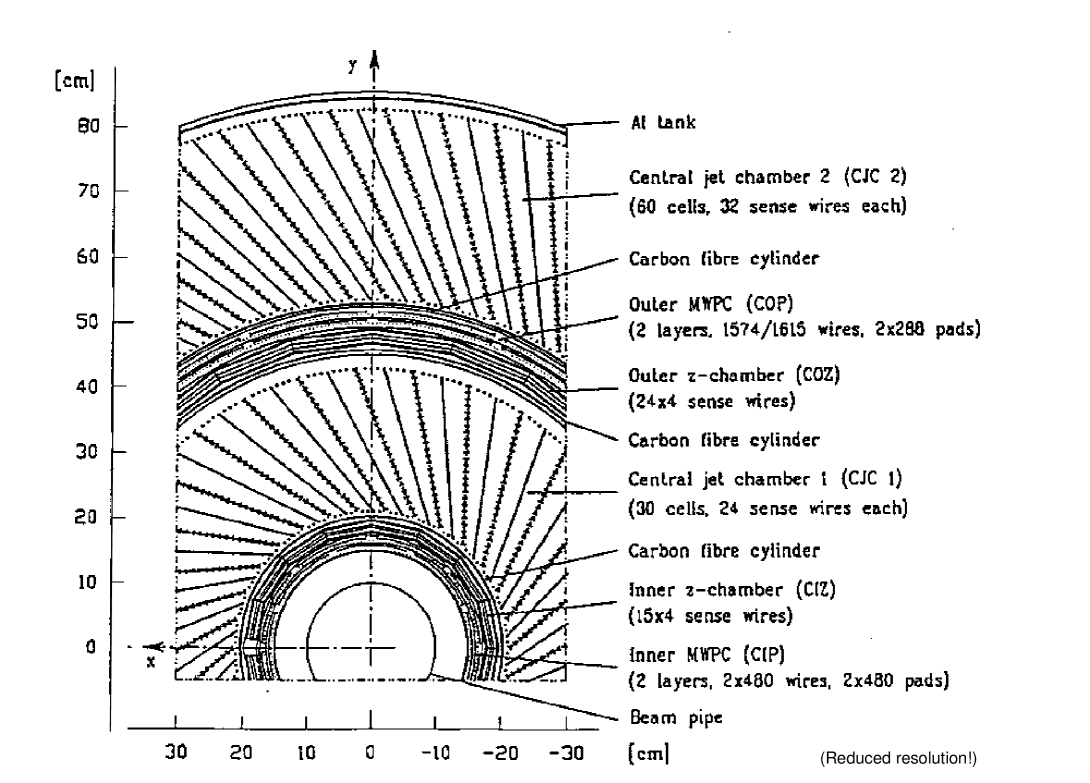
Abbildung 2.4: Central tracking system, section perpendicular to the beam [10].

Abbildung 2.5: Transverse view of the stack segmentation of the BEMC [10].

Abbildung 2.6: The orientation of the absorber plates (top) and the cell structure of the LAr in $(r,z)$-view (bottom).

Kapitel 3 Deep-Inelastic Scattering

3.1 The Kinematics

Due to the high beam energies of $E_{e}=27.5\,{\rm GeV}$ and $E_{p}=820\,{\rm GeV}$ available at HERA, the masses of the electron and proton can safely be neglected for most purposes. This will be done throughout this study. Their four-momenta, indicated in fig. 3.1, can therefore be written as $k=(E_{e},0,0,p_{z_{e}})=(27.5,0,0,-27.5)\,{\rm GeV}$ and $P=(E_{p},0,0,p_{z_{p}})=(820,0,0,820)\,{\rm GeV}$ with $k^{2}=P^{2}=0$. Thus, the center of mass energy $\sqrt{s}$ follows from

$$s:=(k+P)^{2}=2k\cdot P=4E_{e}E_{p}=90200\,{\rm GeV}^{2}$$ (3.1)

to be $300.33\,{\rm GeV}$.

\psfrag{s}{$\hat{\sigma}$}\psfrag{S}{$\hat{\rm s}$}\psfrag{|}{$\left.\mbox{\rule{0.0pt}{48.0pt}}\right\}$}\includegraphics{epDIS}

Abbildung 3.1: Diagram of the basic $ep$ DIS process via neutral currents. The letters in parentheses label the corresponding four-momenta.

The Neutral Current (NC) interaction displayed in fig. 3.1 is mediated via the exchange of a virtual $\gamma$ or $Z^{0}$ boson with four-momentum $q=k-k^{\prime}$ and mass $q^{2}<0$ where $k^{\prime}$, the four-momentum of the outgoing electron, may be chosen to be $k^{\prime}=(E_{e^{\prime}},E_{e^{\prime}}\sin\theta_{e^{\prime}},0,E_{e^{\prime}}\cos\theta_{e^{\prime}})$, i.e. $\phi_{e^{\prime}}:=0$. Charged Current (CC) reactions involving $W^{\pm}$ bosons would yield an outgoing neutrino $\nu_{e}$ and will not be considered here. In the case of elastic scattering $ep\rightarrow ep$, the Lorentz invariant momentum transfer squared

$$Q^{2}:=-q^{2}=-(k-k^{\prime})^{2}=2k\cdot k^{\prime}=2E_{e}E_{e^{\prime}}(1+\cos{\theta_{e^{\prime}}})$$ (3.2)

would suffice to characterize the process. Protons, however, are not point-like particles, but have a complex internal structure revealing itself at distances of ${\scriptstyle\lesssim}\,1\,{\rm fm}$, equivalent to $Q^{2}\,{\scriptstyle\gtrsim}\,0.04\,{\rm GeV}^{2}$. As consequences the proton, represented by the lower blob in fig. 3.1, on the one hand has to be described in terms of structure functions, and on the other hand it usually breaks up since elastic reactions are strongly suppressed compared to inelastic ones with increasing $Q^{2}$ [1]. This inevitably leads to the need of another quantity to define the global outcome of an event, i.e. without differentiating the hadronic final state. Looking at the photon-proton ($\gamma^{*}p$) interaction by itself, we have only one additional invariant at our disposal:

$$W^{2}:=(q+P)^{2}=2P\cdot q-Q^{2},$$ (3.3)

which is limited by $0\leq W^{2}\leq s$.

Other popular choices are the two dimensionless variables

$$x := \frac{Q^{2}}{2P\cdot q}\,,$$ (3.4)

$$y := \frac{P\cdot q}{P\cdot k}$$ (3.5)

with the neat property that $0\leq(x,y)\leq 1$. In the context of the infinite momentum frame, where the proton is conceived of as a collinear stream of fast moving partons and masses are negligible, $x$ can be interpreted as the fraction of the total momentum carried by the struck constituent as seen from the virtual boson. This reference frame has implicitly been adopted in fig. 3.1 as the hard scattering with a parton, labelled $\hat{\sigma}$ with mass $\sqrt{\hat{s}}$, is assumed to be incoherent and well separated from ensuing soft processes. In the simplest situation of a boson-parton collision where

$$\hat{s}:=(q+\xi P)^{2}=2\xi q\cdot P-Q^{2}=\left(\frac{\xi}{x}-1\right)Q^{2}$$ (3.6)

vanishes, $x$ is identical to $\xi$ of fig. 3.1 according to

$$\xi=\left(1+\frac{\hat{s}}{Q^{2}}\right)x\,.$$ (3.7)

Under more complex circumstances with $\hat{s}>0$, it can only be concluded that $x\leq\xi\leq 1$.

In fixed-target experiments, $y$ is easily interpreted as relative energy loss of the scattered lepton because in the rest frame of the target denoted by ^∙’s:

$$y=\frac{m_{p}(E^{\bullet}_{e}-E^{\bullet}_{e^{\prime}})}{m_{p}E^{\bullet}_{e}}=\frac{E^{\bullet}_{e}-E^{\bullet}_{e^{\prime}}}{E^{\bullet}_{e}}\,.$$ (3.8)

Of course, only two of the four introduced kinematic quantities are independent of each other. The conversion formulae for the pairs $(Q^{2},W^{2})\leftrightarrow(x,y)$ are:

$$x=\frac{Q^{2}}{Q^{2}+W^{2}}\,, \quad y=\frac{Q^{2}+W^{2}}{s}\,,$$

$$Q^{2}=sxy\,,\qquad\;\> W^{2}=s\,(1-x)\,y\,.$$

3.2 Reconstruction of the Kinematical Quantities

When confronted with real data, one has to reconstruct the kinematical quantities of an event from the measured energy depositions. Basically, we have four measurements at our disposal for the determination of two unknowns: the energies and polar angles of the scattered electron and the current jet, i.e. a collimated shower of hadrons produced by the struck parton: $E_{e^{\prime}}$, $\theta_{e^{\prime}}$, $E_{j}$, $\theta_{j}$. Depending on the choice of input variables, several reconstruction methods exist, each with specific advantages and drawbacks.

Abbildung 3.2: The two plots show the lines of constant energy (full lines) and polar angle (dashed) for the scattered electron (top) and the current jet (bottom) in an $(x,Q^{2})$-plane. Lines of constant $y$ (dotted except for $y=1$) are drawn for $y=1,10^{-1},10^{-2}$ and $10^{-3}$.

Fig. 3.2 presents the lines of constant energy and polar angle for the scattered electron and the current jet in the $(x,Q^{2})$-plane. Lines of constant $y=Q^{2}/(sx)$ are displayed for $y=1,10^{-1},10^{-2}$ and $10^{-3}$. For reconstruction purposes it is best if the isolines of a quantity are closely staggered and intersect the isolines of the corresponding second variable predominantly under large angles. Henceforth, the electron data alone are sufficient for a good determination of $Q^{2}$ in the complete range shown. The large gaps, however, between energies $E_{e^{\prime}}=25\,{\rm GeV}$ and $E_{e^{\prime}}=40\,{\rm GeV}$ and angles $\theta_{e^{\prime}}$ larger than $90{{}^{\circ}}$ demonstrate that the electron method is not very reliable for large $x$ or low $y$ respectively. Despite the fact that hadronic energies and angles have much larger uncertainties than electromagnetic ones, the current jet data can provide better estimates for $x$ or $y$ in that region.

Yet, because we are interested in the shape of the hadronic final state, we have to restrict ourselves mainly to the electron quantities in order not to bias our results. The application of a jet algorithm like the ones described in section 4.2.3 to obtain $E_{j}$ and $\theta_{j}$ is not advisable. Fortunately, there is also an inclusive method to derive the kinematics from hadronic measurements first proposed by Jacquet and Blondel [14]. Alternatively, one could rely on the angular measurements of the electron and the hadronic system alone [15]. These three methods will be presented in the next sections. For a comparison ref. [16] may be consulted.

3.2.1 The Electron Method

The electron method is the simplest possibility to extract $y$ and $Q^{2}$ and employs the scattered electron only. $x$ and $W^{2}$ can then be calculated according to eqs. (LABEL:eqn:conversion). Using the definitions (3.2) and (3.5), it follows directly:

$$y_{e}=1-\frac{P\cdot k^{\prime}}{P\cdot k}=1-\frac{E_{e^{\prime}}}{E_{e}}\frac{1-\cos\theta_{e^{\prime}}}{2}=1-\frac{E_{e^{\prime}}-p_{z_{e^{\prime}}}}{2E_{e}}\,,$$ (3.10)

$$Q^{2}_{e}=2k\cdot k^{\prime}=2E_{e}E_{e^{\prime}}(1+\cos{\theta_{e^{\prime}}})=2E_{e}(E_{e^{\prime}}+p_{z_{e^{\prime}}})=\frac{p_{t_{e^{\prime}}}^{2}}{1-y_{e}}\,.$$ (3.11)

3.2.2 The Jacquet-Blondel Method

With $h$ representing the four-momentum of the complete hadronic final state, it is clear from fig. 3.1 that $q=k-k^{\prime}=h-P$. Furthermore, $p_{t}$-balance enforces $p_{t_{h}}=p_{t_{e}}$ so that

$$y_{h}=\frac{P\cdot(h-P)}{P\cdot k}=\frac{\sum\limits_{i}\left(E_{i}-p_{z_{i}}\right)}{2E_{e}}\,,$$ (3.12)

$$Q^{2}_{h}=\frac{p^{2}_{t_{h}}}{1-y_{h}}=\frac{\left(\sum\limits_{i}p_{x_{i}}\right)^{2}+\left(\sum\limits_{i}p_{y_{i}}\right)^{2}}{1-y_{h}}$$ (3.13)

where $i$ loops over all hadronic objects.

3.2.3 The Double Angle Method

Requiring $y_{h}=y_{e}$ and $p_{t_{h}}=p_{t_{e^{\prime}}}$, the dependence on $E_{e^{\prime}}$ and $\sum_{i}E_{i}$ for all hadrons $i$ can be eliminated such that:

$$y_{da}=\frac{\sin\theta_{e^{\prime}}(1-\cos\theta_{h})}{\sin\theta_{e^{\prime}}(1-\cos\theta_{h})+\sin\theta_{h}(1-\cos\theta_{e^{\prime}})}\,,$$ (3.14)

$$Q^{2}_{da}=4E_{e}^{2}\frac{\sin\theta_{h}(1+\cos\theta_{e^{\prime}})}{\sin\theta_{e^{\prime}}(1-\cos\theta_{h})+\sin\theta_{h}(1-\cos\theta_{e^{\prime}})}\,.$$ (3.15)

3.3 The Born Cross Section

To derive a cross section formula for deep-inelastic $ep\rightarrow eX$ scattering, it will be required that the total process can be separated into a two step procedure. In the first part, involving very small space-time scales of ${\cal O}(1/Q)$ where the strong interaction is weak, the basic kinematic outcome of a reaction is fixed by the incoherent elastic scattering of the boson probe and a proton constituent. The ensuing soft hadronization of the struck parton and the proton remnant takes place at a time scale typically of the order of inverse hadron masses $1/M$ with $M\approx 200\,{\rm MeV}\ll Q$ instead and merely affects the detailed structure of the hadronic final state.

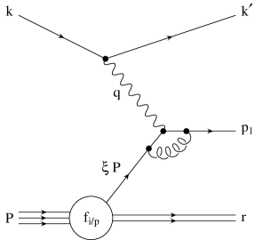
Abbildung 3.3: Quark-Parton-Model Feynman graph (left) and an example of a virtual correction to it (right).

Without resolving such details, it is therefore possible to calculate a cross section by applying perturbation theory in lowest or Leading Order (LO, here: ${\cal O}(\alpha^{2}\alpha_{s}^{0})$) to the hard subprocess $\hat{\sigma}$ of fig. 3.1. The blob is then replaced by a single boson-parton vertex as shown in the Quark-Parton-Model (QPM) Feynman diagram of fig. 3.3. If the proton itself is left out, essentially an elastic two-body scattering reaction remains for which the cross sections have been calculated, s. e.g. [1]. One possibility to derive a general cross section formula is to assume partons with spin $1/2$ and $0$ [1]. Depending on the spin, one takes over the result from $e\mu$ respectively $e\pi$ scattering:

$$\frac{d\sigma^{e\mu}}{dQ^{2}} = \frac{2\pi\alpha^{2}}{Q^{4}}(1+(1-y)^{2})\,,$$ (3.16)

$$\frac{d\sigma^{e\pi}}{dQ^{2}} = \frac{4\pi\alpha^{2}}{Q^{4}}(1-y)\,.$$ (3.17)

Here, $\alpha$ denotes the electromagnetic coupling strength and NC contributions from $Z^{0}$ exchange, which are suppressed at least $\propto Q^{2}/(Q^{2}+M_{Z}^{2})$, are neglected.

At this stage, we must again consider the internal arrangement of partons in the proton that can be parameterized in the form of parton density functions (pdfs) $f_{i/p}(x)$ which represent the probability to find a constituent $i$ with a momentum fraction in the interval $[x,x+dx]$. Denoting the spin-$1/2$ pdfs with $f_{i/p}(x)$ and the spin-$0$ ones with $f_{j/p}(x)$, the differential cross section can be written as

$$\frac{d\sigma^{ep}}{dQ^{2}}=\frac{4\pi\alpha^{2}}{Q^{4}}\left(\frac{1+(1-y)^{2}}{2}\sum\limits_{i}q_{i}^{2}f_{i/p}(x)dx+(1-y)\sum\limits_{j}q_{j}^{2}f_{j/p}(x)dx\right)\,,$$ (3.18)

where $q_{i}$ and $q_{j}$ are the corresponding electromagnetic charges of the constituent flavours $i$ and $j$ in units of the positron charge. Historically, the derivation of the cross section implied the evaluation of a leptonic tensor $L^{\mu\nu}$ prescribed by QED and its contraction with the most general form of a hadronic tensor $W_{\mu\nu}$ describing the hadronic vertex. This approach, employed e.g. in [2, 4], led to the definition of structure functions $F_{1}(x)$ and $F_{2}(x)$ which here translate to

$$F_{1}(x) = \sum\limits_{i}\frac{1}{2}q_{i}^{2}f_{i/p}(x)\,,$$ (3.19)

$$F_{2}(x) = \sum\limits_{i}q_{i}^{2}xf_{i/p}(x)+\sum\limits_{j}q_{j}^{2}xf_{j/p}(x)\,.$$ (3.20)

The double differential cross section (3.18) now reads

$$\frac{d^{2}\sigma^{ep}}{dQ^{2}dx}=\frac{4\pi\alpha^{2}}{xQ^{4}}\left((1-y)F_{2}(x)+xy^{2}F_{1}(x)\right)\,.$$ (3.21)

So far the partons served as a term for point-like constituents within the proton that lead to the experimentally observed $1/Q^{4}$-dependence of the inelastic cross section in contrast to the dramatic $1/Q^{12}$-decrease for elastic reactions. Combining this with the quark model by identifying partons and spin-$1/2$ quarks, one immediately concludes that $f_{j/p}(x)\equiv 0\,\forall j$ and henceforth

$$F_{2}(x)=2xF_{1}(x)\,.$$ (3.22)

This is the experimentally well established Callan-Gross relation which demonstrates the fermionic nature of the charged proton constituents. In addition, one can conclude from eq. (3.21) that the cross section normalized to the corresponding one for point-like particles depends on the scaling variable $x$ only. The observation of deviations can be attributed to the neglect of masses, intrinsic transverse momenta and — most importantly — the strong interaction.

3.4 The NLO Cross Section

Up to now, the proton was treated like a stream of collinear non-interacting quarks. However, in Next-to-Leading Order (NLO), i.e. ${\cal O}(\alpha^{2}\alpha_{s}^{1})$, quarks can emit and absorb gluons which again may split up into two gluons or $q\bar{q}$ pairs and so forth. The rather simple picture involving structure functions $F_{1}(x)$, $F_{2}(x)$ to describe the composition of the proton in terms of quark densities alone has to be modified accordingly to include a gluon density. Two of the most important consequences are scaling violations, i.e. a dependence of $F_{1}(x),F_{2}(x)$ on $Q^{2}$, and non-vanishing contributions to the longitudinal structure function

$$F_{L}:=F_{2}-2xF_{1}\,.$$ (3.23)

For low $x$, i.e. $x\,\lesssim\,10^{-3}$, approximations reveal the effects to be proportional to $\alpha_{s}(Q^{2})$ times the gluon density $g(x,Q^{2})$:

$$\frac{dF(x,Q^{2})}{d\log Q^{2}}\propto\alpha_{s}(Q^{2})\cdot g(x,Q^{2})\,,$$ (3.24)

$$F_{L}(x,Q^{2})\propto\alpha_{s}(Q^{2})\cdot g(x,Q^{2})\,.$$ (3.25)

Both are intensively studied in DIS experiments and can be exploited in inclusive measurements to gain information on the strong coupling constant as well as the gluon density. For H1 publications on this topic consult refs. [17, 18].

In this analysis all hadronic final states are considered but will be differentiated with respect to suitably chosen characteristic variables (s. section 4.2), i.e. the measurement is semi-inclusive.

To ${\cal O}(\alpha_{s}^{1})$ there are two kinds of processes resulting in two instead of one final state parton, where “parton” from now on is used synonymously for quarks, anti-quarks and gluons. Since they may lead to “real” effects like an additional jet they are called real corrections. In the first case of the QCD-Compton graphs (QCDC), an additional gluon is emitted by the struck quark. The two possible Feynman diagrams are presented in fig. 3.4.

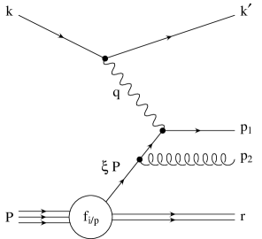
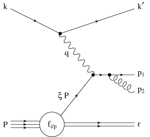
Abbildung 3.4: QCD-Compton Feynman graphs.

The second kind with diagrams shown in fig. 3.5 involves the production of a $q\bar{q}$ pair from a reaction between the boson and a gluon emitted from the proton. They are expressively labelled Boson-Gluon-Fusion graphs (BGF).

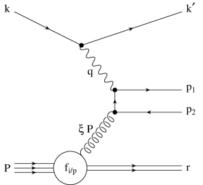
Abbildung 3.5: Boson-Gluon-Fusion Feynman graphs.

To complete the set of contributions to $ep$ DIS to ${\cal O}(\alpha_{s}^{1})$, one also has to consider loop diagrams. One example is given on the right-hand side of fig. 3.3. The diagram itself results in an ${\cal O}(\alpha_{s}^{2})$ add-on to the matrix element squared. However, since the final states of both graphs in fig. 3.3 are indistinguishable, an interference term of ${\cal O}(\alpha_{s}^{1})$ has to be taken into account. For the purpose of differentiating the hadronic final state, this virtual correction is, of course, irrelevant and merely changes the total cross section.

Focusing on the two-parton QCDC and BGF processes, three new degrees of freedom arise in the matrix elements corresponding to energy, azimuthal and polar angle of one parton. The other parton is then determined by energy-momentum conservation. Usually, the now five-fold differential cross section is written employing the variables

$$x_{p} := \frac{Q^{2}}{2\,(\xi P)\cdot q}=\frac{x}{\xi}\,,$$ (3.26)

$$z_{p} := \frac{P\cdot p_{1}}{P\cdot q}=1-\frac{P\cdot p_{2}}{P\cdot q}\,,$$ (3.27)

and $\phi$, where $\phi$ denotes the angle between the planes fixed by the two outgoing partons on the one hand, and the scattered electron on the other hand in a suitable reference frame. This may be e.g. the Breit frame defined in the next chapter or any other reference system connected to it by a Lorentz boost along its $z$-direction. Concerning the characterization of the hadronic final state, no reference will be made to the electron. Therefore, the integration over $\phi$ can be performed beforehand such that for our purposes the NLO cross section may be labelled as

$$\frac{d^{4}\sigma^{ep}}{dQ^{2}dxdx_{p}dz_{p}}\,.$$ (3.28)

The allowed ranges for $x_{p}$ and $z_{p}$ are $x\leq x_{p}\leq 1$ and $0\leq z_{p}\leq 1$.

Yet, it does contain singularities! For the QCDC and BGF processes they can be extracted from ref. [19], which presents the complete ${\cal O}(\alpha_{s}^{1})$ corrections to electroweak NC and CC $ep$ DIS cross sections, to be:

$$d\sigma^{\rm QCDC} \propto \frac{1+x_{p}^{2}z_{p}^{2}}{(1-x_{p})(1-z_{p})}\,,$$ (3.29)

$$d\sigma^{\rm BGF} \propto \frac{[x_{p}^{2}+(1-x_{p})^{2}][z_{p}^{2}+(1-z_{p})^{2}]}{z_{p}(1-z_{p})}\,.$$ (3.30)

Partially, they cancel against corresponding divergent terms of the virtual corrections. The remaining initial state mass singularities can be absorbed in a proper redefinition of the parton densities. Nevertheless, one has to be careful about the precise definition of quantities that shall be calculated by pQCD. In order to allow the divergences to compensate each other, the investigated variables must agree in the limits where the real and virtual corrections go to infinity. The number of final state particles for example would always be two in the first case and one in the latter.

To be more definite, we make use of eqs. (4.30)–(4.34) and can refer the limits $x_{p}\rightarrow 1$ and $z_{p}\rightarrow 0,1$ to configurations where either $p_{1}$ or $p_{2}$ are soft (infrared divergence) or any pair of $\{p_{1},p_{2},r\}$ is collinear (collinear divergence). Hence, any quantity $F_{n}({\rm\vec{p}}_{1},\ldots,{\rm\vec{p}}_{n})$ to be meaningful in pQCD has to fulfil the conditions

$$F_{n}({\rm\vec{p}}_{1},\ldots,\lambda{\rm\vec{p}}_{i},\ldots,{\rm\vec{p}}_{j}=(1-\lambda){\rm\vec{p}}_{i},\ldots,{\rm\vec{p}}_{n}) = F_{n-1}({\rm\vec{p}}_{1},\ldots,{\rm\vec{p}}_{i},\ldots,{\rm\vec{p}}_{j-1},{\rm\vec{p}}_{j+1},\ldots,{\rm\vec{p}}_{n})$$ (3.31)

$${\rm and}$$

$$\lim_{\lambda\rightarrow 0}F_{n}({\rm\vec{p}}_{1},\ldots,\lambda{\rm\vec{p}}_{i},\ldots,{\rm\vec{p}}_{n}) = F_{n-1}({\rm\vec{p}}_{1},\ldots,{\rm\vec{p}}_{i-1},{\rm\vec{p}}_{i+1},\ldots,{\rm\vec{p}}_{n})$$

for $0<\lambda<1$. That is, collinear splittings and soft particles do not affect $F$; it is collinear and infrared safe. One example for such a variable is thrust, or rather $1-$thrust, defined by eq. (4.9). It is invariant with respect to collinear splittings and varies smoothly for one momentum approaching zero.

Kapitel 4 Event Shapes

4.1 The Breit Frame

4.1.1 Introduction

Initially, all energy deposits measured with the H1 detector are given in the laboratory system. Since we are, however, merely interested in specific properties of the hadronic final state caused by the hard interaction, two problems arise:

1. The transverse momentum of the scattered electron is balanced by the hadronic system. Hence, from longitudinal and transverse momenta of the hadrons one can reconstruct the global event kinematics, but they are not characteristic of the underlying hadronic process.

2. Somehow we have to differentiate between the products of the hard reaction and the proton remnant. A maximal separation, which is not given in the laboratory system, is desirable.

For illustration fig. 4.1 shows a comparatively simple NC event with a clearly identifiable electron and a lot of hadronic activity on the opposite side with respect to $\phi$. In addition, the proton rest manifests itself in the form of some clusters in the forward direction.

\psfrag{+zb}{$+z^{\star}$}\psfrag{-zb}{$-z^{\star}$}\psfrag{thetaq}{$\theta_{q}$}\psfrag{q2=3934}{$Q^{2}=3934\,{\rm GeV}^{2}$}\psfrag{y=0.318}{$y=0.318$}\psfrag{thetaq=37.3}{$\theta_{q}=37.3{{}^{\circ}}$}\psfrag{Ee=54.5}{$E_{e^{\prime}}=54.5\,{\rm GeV}$}\psfrag{phie=291.3}{$\phi_{e^{\prime}}=291.3{{}^{\circ}}$}\psfrag{thetae=71.9}{$\theta_{e^{\prime}}=71.9{{}^{\circ}}$}\includegraphics[width=455.24408pt]{NC1}

Abbildung 4.1: Example of an $ep$ collision measured with the H1 detector which resembles a QPM-like configuration. The isolated electromagnetic cluster in the LAr with one track linked to it represents the scattered electron, whereas the broader energy deposits in the upper half of the LAr balance the electron $p_{t}$ and correspond to a jet of hadrons produced by the struck quark. Some energy measured in the very forward direction indicates the proton remnant. The basic kinematic quantities deduced from the electron are given.

Here already, it is not too obvious how to define characteristic properties of the hadronic energy deposits. In the case of much more complicated average events, it becomes forbidding. The solution to the two problems is to apply a Lorentz transformation into the Breit frame of reference [20]. For an event of QPM type as shown in fig. 4.2, it is defined as the reference system where the incoming parton with momentum $xP^{\star}$ in $+z^{\star}$-direction is back-scattered by a purely space-like boson of momentum $q^{\star}$.

From $q{{}^{\star}}^{2}=q^{2}=-Q^{2}$ and $xP^{\star}+q^{\star}=-xP^{\star}$, it follows that

$$q^{\star}=(0,0,0,-Q)$$ (4.1)

and

$$P^{\star}=\left(\frac{Q}{2x},0,0,\frac{Q}{2x}\right)$$ (4.2)

where $Q$ is defined to be

$$Q:=\sqrt{-q^{2}}=\sqrt{Q^{2}}\,.$$ (4.3)

Abbildung 4.2: Diagram of a QPM-type $ep$ collision as seen in the Breit frame.

Thereby, the event and also the “soft” and “hard” physics is separated by the $(x^{\star},y^{\star})$-plane into a $+z^{\star}$ Remnant Hemisphere (RH) and a $-z^{\star}$ Current Hemisphere (CH). Simultaneously, the transverse momentum of the scattered quark has been eliminated such that the CH with its available energy of $Q/2$ is very similar to one half of an $e^{+}e^{-}\rightarrow q\bar{q}$ event with purely “time-like” energy $\sqrt{s}/2$, relating the “relevant energies” $Q$ and $\sqrt{s}$.

Technically, the necessary Lorentz transformation is decomposed into a pure boost demanding that

$$2xP^{\star}+q^{\star}=\left(\begin{array}[]{c}Q\\ {\rm\vec{0}}\end{array}\right)$$ (4.4)

and a rotation afterwards to readjust $P^{\star}$ into the $+z^{\star}$-direction. In addition, the incoming and outgoing electron is usually required to lie in the $(x^{\star},z^{\star})$-plane. Their boosted and rotated four-momenta read

$$k^{\star}=\left(\frac{Q}{2y}(2-y),\frac{Q}{y}\sqrt{1-y},0,-\frac{Q}{2}\right)$$ (4.5)

and

$$k{{}^{\star}}^{\prime}=\left(\frac{Q}{2y}(2-y),\frac{Q}{y}\sqrt{1-y},0,\frac{Q}{2}\right)\,.$$ (4.6)

Thus, another feature of the Breit frame is that the energy loss of the lepton, $E_{e}^{\star}-E_{e}{{}^{\star}}^{\prime}$, vanishes.

4.1.2 Properties

For a better clarification of what happens to the clusters in fig. 4.1, we introduce another variable $\theta_{q}$ which corresponds to the polar angle of the scattered quark as seen by the electron:

$$\cos\theta_{q}=\frac{Q_{e}^{2}\,(1-y_{e})-4y_{e}^{2}E_{e}^{2}}{Q_{e}^{2}\,(1-y_{e})+4y_{e}^{2}E_{e}^{2}}\,.$$ (4.7)

A comparison of $\theta_{q}$, drawn also in fig. 4.1, with the polar angle of the most energetic hadronic energy deposition in the LAr obviously demonstrates that they are approximately equal. When looked at it from the Breit frame, the $+z$-axis remains at its position, but the new $-z^{\star}$-direction is given by $\theta_{q}$! As a result, the angular region of $0{{}^{\circ}}\leq\theta\leq\theta_{q}$ is stretched until $0{{}^{\circ}}\leq\theta^{\star}\leq 180{{}^{\circ}}$ and, together with the remaining $180{{}^{\circ}}-\theta_{q}$, the complete polar angular range for opposite $\phi$, including the electron and most of the proton remnant, is squeezed. Intermediate $\phi$ angles other from $\phi_{q}$ and $\phi_{e}$ with $\phi_{q}-\phi_{e}=180{{}^{\circ}}$ constitute the transitional domain between the two cases.

For all variables defined in the next section, the energies and polar angles of the transformed four-vectors are the important input quantities. Azimuthal angles with respect to that of the scattered electron, i.e. $\phi^{\star}_{e}=0{{}^{\circ}}$, are rather insignificant. In fig. 4.3 we therefore restrict ourselves to four plots showing the $\theta^{\star}(\theta,\phi)$-, $\theta^{\star}(\theta,E)$-, $E^{\star}(E,\phi)$- and $E^{\star}(E,\theta)$-functions for the sample boost of fig. 4.1. For simplicity, an exact balance in $p_{t}$ of the electron and the hadronic final state is assumed so that $E=85.5\,{\rm GeV}$ is taken as default.

Abbildung 4.3: The $\theta^{\star}(\theta,\phi)$- (top left), $\theta^{\star}(\theta,E)$- (top right), $E^{\star}(E,\phi)$- (bottom left) and $E^{\star}(E,\theta)$-functions (bottom right) for the sample boost of fig. 4.1. The third input variable is set to $E=85.5\,{\rm GeV}$, $\phi=\phi_{q}=111.3{{}^{\circ}}$, $\theta=\theta_{q}=37.3{{}^{\circ}}$ and again $\phi=\phi_{q}$ respectively.

From these plots it can be concluded that:

1. $\theta^{\star}(\theta,\phi)$ peaks sharply at $(\theta_{q},\phi_{q})$.

2. Only clusters opposite of the electron hemisphere in the laboratory system appear in the CH, i.e. $\theta^{\star}>90{{}^{\circ}}$.

3. $\theta^{\star}$ is independent of the energy of the boosted vector.

4. $E^{\star}\propto E$ with the slope strongest at $\phi_{e}$ and $\theta=180{{}^{\circ}}$.

The first property may lead to a serious deterioration of the resolution in polar angle in the Breit frame and is the motivation for the cut-off no. • ‣ 5.5 introduced in section 5.5.

4.2 Definition of the Event Shapes

According to fig. 4.2, the hadronic final state in the simplest case consists of merely one parton with longitudinal momentum only and no mass. The hard interaction is of a purely electromagnetic nature. QCD induces deviations from this constellation. By investigating variables that are sensitive to these deviations, it is possible to learn more about perturbative and non-perturbative aspects of QCD.

All quantities, introduced in the next sections and generically labelled as $F$, are event shapes and have the following properties in common:

1. They are dimensionless.

2. For $ep$ DIS they are defined in the Breit frame of reference.

3. In the limit of a QPM-like event $F=0$, otherwise $F\geq 0$.

4. They are infrared and collinear safe, which is most important for a valid comparison with pQCD.

5. Soft fragmentation and hadronization processes cause discrepancies between fixed-order pQCD calculations and measured data that generally can be parameterized to be $\propto 1/Q^{p}$ with $Q$ being the relevant energy scale and $p=1$ or $p=2$ in our circumstances.

The event shapes discussed in the next two subsections assume that the hard subprocess takes place in the CH alone. However, for $\xi>2x$ it is possible for the CH to be completely empty, although experimentally this is improbable due to hadronization, backscattering, noise, etc. In order to be insensitive to such effects and to remain infrared safe [22], one has to specify what is meant by an “empty” or, vice versa, a “full” CH. We adopt the prescription that the total energy available in the CH $E^{\star}:=\sum_{\scriptscriptstyle i\in{\rm CH}}E_{i}^{\star}$ has to exceed $20\%$ of the value it should have according to QPM:

$$E^{\star}>0.2\cdot Q/2=Q/10\,.$$ (4.8)

Otherwise the event is ignored. The precise value of the cut-off is motivated by a study of the measured energy flow in both hemispheres performed for ref. [23].

To keep event shapes dimensionless, it was originally suggested in [24] to normalize energies, momenta and masses to $Q/2$. “Empty” events would then lead to $F=0$. Following the proposal in [25] to use for experimental reasons the actually present total energy $E^{\star}$ or momentum $P^{\star}:=\sum_{\scriptscriptstyle i\in{\rm CH}}|{\rm\vec{p}}_{i}{{}^{\star}}|$ instead, one would get ill-defined expressions. Therefore, $F$ is set to zero in [21] analogously for this normalization in contrast to our definition, thereby affecting the total cross section $\sigma$ and the left-most bin of the differential cross section $d\sigma/dF$. Except for the difference in $\sigma$, mean values $\left<F\right>$, however, are not altered. In this work, we will mainly restrict ourselves to the study of the event shapes normalized to $E^{\star}$ or $P^{\star}$.

Note that in contrast to the first published experimental results on event shapes in $ep$ DIS [25, 23] we adopt the modified naming scheme from ref. [21]. Except for $\tau_{C}$ defined below, the subscript indicates the quantity ($E$, $P$ or $Q$) used for the normalization. The event shapes $1-T_{C}$, $1-T_{Z}$, $B_{C}$ and $\rho_{C}$ investigated in the above-mentioned publications will be labelled $\tau_{C}$, $\tau_{P}$, $B_{P}$ and $\rho_{Q}$.

4.2.1 Event Shapes employing $z^{\star}$ as Event Axis

Choosing the direction of the exchanged boson ${\rm\vec{q}}_{\leavevmode\nobreak\ }{{}^{\star}}=(0,0,-Q)$ as event axis ${\rm\vec{n}}$, one can, with fig. 4.2 in mind, easily deduce quantities $F$ being zero for QPM-like configurations and $F>0$ otherwise. The simplest event shapes thrust (or rather $1-$thrust $\tau:=1-T$) and jet broadening $B$ can be written as [26, 24, 25]

$$\tau_{P}:=1-\frac{\sum\limits_{\scriptscriptstyle i\in{\rm CH}}\left|{\rm\vec{p}}_{i}{{}^{\star}}\cdot{\rm\vec{n}}\right|}{\sum\limits_{\scriptscriptstyle i\in{\rm CH}}\left|{\rm\vec{p}}_{i}{{}^{\star}}\right|}=1-\frac{\sum\limits_{\scriptscriptstyle i\in{\rm CH}}\left|p_{li}^{\star}\right|}{P^{\star}}\,, \tau_{Q}:=1-\frac{\sum\limits_{\scriptscriptstyle i\in{\rm CH}}\left|p_{li}^{\star}\right|}{Q/2}\,,$$ (4.9)

$$B_{P}:=\frac{\sum\limits_{\scriptscriptstyle i\in{\rm CH}}\left|{\rm\vec{p}}_{i}{{}^{\star}}\times{\rm\vec{n}}\right|}{2\sum\limits_{\scriptscriptstyle i\in{\rm CH}}\left|{\rm\vec{p}}_{i}{{}^{\star}}\right|}=\frac{\sum\limits_{\scriptscriptstyle i\in{\rm CH}}\left|p_{ti}^{\star}\right|}{2P^{\star}}\,,\qquad\quad B_{Q}:=\frac{\sum\limits_{\scriptscriptstyle i\in{\rm CH}}\left|p_{ti}^{\star}\right|}{Q}$$ (4.10)

where $p_{l}$ and $p_{t}$ denote the longitudinal respectively the transversal momentum components of ${\rm\vec{p}}$. The factor of $1/2$ for $B$ is conventional.

4.2.2 Event Shapes without Reference to $z^{\star}$ as Event Axis

A possibility for differentiation without reference to $z^{\star}$ as event axis is given by the jet mass $\rho$ [27]:

$$\rho_{E}:=\frac{\left(\sum\limits_{\scriptscriptstyle i\in{\rm CH}}p_{i}^{\star}\right)^{2}}{4\left(\sum\limits_{\scriptscriptstyle i\in{\rm CH}}E_{i}^{\star}\right)^{2}}=\frac{M^{2}}{4E{{}^{\star}}^{2}}\,,\qquad\qquad\, \rho_{Q}:=\frac{M^{2}}{Q^{2}}$$ (4.11)

with $M$ being the total mass in the CH.

Another way is the evaluation with respect to a new axis to be defined. Originally, event shapes were introduced in the context of $e^{+}e^{-}$  annihilations, where, in distinction to $ep$ DIS, a preferred direction like $z^{\star}$ is not given beforehand. The first definition deals with the thrust axis ${\rm\vec{n}}_{T}$ which is characterized as the normalized vector that maximizes the sum of all projections of momenta (absolute values) onto it. With regard to that, $\tau=1-$thrust can now be described as

$$\tau_{C}:=1-\max_{{\rm\vec{n}},{\rm\vec{n}}^{2}=1}\frac{\sum\limits_{\scriptscriptstyle i\in{\rm CH}}\left|{\rm\vec{p}}_{i}{{}^{\star}}\cdot{\rm\vec{n}}\right|}{\sum\limits_{\scriptscriptstyle i\in{\rm CH}}\left|{\rm\vec{p}}_{i}{{}^{\star}}\right|}=1-\frac{\sum\limits_{\scriptscriptstyle i\in{\rm CH}}\left|{\rm\vec{p}}_{i}{{}^{\star}}\cdot{\rm\vec{n}}_{T}\right|}{P^{\star}}\,.$$ (4.12)

In contrast to $e^{+}e^{-}$ physics, the maximizing procedure is applied in the CH alone. For merely one momentum vector, $\tau_{C}$ always equals zero.

A second kind of event axis brings the momentum tensor

$$\Theta_{jk}^{\star}:=\frac{\sum\limits_{\scriptscriptstyle i\in{\rm CH}}\frac{p_{j_{i}}^{\star}p_{k_{i}}^{\star}}{\left|{\rm\vec{p}}_{i}^{\star}\right|}}{\sum\limits_{\scriptscriptstyle i\in{\rm CH}}\left|{\rm\vec{p}}_{i}^{\star}\right|}$$ (4.13)

into play. This real symmetric matrix is positive semi-definite with trace $Tr(\Theta)=\lambda_{1}+\lambda_{2}+\lambda_{3}=1$. For $0<\lambda_{3}\leq\lambda_{2}\leq\lambda_{1}<1$ it describes an ellipsoïd with pairwise orthogonal axes named minor, semi-major and major with increasing eigenvalue. The major axis is similar but not identical to ${\rm\vec{n}}_{T}$. If $\lambda_{3}=0$, then the ellipsoïd degenerates into an elliptical cylinder with all momentum vectors in one plane. Is $\lambda_{2}=0$ as well, then all momenta are collinear and the corresponding normal area consists of one or two parallel planes. Utilizing the eigenvalues, we can define the $C$ parameter [28]:

$$C_{P}:=3(\lambda_{1}\lambda_{2}+\lambda_{2}\lambda_{3}+\lambda_{3}\lambda_{1})\,, C_{Q}:=\frac{4P{{}^{\star}}^{2}}{Q^{2}}C_{P}\,.$$ (4.14)

The conventional factor of three ensures a maximal value of one for $C_{P}$.

4.2.3 Event Shapes employing Jet Algorithms for the Separation of the Remnant

Another approach of characterizing an event with regard to deviations from the QPM type does not make use of the CH. As depicted in section 3.1, the elementary reaction yields one hard parton moving along the $-z^{\star}$-direction. The ensuing production of soft partons during fragmentation and the final hadronization distort this picture to a limited extent only since no large transverse momenta with respect to the original one are involved. Basically, the one parton gets transformed into a tight stream of hadrons, flying along the original direction, which one refers to as a jet.

The inclusion of more complex processes into the pQCD calculation facilitates the production of two or more hard partons (s. section 3.4), and henceforth the events can acquire more than one jet in addition to the remnant jet. QPM-like events may also be called to be of a $(1+1)$-jet type in contrast to $(n+1)$-jet events with $n\geq 2$. In order to decide to which category a given constellation belongs, precise instructions on how to combine jets from an assortment of four-momenta are needed. The most basic of these jet algorithms [29] makes use of angular cones around seeds given by the input four-vectors. The two schemes we employ are of another type called cluster algorithms. Both, the Durham- or $k_{t}$- [30, 31] and the JADE-algorithm [32, 33] are applied in a modified form adapted to $ep$ DIS in the Breit frame.

The central procedure is almost the same for both. Two distance measures are defined, one for distances between two four-vectors, $y_{ij}$, and another one for the separation of each from the remnant, $y_{ir}$. When all combinations are evaluated, the minimal value determines which are the closest two in $y$. If an $y_{ij}$ was smallest, then these two are recombined to one new four-vector. In case of $y_{ir}$ to be minimal, $i$ is ascribed to the remnant. The whole routine is repeated until either all $y$’s are larger than a lower bound $y_{\rm cut}$, or until a certain number of jets is reached. The first prescription is used to divide a sample of reactions into sets of $(1+1)$-, $(2+1)$- and so forth events. The second approach is taken to employ $y$ as an event shape variable. Here, $y_{k_{t}}$ and $y_{fJ}$ always denote the $y$-value where the transition $(2+1)\rightarrow(1+1)$ occurs. The respective distance measures are

$$y_{ij} := \frac{2E_{i}^{\star}E_{j}^{\star}(1-\cos\theta_{ij}^{\star})}{Q^{2}}\,,$$ (4.15)

$$y_{ir} := \frac{2E_{i}^{\star}xE_{p}^{\star}(1-\cos\theta_{i}^{\star})}{Q^{2}}$$ (4.16)

for the factorizable JADE-algorithm and

$$y_{ij} := \frac{2\min(E_{i}{{}^{\star}}^{2},E_{j}{{}^{\star}}^{2})(1-\cos\theta_{ij}^{\star})}{Q^{2}}\,,$$ (4.17)

$$y_{ir} := \frac{2E_{i}{{}^{\star}}^{2}(1-\cos\theta_{i}^{\star})}{Q^{2}}$$ (4.18)

for the Durham-algorithm.

4.3 Event Shapes to ${\cal O}(\alpha_{s})$

As explained above, the event shapes are designed to distinguish between a QPM-like topology of the hadronic final state with the relevant cross section given by eq. (3.21) and deviations from it that are described in lowest order pQCD by eq. (3.28). In the first case, $F$ always equals zero, whereas in the latter, $F$ depends on the two additional degrees of freedom $x_{p}$ and $z_{p}$.

To derive explicit formulae, we first determine $p^{\star}_{1}$ and $p^{\star}_{2}$ from

$$p^{\star}_{1}+p^{\star}_{2}=\xi P^{\star}+q{{}^{\star}}=\left(\begin{array}[]{c}\frac{Q}{2x_{p}}\\ 0\\ 0\\ \frac{Q}{2x_{p}}-Q\end{array}\right)$$ (4.19)

according to eqs. (4.1) and (4.2). Remembering that azimuthal angles are irrelevant, we define the $y$-components to be zero such that

$$p^{\star}_{1}:=\frac{Q}{2}\left(\begin{array}[]{c}z_{0}\\ z_{t}\\ 0\\ z_{3}\end{array}\right)\,, p^{\star}_{2}:=\frac{Q}{2}\left(\begin{array}[]{c}\bar{z}_{0}\\ -z_{t}\\ 0\\ \bar{z}_{3}\end{array}\right)\,.$$ (4.28)

Using $p^{\star 2}_{1}=p^{\star 2}_{2}=0$ and

$$z_{p}=\frac{p^{\star}_{1_{0}}-p^{\star}_{1_{3}}}{Q}=\frac{z_{0}-z_{3}}{2}=1-\frac{\bar{z}_{0}-\bar{z}_{3}}{2}\,,$$ (4.29)

one can calculate $z_{0}$, $\bar{z}_{0}$, $z_{t}$, $z_{3}$ and $\bar{z}_{3}$ to be

$$z_{0} = \frac{2x_{p}z_{p}-x_{p}-z_{p}+1}{x_{p}}\,,$$ (4.30)

$$\bar{z}_{0} = \frac{-2x_{p}z_{p}+x_{p}+z_{p}}{x_{p}}\,,$$ (4.31)

$$z_{t} = 2\sqrt{\frac{z_{p}}{x_{p}}(1-x_{p})(1-z_{p})}\,,$$ (4.32)

$$z_{3} = \frac{1-x_{p}-z_{p}}{x_{p}}\,,$$ (4.33)

$$\bar{z}_{3} = \frac{z_{p}-x_{p}}{x_{p}}\,.$$ (4.34)

In the limit of $x_{p}\rightarrow 1$ and $z_{p}\rightarrow 1$ they evaluate to $z_{0}=1$, $z_{3}=-1$ and $\bar{z}_{0}=\bar{z}_{3}=z_{t}=0$ corresponding to a QPM-like event with only one final parton. Taking into account the mismatch in the sign of the $z^{\star}$-direction and noting that $x_{p}$ is named $\xi$ in [21], the formulae coincide with those of [20] and [21].

Abbildung 4.4: $(x_{p},z_{p})$ phase space region for ${\cal O}(\alpha_{s})$ corrections to DIS. See text for an explanation of the labels.

Finally, to achieve results for the event shapes, the available phase space in $(x_{p},z_{p})$ has to be subdivided. Fig. 4.4 shows on the left-hand side the appropriate subregions for the definitions of sections 4.2.1 and 4.2.2 involving the CH only. The four triangles A to D correspond to:

A:

Both partons are in the CH: $z_{3},\bar{z}_{3}\leq 0$.

B:

Only parton $p^{\star}_{1}$ is in the CH: $z_{3}\leq 0,\bar{z}_{3}>0$.

C:

Only parton $p^{\star}_{2}$ is in the CH: $z_{3}>0,\bar{z}_{3}\leq 0$.

D:

The CH is empty: $z_{3},\bar{z}_{3}>0$.

Except for subregion D which is excluded from our event shape definitions by the explicit requirement of a minimal energy of $Q/10$ in the CH, all results are listed in table 4.1. The dotted lines in fig. 4.4 point out two parts of regions B and C rejected in addition to D. Note that $\rho_{E}$, $\rho_{Q}$, $C_{P}$ and $C_{Q}$ vanish throughout B and C.

The additional separation into ${\rm A}_{1}$ and ${\rm A}_{2}$ indicated by the dashed line is necessary for $\tau_{C}$. Depending on the angle enclosed by ${\rm\vec{p}}_{1}{{}^{\star}}$ and ${\rm\vec{p}}_{2}{{}^{\star}}$, the thrust axis ${\rm\vec{n}}_{T}$ is represented by

$${\rm\vec{n}}_{T}=\left\{\begin{array}[]{ll}\frac{{\rm\vec{p}}_{1}{{}^{\star}}+{\rm\vec{p}}_{2}{{}^{\star}}}{\left|{\rm\vec{p}}_{1}{{}^{\star}}+{\rm\vec{p}}_{2}{{}^{\star}}\right|}\,,&{\rm for}\ \angle_{12}\leq 90{{}^{\circ}}\,({\rm A}_{1})\,{\rm and}\\ &\\ \frac{{\rm\vec{p}}_{1}{{}^{\star}}-{\rm\vec{p}}_{2}{{}^{\star}}}{\left|{\rm\vec{p}}_{1}{{}^{\star}}-{\rm\vec{p}}_{2}{{}^{\star}}\right|}\,,&{\rm for}\ \angle_{12}>90{{}^{\circ}}\,({\rm A}_{2})\,.\end{array}\right.$$ (4.35)

In the first case, $\tau_{C}$ is equal to $\tau_{P}$, in the latter, $\tau_{C}$ also measures momentum components perpendicular to the boson axis ${\rm\vec{n}}$ as can be seen from the appearance of $z_{t}$ in the formula for ${\rm A}_{2}$.

For the event shapes employing jet algorithms as explained in section 4.2.3, the complete phase space is accessed. As displayed on the right-hand side of fig. 4.4, it is split up into three main regions:

A:

The two partons are merged together.

B:

Parton $p^{\star}_{1}$ is clustered to the remnant.

C:

Parton $p^{\star}_{2}$ is clustered to the remnant.

The full line designates the border between A, B and C for $y_{k_{t}}$, whereas the dashed line is valid for $y_{fJ}$. Here, the subdivision into ${\rm A}_{1}$ and ${\rm A}_{2}$ reflects the $\min(E_{i}{{}^{\star}}^{2},E_{j}{{}^{\star}}^{2})$ condition of eq. (4.17).

$F$	${\rm A}_{1}$	${\rm A}_{2}$	${\rm B}$	${\rm C}$
$\tau_{P}$	$2(1-x_{p})$		$1+z_{3}/z_{0}$	$1+\bar{z}_{3}/\bar{z}_{0}$
$\tau_{Q}$	$(1-x_{p})/x_{p}$		$1+z_{3}$	$1+\bar{z}_{3}$
$B_{P}$	$x_{p}z_{t}$		$z_{t}/2/z_{0}$	$z_{t}/2/\bar{z}_{0}$
$B_{Q}$	$z_{t}$		$z_{t}/2$	$z_{t}/2$
$\rho_{E}$	$x_{p}(1-x_{p})$		$0$	$0$
$\rho_{Q}$	$(1-x_{p})/x_{p}$		$0$	$0$
$\tau_{c}$	$2(1-x_{p})$	$1-\sqrt{4x_{p}^{2}z_{t}^{2}+(1-2z_{p})^{2}}$	$0$	$0$
$C_{P}$	$3(2x_{p}-1)^{2}z_{t}^{2}/(z_{0}\bar{z}_{0})$		$0$	$0$
$C_{Q}$	$3(2x_{p}-1)^{2}z_{t}^{2}/(x_{p}^{2}z_{0}\bar{z}_{0})$		$0$	$0$
$y_{fJ}$	$(1-x_{p})/x_{p}$		$z_{p}$	$(1-z_{p})$
$y_{k_{t}}$	$z_{0}/\bar{z}_{0}\cdot(1-x_{p})/x_{p}$	$\bar{z}_{0}/z_{0}\cdot(1-x_{p})/x_{p}$	$z_{p}z_{0}$	$(1-z_{p})\bar{z}_{0}$

Tabelle 4.1: Formulae for the event shapes $F$ in ${\cal O}(\alpha_{s})$. For the definition of the phase space subdivisions ${\rm A}_{1}$, ${\rm A}_{2}$, B and C see fig. 4.4 and the explanations in the text.

It is remarkable that to ${\cal O}(\alpha_{s})$ some of the definitions from section 4.2 lead to the same formulae, e.g. for $\tau_{Q}$, $\rho_{Q}$ and $y_{fJ}$. However, considering the complete phase space in $(x_{p},z_{p})$, discrepancies appear. When higher orders are included, all event shapes will differ from each other. Table 4.2 gives an overview of the allowed ranges for the defined event shapes.

	Upper bounds			Upper bounds
$F$	to ${\cal O}(\alpha_{s})$	absolute	$F$	to ${\cal O}(\alpha_{s})$	absolute
$\tau_{P}$	$1$	$1$	$\tau_{Q}$	$1$	$1$
$B_{P}$	$1/2$	$1/2$	$B_{Q}$	$1$	$1^{*}$
$\rho_{E}$	$1/4$	$1/4$	$\rho_{Q}$	$1$	$1^{*}$
$\tau_{C}$	$1-\sqrt{2}/2$	$1/2$
$C_{P}$	$3/4$	$1$	$C_{Q}$	$3(\sqrt{5}-1)^{3}(3-\sqrt{5})/4$	$2.89^{*}$
$y_{fJ}$	$1/2$	$0.84^{*}$	$y_{k_{t}}$	$\leq 1/(4x)$	$276^{*}$

Tabelle 4.2: Upper bounds for the defined event shapes. The starred numbers are not absolute values, but the largest ones encountered.

Kapitel 5 Data Selection

The very basis of every collider experiment is formed by the equation

$$\frac{dN}{dt}={\cal L}\sigma\,.$$ (5.1)

It relates the observed event rate $dN/dt$ with the corresponding cross section $\sigma$. The machine dependent proportional factor ${\cal L}$ is called luminosity and has to be measured e.g. via comparison to a theoretically well-known reaction like the Bethe-Heitler process $ep\,\rightarrow\,ep\gamma$ employed in H1 (s. section 2.2.1).

In order to gather as many events of a certain kind as possible, one would like to have a large luminosity. For Gaussian beam profiles with horizontal and vertical widths $\sigma_{x_{1}}^{*}$, $\sigma_{x_{2}}^{*}$, $\sigma_{y_{1}}^{*}$ and $\sigma_{y_{2}}^{*}$, it is given by

$${\cal L}=\frac{1}{e^{2}f_{b}}\frac{I_{1}I_{2}}{2\pi\left(\sigma_{x_{1}}^{*}\sigma_{y_{1}}^{*}+\sigma_{x_{2}}^{*}\sigma_{y_{2}}^{*}\right)}$$ (5.2)

where $I_{1}$, $I_{2}$ are the beam currents and $f_{b}$ is the bunch frequency. By increasing the currents, the HERA crew was able to improve the performance considerably over the years. Fig. 5.1 gives an overview of the integrated luminosity ${\cal L}_{\rm int}$ that was produced and accumulated during the running periods from $1992$ up to $1997$.

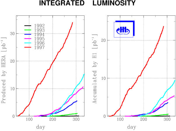
Abbildung 5.1: Integrated luminosity produced and accumulated during the running periods from $1992$ up to $1997$.

5.1 Background Sources

Nevertheless, it should be kept in mind that background processes are enhanced right along. In fact, interactions with atoms of the rest gas in the beam pipe are even dominating! Table 5.1 gives an impression of the rates to expect. Therefore, a careful consideration of possible background sources is necessary. Basically, they can be subdivided into “true” background not related to $ep$ collisions and misinterpreted competing $ep$ reactions. The first are common to all analyses, whereas the latter depend on the topic under study.

Cross sections and rates (at design luminosity)
Beam gas interactions		$50000\,{\rm Hz}$
Cosmic myons		$700\,{\rm Hz}$
Photoproduction	$1600\,{\rm nb}$	$25\,{\rm Hz}$
NC DIS, $Q^{2}<100\,{\rm GeV}^{2}$	$150\,{\rm nb}$	$2.2\,{\rm Hz}$
NC DIS, $Q^{2}>100\,{\rm GeV}^{2}$	$1.5\,{\rm nb}$	$0.022\,{\rm Hz}$
CC DIS, $P_{t}>25\,{\rm GeV}$	$0.05\,{\rm nb}$	$0.001\,{\rm Hz}$

Tabelle 5.1: Cross sections and rates at a design luminosity of $1.5\times 10^{31}\,{\rm cm}^{-2}{\rm s}^{-1}$ [8].

5.1.1 Non-$ep$ Background

Beam Gas Interactions

Instead of colliding with particles from the other beam, it is also possible (and even probable) to hit residual gas atoms. Especially the high energetic protons are able to produce large numbers of particles that may be scattered into the detector. Most of these events can be rejected because there is no vertex or the tracks point to vertices outside the interaction region.

Cosmic Myons

The surface of the earth and henceforth the detector are constantly hit by myons of cosmic origin. Most of them cross the experiment out of time with respect to $ep$ collisions and out of place, i.e. nowhere near the interaction region. Owing to their high rate, however, sometimes they pass in time right through the CTD and fake DIS events, despite the fact that they usually deposit little energy in the LAr. Still, they can be identified topologically by looking for back to back tracks in the IRON and CTD. In addition, the produced clusters are low energetic and imbalanced in transverse momentum.

Halo Myons

A second source of myons are stray protons interacting with material around the beam line. They always surround the proton beam (halo) and occasionally give rise to electromagnetic showers in the calorimeters, but since they are moving along the proton direction, they usually do not cause high $p_{t}$ tracks in the CJC.

5.1.2 $ep$ Background

Concerning our aim to investigate NC DIS, the following processes have to be considered as background.

Photoproduction

The term “photoproduction” derives from the picture of a quasi-real photon interacting with the proton, i.e. $Q^{2}\approx 0$. Hence, the electron is only slightly deflected from its original direction and escapes the central detectors. Instead, it can be found with a certain efficiency in the electron tagger of the luminosity system. Nevertheless, the $\gamma p$ reaction may result in a hadronic final state involving large transverse momenta. The misidentification of a particle as the scattered electron is then, due to the very high rate (s. table 5.1), a main source of background.

Diffractive Events

Another name for these reactions is “Large Rapidity Gap events” (LRG’s), where the rapidity is defined as

$$y_{R}:=\frac{1}{2}\ln\frac{E+p_{z}}{E-p_{z}}\,.$$ (5.3)

In the case of massless four-momenta, it is identical to the pseudo-rapidity

$$\eta:=-\ln\left(\tan\frac{\theta}{2}\right)\,.$$ (5.4)

In the region between the proton remnant and the current jet, which are normally connected via colour forces, an unusual gap without hadronic activity is exhibited. These events constitute around $5$–$10\%$ of the NC DIS sample, yet they are not described by the pQCD calculations invoked and have to be excluded.

CC Reactions

At last, it may happen that clusters of the hadronic final state in one of the seldom CC events with a neutrino as scattered lepton are misidentified as electron. Since the neutrino, however, escapes detection completely, the total transverse momentum is imbalanced.

5.2 Trigger Scheme

To keep notwithstanding the high rates the dead time of the experiment low and specifically select true $ep$ collisions, a trigger system has been set up in four stages [8]. The total read-out time of the detector of $\approx 1\,{\rm ms}$ is four orders of magnitude larger than that between two bunch-crossings of $\approx 0.1\mu{\rm s}$. Therefore, only a small part of the measured data, especially those from detector parts with short response times, is available for a fast decision.

The first level trigger L1 collects information from nine trigger systems attached to one subdetector each. These trigger elements are combined to form various subtriggers which provide a KEEP or REJECT signal within $2.5\,\mu{\rm s}$. A pipelining system stores the full data at the front end during the delay caused by L1 and ensures a dead time free running at this stage.

For future requirements intermediate trigger levels L2 and L3 are foreseen to operate during primary dead time of the read-out and are based on the same input as L1. However, they are able to evaluate a larger number of signals and their complex correlations. The decision times of these systems are designed to be around $20\,\mu{\rm s}$ and $800\,\mu{\rm s}$ respectively.

The last stage consists of the L4 software trigger, which has the raw data of the full event at its disposal. Depending on the time consumption, either fast algorithms specifically adapted to the requirements of L4 or parts of the standard offline reconstruction program H1REC [34] are applied to reach a quick decision. All events accepted by L4 are finally stored on tape. In addition, a small fraction of L4 ReJecTed events (L4RJT’s) of $\approx 1\%$ are kept for monitoring purposes.

The complete scheme including a fifth level L5 discussed in the next section is illustrated in fig. 5.2.

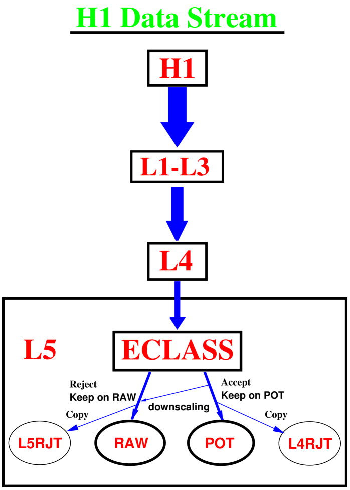
Abbildung 5.2: A principal diagram of the data stream in H1. Three levels of triggers operating with fast signals from nine detector branches and one software trigger evaluating the complete raw data are responsible for the rejection of background. A fifth level L5 works on fully reconstructed events and categorizes them into physics classes that are stored as POT’s. To avoid overflowing them, the classes may be downscaled. Events accepted by L4 but falling in no physics class at all are kept as raw data only. Small samples of L4 and L5 rejected data are retained for monitoring purposes.

5.3 Event Classification

Even after all four trigger stages, the reconstructed events kept for physics analysis contain to a large part unwanted or background reactions for most investigations. To save tape, network and computing resources, the program FPACK [35] used for platform independent data access has the possibility to skip events according to a classification word stored directly at the beginning of an event. Thereby, only the properly marked data tracks are completely read. Depending on the aim of a study, different classes, each matching to a set bit in the classification word, can be selected. Events falling in no physics class at all are L5 ReJecTed (L5RJT). They are kept as raw data, but do not appear fully reconstructed on Production Output Tapes (POT’s), except for a small fraction for monitoring purposes as in the case of L4RJT’s.

The chief requirement distinguishing NC DIS from background processes is the presence of a candidate for the scattered electron in the BEMC or LAr calorimeter. Therefore, loose criteria such as the existence of at least one compact mainly electromagnetic cluster with a minimal energy of several $\,{\rm GeV}$ are applied to define two DIS classes, a low $Q^{2}$ class (no. $11$) in case of the BEMC and a high $Q^{2}$ one (no. $9$) for the LAr.

Using additionally data from the tracking and myon systems, beam-induced and cosmic background is rejected more effectively.

5.4 Preselection

Due to the soft cuts applied in the event classification, the resulting classes are usually still too contaminated with background. In addition, some analyses might not need all parts of the intended content. Yet, physics studies are refined and iterated several times before being finished so it is recommendable to reduce the data sample further. This is done by a preselection which copies the selected events to a local disk for fast access.

Since the operation of such a complicated machinery like HERA and H1 is no easy task, running conditions are subject to variations. Any time a significant change in status like the (temporary) failure of an important detector component occurs, a new run is initiated. Only runs qualified as “medium” or “good” are allowed by the preselection. Additionally, the most important detector components for this analysis, i.e. the CJC1/2 and LAr for class $9$ and also the BEMC and BPC for class $11$, are required to be operational.

Relying on the fact that at least the scattered electron should cause a well measured track, the existence of a reconstructed vertex is mandatory.

As mentioned above, it is evident for NC DIS that finally a clear candidate for the scattered electron should be found. In distinction to the event classification, stricter cuts have to be fulfilled now. In H1 a program package for PHysics ANalysis (H1PHAN [36]) is available containing several algorithms for that purpose. Two of them, QFSELH/M and QESCAT, are applied. Both exploit the properties that the scattered electron should be isolated from the jet of the struck parton due to $p_{t}$-balance and that it deposits its energy in form of a compact electromagnetic shower mainly in the ECAL part of the LAr or in the BEMC.

In the case of QFSELH/M, some additional requirements are imposed on the found candidate. A cone of radius $0.5$ in azimuthal angle $\phi$ and pseudo-rapidity $\eta$ is drawn around the candidate. At most $5\%$ of its energy is allowed to be measured within this cone. Additionally, a matching track has to be found within $5{{}^{\circ}}$ for high $Q^{2}$. For electrons in the BEMC, a hit in the BPC with a maximal distance of $5\,{\rm cm}$ from the cluster center projected onto the BPC $(x,y)$-plane has to be measured and the cluster radius may not exceed $5\,{\rm cm}$.

For the purpose of the preselection, events are accepted if a candidate is determined either way. In the final analysis QFSELH/M is utilized for the low $Q^{2}$ sample and QESCAT for the high $Q^{2}$ events. A comparison revealed marginal differences between the two electron finders.

At last, a minimal energy of the candidate of $9\,{\rm GeV}$ is called for, and it is ensured that safe regions of the calorimeters are hit by cuts on the polar angle of $10{{}^{\circ}}<\theta<150{{}^{\circ}}$ for the LAr and $157{{}^{\circ}}<\theta<173{{}^{\circ}}$ for the BEMC respectively. Because the minimal $Q^{2}$ demanded later is $49\,{\rm GeV}^{2}$, a slightly smaller value of $45\,{\rm GeV}^{2}$, calculated according to eq. (3.11), has to be surpassed by the low $Q^{2}$ events.

5.5 Final Cut Scenario

Before the last selection is applied, an additional routine rejects residual events due to cosmic myons. Furthermore, there may be no photons detected in the PD.

In order to achieve a clean DIS sample, the final cuts have to take into account detector acceptances, efficiencies and resolutions as well as the diverse background sources described in section 5.1. The latter have already been suppressed to some extent in the selection procedure above. Additionally, possible constraints of the theoretical model to compare with have to be considered.

The final cuts are subdivided into two basic categories:

• Phase space cuts:
  Due to unavoidable limitations either of the experimental apparatus or the theoretical model, it is not possible to choose at will a phase space to investigate. Hence, common kinematic requirements have to be imposed on the data as well as on the theory.

• Data quality cuts:
  These are necessary to ensure that background is suppressed and the measurement is of good quality. Then, the data can be corrected for detector effects and may be compared to theoretical predictions.

First, the phase space cuts will be defined. For a quick overview see table 5.2.

Phase space cuts:

• low $Q^{2}$: $49<Q^{2}/\,{\rm GeV}^{2}<100$, high $Q^{2}$: $196<Q^{2}/\,{\rm GeV}^{2}<10000$:
  To examine the $Q$-dependence of the event shapes, all events are grouped into eight bins in $Q$: $7$–$8\,{\rm GeV}$, $8$–$10\,{\rm GeV}$, $14$–$16\,{\rm GeV}$, $16$–$20\,{\rm GeV}$, $20$–$30\,{\rm GeV}$, $30$–$50\,{\rm GeV}$, $50$–$70\,{\rm GeV}$ and $70$–$100\,{\rm GeV}$. Note that there is a gap from $10\,{\rm GeV}$ to $14\,{\rm GeV}$ which corresponds to the excluded transition region between the BEMC and LAr calorimeters. The lower bound of $7\,{\rm GeV}$ is motivated by the fact that an energy of $Q/2=3.5\,{\rm GeV}$ should be available in the CH of the Breit frame. For $Q>100\,{\rm GeV}$ there is not enough statistics at hand.
  In case of data, $Q^{2}$ is identified with $Q_{e}^{2}$ according to eq. (3.11).

• $0.05<y<0.8$:
  As explained in section 3.2, the electron method is not well suited for the reconstruction of $y$-values as low as $0.05$. Hence, these events are rejected. At high $y$, radiative corrections due to an additional real photon emission of the scattered electron (s. section 6.1.1) are enormous and have to be avoided.
  For data, $y$ is identified with $y_{e}$ according to eq. (3.10) down to $0.15$. Below that value, $y_{h}$ from eq. (3.12) is taken instead. Note that nevertheless $y_{e}>0.05$ is asked for.

• low $Q^{2}$: $E_{e^{\prime}}>14\,{\rm GeV}$, high $Q^{2}$: $E_{e^{\prime}}>11\,{\rm GeV}$:
  Lower limits on the electron energy are imposed for several reasons: First, the trigger efficiency is above $99\%$ [37, 13]. Moreover, there are numerous clusters of hadronic origin, e.g. pions, which are low energetic and may fake electrons, especially when the real one did not even hit the main detectors e.g. in photoproduction. At last, true leptons which lost a large part of their original energy due to radiative effects are excluded. Thereby, a good measurement of $E_{e^{\prime}}$ should be reached, which is most important for the boost into the Breit frame.

• low $Q^{2}$: $157{{}^{\circ}}<\theta_{e^{\prime}}<173{{}^{\circ}}$, high $Q^{2}$: $30{{}^{\circ}}<\theta_{e^{\prime}}<150{{}^{\circ}}$:
  These cuts reflect the coverage in polar angle of the BEMC and LAr calorimeters, although the upper limit of $173{{}^{\circ}}$ for the low $Q^{2}$ sample is redundant owing to $Q^{2}>49\,{\rm GeV}^{2}$. For the high $Q^{2}$ events, the forward region $\theta_{e^{\prime}}\leq 30{{}^{\circ}}$ with its high hadronic activity is left out to avoid misidentifications of the scattered electron.

• $20{{}^{\circ}}<\theta_{q}$:
  $\theta_{q}$, eq. (4.7), indicates the direction of the $-z^{\star}$-axis in the laboratory system. The requirement $\theta_{q}>20{{}^{\circ}}$ ensures a sufficient detector resolution in polar angle (s. the discussion in section 4.1.2). In the low $Q^{2}$ regime, this cut-off is automatically fulfilled owing to the previous selection in $Q^{2}$ and $y$; a small number of high $Q^{2}$ events, however, is discarded, cf. fig. 5.3.

• $\tau_{P}$, $B_{P}$, $\rho_{E}$, $\tau_{C}$ and $C_{P}$ only: $E^{\star}>Q/10$:
  As explained in section 4.2, this cut is essential to keep the event shapes $\tau_{P}$, $B_{P}$, $\rho_{E}$, $\tau_{C}$ and $C_{P}$ infrared safe. In this sense, it is part of their definition. Experimentally, it ensures a minimum of hadronic activity in the CH and suppresses events substantially influenced by noise and leakage out of the RH.

Phase space cuts
	low $Q^{2}$ sample (BEMC)	high $Q^{2}$ sample (LAr)
Cut • ‣ 5.5	$49\,{\rm GeV}^{2}<Q^{2}<100\,{\rm GeV}^{2}$	$196\,{\rm GeV}^{2}<Q^{2}<10000\,{\rm GeV}^{2}$
Cut • ‣ 5.5	$0.05<y<0.8$
Cut • ‣ 5.5	$E_{e^{\prime}}>14\,{\rm GeV}$	$E_{e^{\prime}}>11\,{\rm GeV}$
Cut • ‣ 5.5	$157{{}^{\circ}}<\theta_{e^{\prime}}<173{{}^{\circ}}$	$30{{}^{\circ}}<\theta_{e^{\prime}}<150{{}^{\circ}}$
Cut • ‣ 5.5	$20{{}^{\circ}}<\theta_{q}$
Cut • ‣ 5.5∗	$E^{\star}>Q/10$

Tabelle 5.2: Final phase space cuts. Note that the starred cut no. • ‣ 5.5 is applied for $\tau_{P}$, $B_{P}$, $\rho_{E}$, $\tau_{C}$ and $C_{P}$ only.

For an overview of the data quality cuts see table 5.3.

Data quality cuts:

• $\tau_{P}$, $B_{P}$, $\rho_{E}$, $\tau_{C}$ and $C_{P}$ only: $N_{\rm CH}\geq 2\,;\;(F-F_{\rm min})\,,(F_{\rm max}-F)>5\cdot 10^{-5}$:
  Asking for at least two objects in the CH, “unnatural” peaks at zero for $\rho_{E}$, $\tau_{C}$ and $C_{P}$ in the low $Q^{2}$ region are removed. “Unnatural” means that they are caused either by leakage out of the remnant fragmentation region or by cutting off “regular” jets just at the border between the two hemispheres. In fact, $B_{P}$ does exhibit a pronounced peak at $0.5$ for the rejected events showing the hadrons/clusters to have polar angles marginally larger than the required $90{{}^{\circ}}$ in the Breit frame. For the same reason, the extreme values $F_{\rm min}$ and $F_{\rm max}$ are excluded by very small cut-offs.

• $E_{\rm forw}>0.5\,{\rm GeV}$:
  Requiring a minimal energy deposition in the forward region defined by $4{{}^{\circ}}<\theta<15{{}^{\circ}}$, diffractive events not described by usual pQCD calculations are discarded.

• $5.7{{}^{\circ}}\leq\theta_{\rm cl}\leq 170{{}^{\circ}}$:
  This cut reflects the angular acceptance for clusters that are completely contained in the LAr or BEMC calorimeters.

• $30\,{\rm GeV}<(E-P_{z})<65\,{\rm GeV}$:
  If all emerging particles of an $ep$ reaction could be measured perfectly, then

  $$(E-P_{z}):=\sum_{i}(E_{i}-p_{z_{i}})$$ (5.5)

  would be $E_{p}-p_{z_{p}}+E_{e}-p_{z_{e}}=2\cdot E_{e}=55\,{\rm GeV}$. Losses due to limited acceptance, e.g. around the beam pipe, transform this peak into a broad distribution with tails down to very low values. Restricting the range of $(E-P_{z})$ effectively reduces the photoproduction background and the size of radiative corrections.

• low $Q^{2}$: $P_{t}<7.5\,{\rm GeV}$, high $Q^{2}$: $P_{t}<15\,{\rm GeV}$:
  The total transverse momentum

  $$P_{t}:=\sqrt{\left(\sum_{i}p_{x_{i}}\right)^{2}+\left(\sum_{i}p_{y_{i}}\right)^{2}}$$ (5.6)

  of a NC event should normally be zero. To suppress remaining background from CC reactions or badly measured events, maximal $P_{t}$’s of $7.5\,{\rm GeV}$ and $15\,{\rm GeV}$ are allowed in the low $Q^{2}$ and high $Q^{2}$ samples respectively.

• $\left|(E_{e^{\prime}}-E_{da})/E_{da}\right|<0.25$:
  According to

  $$E_{da}:=\frac{Q_{da}^{2}}{4E_{e}}+E_{e}(1-y_{da})\,,$$ (5.7)

  the energy of the scattered electron can be derived from angular information only. This fact is exploited e.g. for the energy calibration of the calorimeter. Asking for both values to be compatible within $\approx 3\sigma$ suppresses events strongly affected by QED radiation.

• $-35\,{\rm cm}<z_{\rm v}-\left<z_{\rm v}\right><35\,{\rm cm}$:
  Here, it is enforced that an interaction vertex could be determined which lies within $\pm 35\,{\rm cm}\approx 3\sigma$ around the average $z$-position for the corresponding run period. In $1994$, $\left<z_{\rm v}\right>\approx 3\,{\rm cm}$, and in $1995$–$1997$, $\left<z_{\rm v}\right>\approx-1\,{\rm cm}$.

• $E_{\rm backw}<10\,{\rm GeV}$:
  Due to the very limited capability of the BEMC calorimeter to measure hadronic energies, events with significant activity there are discarded. In addition, unidentified scattered electrons in the BEMC may lead to a rejection.

• LAr only: $\left|\phi_{\rm imp}-\phi_{\rm cr}\right|\geq 2{{}^{\circ}}$,
  $\neg\,(-65\,{\rm cm}<z_{\rm imp}<-55\,{\rm cm})\wedge\neg\,(15\,{\rm cm}<z_{\rm imp}<25\,{\rm cm})$:
  In order to ensure a reliable measurement of the scattered electron, partially inefficient regions such as cracks between calorimeter modules ($\phi$-cracks) or wheels ($z$-cracks) have to be avoided. $\phi_{\rm imp}$ and $z_{\rm imp}$ denote the impact coordinates of the electron.

Data quality cuts
	low $Q^{2}$ sample (BEMC)	high $Q^{2}$ sample (LAr)
Cut • ‣ 5.5∗	$N_{\rm CH}\geq 2\,,\quad F-F_{\rm min}>5\cdot 10^{-5}\,,\quad F_{\rm max}-F>5\cdot 10^{-5}$
Cut • ‣ 5.5	$E_{\rm forw}>0.5\,{\rm GeV}$
Cut • ‣ 5.5	$5.7{{}^{\circ}}\leq\theta_{\rm cl}\leq 170{{}^{\circ}}$
Cut • ‣ 5.5	$30\,{\rm GeV}<(E-P_{z})<65\,{\rm GeV}$
Cut • ‣ 5.5	$P_{t}<7.5\,{\rm GeV}$	$P_{t}<15\,{\rm GeV}$
Cut • ‣ 5.5	$\left|(E_{e^{\prime}}-E_{da})/E_{da}\right|<0.25$
Cut • ‣ 5.5	$-35\,{\rm cm}<z_{\rm v}-\left<z_{\rm v}\right><35\,{\rm cm}$
Cut • ‣ 5.5	$E_{\rm backw}<10\,{\rm GeV}$
Cut • ‣ 5.5		$\left|\phi_{\rm imp}-\phi_{\rm cr}\right|\geq 2{{}^{\circ}}$
		$\left|z_{\rm imp}-z_{\rm cr}\right|\geq 5\,{\rm cm}$

Tabelle 5.3: Final data quality cuts. Note that the starred cut no. • ‣ 5.5 is applied for $\tau_{P}$, $B_{P}$, $\rho_{E}$, $\tau_{C}$ and $C_{P}$ only. Depending on the theory to compare with, the cuts nos. • ‣ 5.5 and • ‣ 5.5 may have to be considered as phase space cuts, cf. the discussion in section 7.3.

The only considerable background remaining hereafter stems from photoproduction. In the low $Q^{2}$ sample it is estimated to be less than $3\%$, for the high $Q^{2}$ region it is negligible [23]. Residual radiative effects are accounted for by the correction procedure described in ch. 7.

To illustrate the stability of the described selection procedure, the number of events accumulated in 1994 for the low $Q^{2}$ as well as the high $Q^{2}$ sample is plotted versus the integrated luminosity ${\cal L}_{int}$ in fig. 5.4. Also demonstrated is the constancy of the number of events gathered per ${\cal L}_{int}$ of $\approx 1\,{\rm pb}^{-1}$ for all four years contributing to the high $Q^{2}$ sample. The term “pre-final” refers to the production of data n-tuples where additionally to the preselection the cosmic filter, the anti-photon tag and the cuts nos. • ‣ 5.5, • ‣ 5.5 and • ‣ 5.5 are in effect already. QFSELM/QESCAT is employed for the determination of the scattered electron. Statistics on the selection procedure can be looked up in table 5.4.

Abbildung 5.3: Distribution of finally selected events in the $(x,Q^{2})$-plane. For clarity, $1994$ data only are shown. The curves mark out the phase space cuts nos. • ‣ 5.5–• ‣ 5.5 in $y$, $E_{e^{\prime}}$, $\theta_{e^{\prime}}$ and $\theta_{q}$ as indicated; the cuts in $y$ correspond to the (unlabelled) dotted lines.

year	${\cal L}_{\rm int}/{\rm pb}^{-1}$	$\#$ preselected	$\#$ pre-final	$\#$ final
1994 high $Q^{2}$	$3.20$	$12177$	$9467$	$3646$
1995 high $Q^{2}$	$4.29$	$16199$	$12817$	$5006$
1996 high $Q^{2}$	$8.49$	$30319$	$23924$	$9478$
1997 high $Q^{2}$	$22.26$	$100466$	$61711$	$24477$
total high $Q^{2}$	$38.24$	$159161$	$107919$	$42607$
1994 low $Q^{2}$	$3.18$	$35051$	$24690$	$9761$

Tabelle 5.4: Integrated luminosities and events gathered in the selection steps.

\psfrag{L int * pb}{\boldmath${\cal L}_{\rm int}/{\rm pb}^{\scriptscriptstyle-1}$\unboldmath}\psfrag{Nr. of events}{No.\ of events}\psfrag{1994 lq}{\scriptsize{1994 low }\boldmath$Q^{2}$\unboldmath}\includegraphics{plotlumia94lq}

\psfrag{L int * pb}{\boldmath${\cal L}_{\rm int}/{\rm pb}^{\scriptscriptstyle-1}$\unboldmath}\psfrag{Nr. of events}{No.\ of events}\psfrag{1994 lq}{\scriptsize{1994 low }\boldmath$Q^{2}$\unboldmath}\psfrag{L int * pb}{\boldmath${\cal L}_{\rm int}/{\rm pb}^{\scriptscriptstyle-1}$\unboldmath}\psfrag{Nr. of events}{No.\ of events}\psfrag{1994 hq}{\scriptsize{1994 high }\boldmath$Q^{2}$\unboldmath}\includegraphics{plotlumia94hq}

\psfrag{L int * pb}{\boldmath${\cal L}_{\rm int}/{\rm pb}^{\scriptscriptstyle-1}$\unboldmath}\psfrag{Nr. of events}{No.\ of events}\psfrag{1994 lq}{\scriptsize{1994 low }\boldmath$Q^{2}$\unboldmath}\psfrag{L int * pb}{\boldmath${\cal L}_{\rm int}/{\rm pb}^{\scriptscriptstyle-1}$\unboldmath}\psfrag{Nr. of events}{No.\ of events}\psfrag{1994 hq}{\scriptsize{1994 high }\boldmath$Q^{2}$\unboldmath}\psfrag{L int * pb}{\boldmath${\cal L}_{\rm int}/{\rm pb}^{\scriptscriptstyle-1}$\unboldmath}\psfrag{Number of events/Lint/pb}{{No.\ of events}\boldmath$/{\cal L}_{\rm int}\,/{\rm pb}$\unboldmath}\includegraphics{lumiplot}

Abbildung 5.4: In the two plots on top, the accumulated events (upper curve: pre-final, lower curve: final) are drawn against ${\cal L}_{int}$ for the low and high $Q^{2}$ samples of 1994. A constant rate of incoming events is demonstrated. The lower plot presents the constancy of the number of events gathered per ${\cal L}_{int}$ of $\approx 1\,{\rm pb}^{-1}$ for all four years contributing to the high $Q^{2}$ sample. The statistical uncertainties are smaller than the marker sizes.

Kapitel 6 Event Simulation

Measurements with the H1 detector essentially comprise clusters, i.e. energy depositions in the calorimeters, and tracks in the tracking devices that are caused by long-lived particles, mainly hadrons. Yet, the objects dealt with in theoretical considerations of pQCD are partons or, equivalently, quarks, anti-quarks and gluons. Due to the complexity of the measuring apparatus and the underlying physical processes, a direct link from clusters and tracks backwards to hadrons or even partons can not be established. Nevertheless, information can be drawn from the selected data by comparing with model assumptions on a statistical basis. The first task to be carried out in this analysis chain consists in simulating the detector response to a given physics model. This simulation procedure is the subject of the next two sections.

6.1 Simulation

6.1.1 Parton Level

Starting with the calculation of the matrix element of the hard scattering to ${\cal O}(\alpha^{2}\alpha_{s})$, complicated integrals arise. For the purpose of generating “events,” they are solved by employing a Monte Carlo integration technique, s. e.g. [38]. Subsequently, the result has to be folded with pdfs describing the proton structure. For the purpose of easy access, the available sets of pdfs are compiled in the PDFLIB program library [39]. According to the probability distribution derived from the matrix element and the available phase space, a limited number of final state partons is “produced” within the framework of dedicated computer programs called Monte Carlo (MC) generators. For $ep$ DIS two such programs, LEPTO [40] and HERWIG [41], are available.

To account for higher orders in a Leading Logarithmic Approximation (LLA), both offer an implementation of Parton Showers (PS) including coherence effects. These branching algorithms may be attached to incoming (Initial State PS, ISPS) and outgoing partons (Final State PS, FSPS) as long as their four-momentum squared $t$ (virtuality) is above some adjustable threshold, typically around $t_{0}\approx 1$–$4\,{\rm GeV}^{2}$. Otherwise, the PS is terminated.

Alternatively, a Colour Dipole Model (CDM) can be invoked to describe gluon radiation including the first emission in the QCDC reaction. ARIADNE [42] supplies an implementation of the CDM, but is not intended to be a stand-alone program. Instead, it provides an interface to LEPTO so that it may be used within its framework.

Apart from ${\cal O}(\alpha_{s})$ QCD corrections to the Born cross section (3.21), also QED corrections of ${\cal O}(\alpha)$ may be sizable depending on the phase space. This is especially true for high $y$ and low $x$. Following the singularities proportional to $1/(k\cdot l^{\prime})$, $1/(k^{\prime}\cdot l^{\prime})$ and $1/(k-k^{\prime}-l^{\prime})^{2}$ that appear in the calculation of the real diagrams, they can instructively be labelled Initial State Radiation (ISR), Final State Radiation (FSR) and Compton contribution, where the latter plays only a minor role. Fig. 6.1 depicts the first two of them where the photons are radiated predominantly collinear to the incoming respectively outgoing lepton. Nevertheless, all three parts are defined in the whole phase space such that e.g. “ISR” photons may also be directed along the scattered lepton! In addition, this simple picture is only valid in LLA; beyond, the separation is not unique.

The event generator DJANGO [43] combines the abilities of LEPTO and HERACLES [44], which provides the QED radiative effects including virtual corrections due to 1-loop diagrams, into one software package offering the most complete description of $ep$ DIS events available.

Abbildung 6.1: ${\cal O}(\alpha)$ real corrections to the QPM Feynman graph fig. 3.3: ISR (left) and FSR (right) on the lepton side.

6.1.2 Hadron Level

Neglecting leptons and photons at this stage, we are left with partons of low virtualities $t\approx t_{0}$, where perturbation theory ceases to be applicable. Lacking better theoretical means, phenomenological models have to be invoked to perform the necessary fragmentation of partons into hadrons. Since the PS cut-off $t_{0}$ is an arbitrary parameter, the hadronization model should employ a similar scale from which to start in such a way that the dependence on $t_{0}$ largely cancels between the PS and the fragmentation process.

The two most popular models existing for this purpose are the string and the cluster fragmentation, both of which also consider colour coherence effects. The first one is implemented in JETSET [45], which is applied for this task by the MC generators of the last section except for HERWIG, which makes use of the second approach. Taking into account decays of unstable particles as well, the final outcome of this step consists of all particles traversing through a real detector.

6.1.3 Detector Simulation

So far the involved processes were of a basically theoretical nature and could be described by general purpose MC programs. Since now the detector response to the passing particles has to be reproduced, software specifically adapted to the measuring device is required. The software package employed by H1 is called H1SIM [46].

It is responsible for tracking the MC particles through a virtual H1 detector and simulating the response signals in detail. The “events” produced that way look like real data. For comparison purposes it is desirable to have as many MC events as possible, at least about the same amount as data are available. However, the simulation step is very time consuming and takes several seconds of computing time per event on the computer systems at disposal. Therefore, the MC models to use have to be chosen carefully.

6.2 Reconstruction

6.2.1 Cluster Level

Because the “raw” information (real and simulated) in the form of wire hits, cell voltages, etc. is not very intuitive with respect to the physics of $ep$ scattering, the data have to be refined. This reconstruction process is the task of another H1 software program, H1REC [34], which has to be identical for real and simulated events. As a result, it provides i.a. particle tracks and the calorimeter clusters extensively used in this study. For that reason, this stage is called “cluster level.”

6.3 Comparison to Data

Once the simulation and reconstruction have been completed, the MC models must be confronted with data. Ideally, they should give a good account of both, “standard” distributions where selection cuts are applied (the energy spectrum of the scattered electron, $dn/dE_{e^{\prime}}$, for example), as well as event shape distributions $dn/dF$ that are of special interest here.

In the previous publication [23], LEPTO 6.1 was shown to give the best description of the data. This is still true. However, it does not contain radiative corrections. Therefore, DJANGO 6.2 together with ARIADNE has been chosen as a replacement. In the following, the term “DJANGO 6.2” always refers to this combination!

For testing purposes a newer LEPTO version, LEPTO 6.5, and HERWIG 5.8 have been used. The basic differences to the old LEPTO version are changed default settings, a new cut-off scheme for the divergences of the matrix elements, an improved target remnant treatment and the introduction of soft colour interactions to facilitate the production of diffractive events within DIS samples. As will be seen, this has a considerable impact on the event shape distributions. Statistics of the employed MC files are given in table 6.1. In case of DJANGO 6.2 high $Q^{2}$, it should be noted that an extra very high $Q^{2}$ MC file was produced to increase the statistics in the $Q$-bins seven and eight. When combined with the other high $Q^{2}$ data sets, it would lead to unnatural steps in some of the distributions presented in the next section. Therefore, it was excluded there.

MC model	DJANGO 6.2	LEPTO 6.1	LEPTO 6.5	HERWIG 5.8
low $Q^{2}$ statistics	$4446$	$4253$	$-$	$-$
high $Q^{2}$ statistics	$121483$	$8906$	$84561$	$12617$

Tabelle 6.1: Cluster level MC statistics.

6.3.1 Standard Distributions

In figs. 6.3 and 6.4 the normalized differential distributions of $E_{e^{\prime}}$, $\theta_{e^{\prime}}$, $\ln(Q_{e}^{2}/\,{\rm GeV}^{2})$, $y_{h}$, $(E-P_{z})$ and $\theta_{q}$ are presented separately for the low $Q^{2}$ and high $Q^{2}$ sample. The comparison with DJANGO 6.2 as well as LEPTO 6.1 reveals a good overall agreement with the exception of low $\theta_{q}$-values in case of low $Q^{2}$ events. Yet, the imposed cut-off no. • ‣ 5.5 of $20{{}^{\circ}}<\theta_{q}$ is well below the smallest occurring angle of $\theta_{q,{\rm min}}\approx 30{{}^{\circ}}$, rendering the deviation harmless.

The dips in the high $Q^{2}$ $\theta_{e^{\prime}}$-distribution stem from the rejection of events with the scattered lepton found in areas of the LAr where the energy measurement deteriorates (cut no. • ‣ 5.5).

LEPTO 6.5 and HERWIG 5.8 are not shown here. Their agreement with data is similar.

6.3.2 Event Shape Distributions

The next step is to check the description of the event shape distributions. They are shown for four out of eight investigated bins in $Q$ in figs. 6.5 and 6.6. Here, the similarity is not as satisfactory as before. DJANGO 6.2 systematically tends to overshoot the data in the low $F$-region which is compensated for by underestimating them for high values in $F$. This is worst for $\tau_{P}$ and especially $B_{P}$, whose mean values come out too low in the MC. The uncorrected data means $\left<F\right>$ are given in table 6.2.

Within the much lower statistics available for LEPTO 6.1, it seems to do a better job in reproducing the data distributions. Nevertheless, DJANGO 6.2 in combination with ARIADNE provides an acceptable account of the available data and, since it includes radiative corrections, is employed for the primary correction procedure discussed in the next chapter.

As an example of a rather bad performance, fig. 6.2 presents the normalized differential distributions of $C_{P}$ for three bins of the high $Q^{2}$ sample in comparison with LEPTO 6.5 on the left-hand side and HERWIG 5.8 on the right-hand side. Severe deviations contrary to each other are observed.

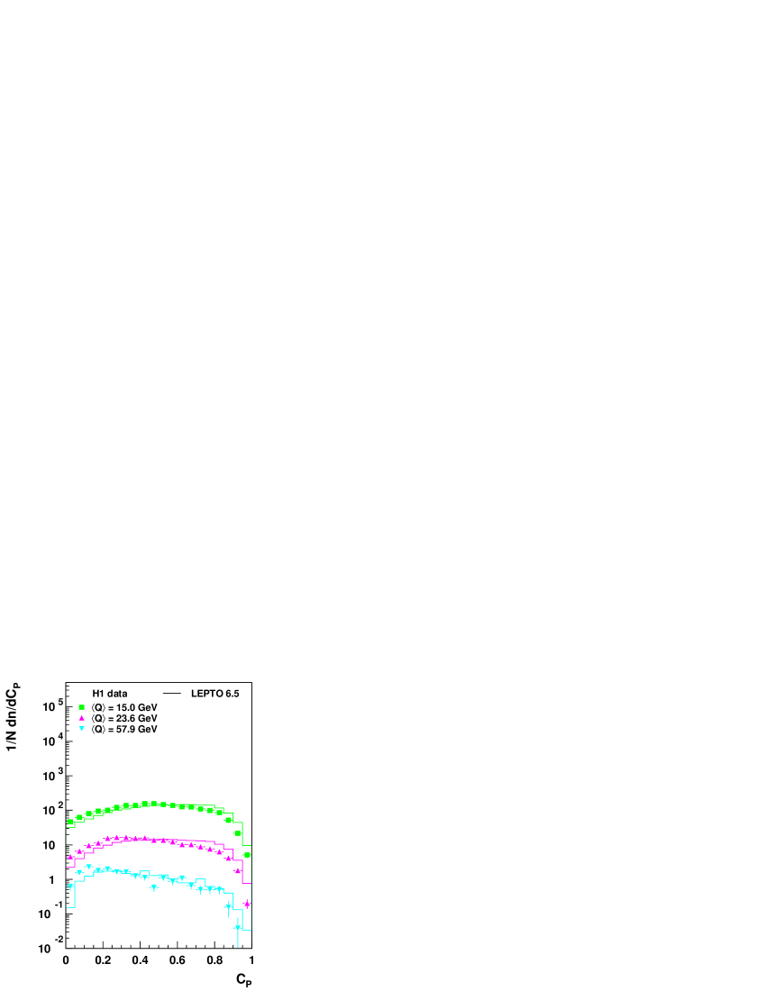
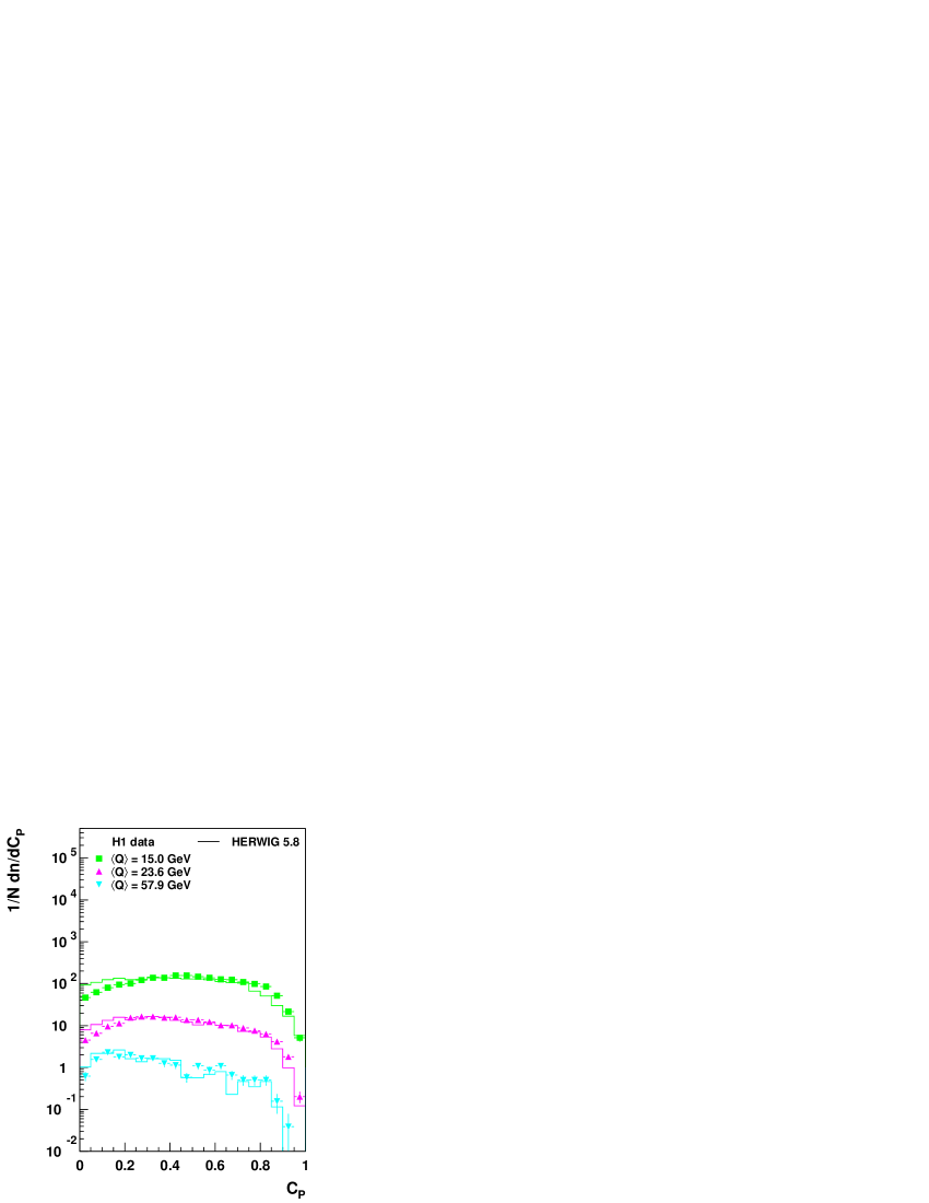
Abbildung 6.2: Normalized differential distributions of $C_{P}$ on cluster level. H1 data (full symbols) are compared with LEPTO 6.5 (full lines) on the left-hand side and HERWIG 5.8 (full lines) on the right-hand side for four out of eight investigated bins in $Q$. The spectra for $\left<Q\right>=7.5$–$57.9\,{\rm GeV}$ are multiplied by factors of $10^{n}$, $n=0,1,2,3$. The error bars represent statistical uncertainties only.

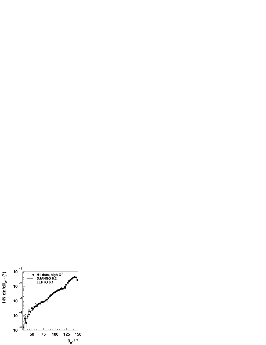
Abbildung 6.3: Normalized differential distributions of $E_{e^{\prime}}$, $\theta_{e^{\prime}}$ and $\ln(Q_{e}^{2}/\,{\rm GeV}^{2})$ on cluster level for the low $Q^{2}$ (left) and high $Q^{2}$ (right) data sample (full symbols) in comparison with DJANGO 6.2 (full line) and LEPTO 6.1 (dashed line). The error bars represent statistical uncertainties only.

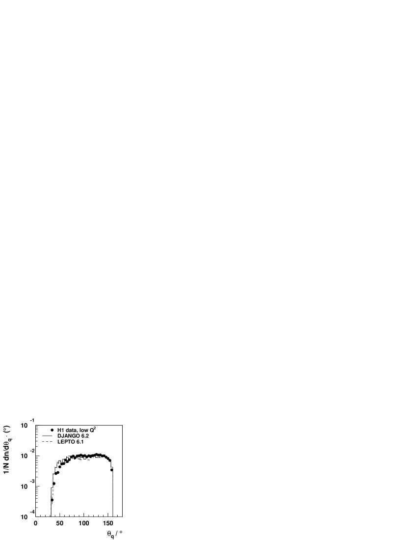
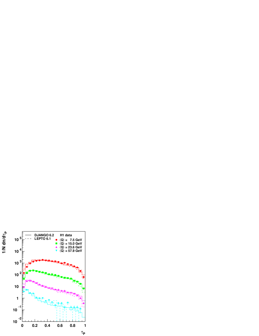
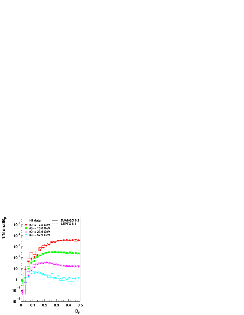
Abbildung 6.4: Normalized differential distributions of $y_{h}$, $(E-P_{z})$ and $\theta_{q}$ on cluster level for the low $Q^{2}$ (left) and high $Q^{2}$ (right) data sample (full symbols) in comparison with DJANGO 6.2 (full line) and LEPTO 6.1 (dashed line). The error bars represent statistical uncertainties only.

Abbildung 6.5: Normalized differential distributions of the event shapes $\tau_{P}$, $B_{P}$, $\rho_{E}$ and $\tau_{C}$ on cluster level. H1 data (full symbols) are compared with DJANGO 6.2 (full lines) and LEPTO 6.1 (dashed lines) for four out of eight investigated bins in $Q$. The spectra for $\left<Q\right>=7.5$–$57.9\,{\rm GeV}$ are multiplied by factors of $10^{n}$, $n=0,1,2,3$. The error bars represent statistical uncertainties only.

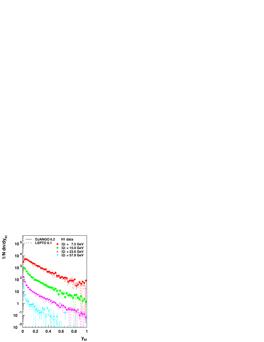
Abbildung 6.6: Normalized differential distributions of the event shapes $C_{P}$, $y_{fJ}$ and $y_{k_{t}}$ on cluster level. H1 data (full symbols) are compared with DJANGO 6.2 (full lines) and LEPTO 6.1 (dashed lines) for four out of eight investigated bins in $Q$. The spectra for $\left<Q\right>=7.5$–$57.9\,{\rm GeV}$ are multiplied by factors of $10^{n}$, $n=0,1,2,3$. The error bars represent statistical uncertainties only.

$\left<Q\right>/\,{\rm GeV}$	$\left<\tau_{P}\right>$	$\left<B_{P}\right>$
$7.46$	$0.4351\pm 0.0031$	$0.3651\pm 0.0013$
$8.74$	$0.4110\pm 0.0034$	$0.3543\pm 0.0014$
$14.97$	$0.3456\pm 0.0021$	$0.3186\pm 0.0010$
$17.75$	$0.3203\pm 0.0018$	$0.3039\pm 0.0009$
$23.62$	$0.2782\pm 0.0020$	$0.2790\pm 0.0010$
$36.72$	$0.2367\pm 0.0034$	$0.2502\pm 0.0019$
$57.93$	$0.2079\pm 0.0090$	$0.2271\pm 0.0053$
$81.32$	$0.1598\pm 0.0134$	$0.1891\pm 0.0082$

$\left<Q\right>/\,{\rm GeV}$	$\left<\rho_{E}\right>$	$\left<\tau_{C}\right>$	$\left<C_{P}\right>$
$7.46$	$0.0797\pm 0.0007$	$0.1401\pm 0.0013$	$0.4960\pm 0.0034$
$8.74$	$0.0805\pm 0.0008$	$0.1429\pm 0.0014$	$0.5048\pm 0.0038$
$14.97$	$0.0737\pm 0.0005$	$0.1297\pm 0.0008$	$0.4701\pm 0.0022$
$17.75$	$0.0725\pm 0.0004$	$0.1267\pm 0.0007$	$0.4603\pm 0.0019$
$23.62$	$0.0685\pm 0.0004$	$0.1179\pm 0.0008$	$0.4324\pm 0.0021$
$36.72$	$0.0626\pm 0.0008$	$0.1041\pm 0.0013$	$0.3847\pm 0.0036$
$57.93$	$0.0578\pm 0.0021$	$0.0950\pm 0.0033$	$0.3495\pm 0.0098$
$81.32$	$0.0482\pm 0.0030$	$0.0804\pm 0.0050$	$0.3041\pm 0.0147$

$\left<Q\right>/\,{\rm GeV}$	$\left<y_{fJ}\right>$	$\left<y_{k_{t}}\right>$
$7.46$	$0.1273\pm 0.0012$	$0.1746\pm 0.0023$
$8.74$	$0.1274\pm 0.0013$	$0.1471\pm 0.0023$
$14.97$	$0.1131\pm 0.0009$	$0.1077\pm 0.0013$
$17.75$	$0.1115\pm 0.0008$	$0.0975\pm 0.0011$
$23.62$	$0.1047\pm 0.0009$	$0.0826\pm 0.0012$
$36.72$	$0.0911\pm 0.0015$	$0.0603\pm 0.0018$
$57.93$	$0.0874\pm 0.0044$	$0.0483\pm 0.0040$
$81.32$	$0.0681\pm 0.0060$	$0.0341\pm 0.0050$

Tabelle 6.2: Uncorrected mean values of the event shapes and their statistical uncertainty as a function of $Q$.

Kapitel 7 Correction Procedure

After having established a sufficient description of data by MC models, the most important task remaining is disentangling the underlying physics from mere detector effects due to limited efficiencies and resolutions. Additionally, radiative corrections are taken into account.

In principle, it is feasible to do this in a one-step procedure. Compensating effects, however, may mislead to the conclusion that the corrections are small, even if indeed they are not. Moreover, one would like to identify the dominant influence. Another disadvantage is the complete neglect of migrations enforced by the lack of correlations.

For those reasons, the procedure applied here tries to differentiate between these contributions, and the unfolding of the data is correspondingly performed in two stages. The different correction methods available are explained in the next section.

7.1 Unfolding Methods

7.1.1 Factor Method

When only mean values do matter, the easiest thing to think of is to invoke one correction factor for each mean:

$$\left<F\right>_{\rm corr}=c_{\rm had/sim}\cdot\left<F\right>_{\rm dat}\,,\qquad\qquad c_{\rm had/sim}:=\frac{\left<F\right>_{\rm had}^{\rm MC}}{\left<F\right>_{\rm sim}^{\rm MC}}\,.$$ (7.1)

7.1.2 Bin-to-bin Correction

By applying eq. (7.1) not to the mean values alone, but to each bin $i$ of a differential distribution $F_{i}$,

$$F_{i,{\rm corr}}=c_{i,{\rm had/sim}}\cdot F_{i,{\rm dat}}\,,\qquad\qquad c_{i,{\rm had/sim}}:=\frac{\frac{1}{N_{\rm had}^{\rm MC}}F_{i,{\rm had}}^{\rm MC}}{\frac{1}{N_{\rm sim}^{\rm MC}}F_{i,{\rm sim}}^{\rm MC}}\,,$$ (7.2)

the factor method can easily be extended to unfold complete distributions which again can be reevaluated to give a corrected mean $\left<F\right>_{\rm corr}$.

As can be seen from eq. (7.2), however, this simple approach completely ignores the possibility of migrations from one bin $i$ on hadron level to another bin $j$ on cluster level. Depending on the quantity to deal with, this constitutes a severe disadvantage. A measure to improve the situation is to choose bin sizes in such a way that migrations are minimized.

7.1.3 Matrix Method

It is still better to take these migrations explicitly into consideration by employing a correction matrix $C_{ij}$:

$$F_{i,{\rm corr}}=\sum\limits_{j}C_{ij}F_{j,{\rm dat}}\,.$$ (7.3)

The matrix $C_{ij}$ can in principle be obtained from MC by inverting the transfer matrix $T_{ij}$ which transforms the “true” values $F_{i,{\rm had}}^{\rm MC}$ into the observed ones

$$F_{i,{\rm sim}}^{\rm MC}=\sum\limits_{j}T_{ij}F_{j,{\rm had}}^{\rm MC}\,.$$ (7.4)

In practice, however, the inversion leads to instabilities and oscillations unless extremely large MC statistics is available. Instead, we follow the strategy employed in [23] to define the correction matrix to be

$$C_{ij}:=\frac{\rho_{ij}}{\sum\limits_{k}\rho_{kj}}$$ (7.5)

where $\rho_{ij}$ represents a probability density derived from MC correlations as

$$F_{i,{\rm had}}^{\rm MC}=\sum\limits_{j}\rho_{ij}F_{j,{\rm sim}}^{\rm MC}\,.$$ (7.6)

As a drawback of this scheme, there may remain some model dependence which can be overcome by an iterative procedure.

7.1.4 Bayesian Unfolding

The last method employs a program developed in [47]. It exploits Bayes’ theorem on conditional probabilities to extract information from the observed distributions. To state it in a more general form, we label the fact of an event to have a “true” value $F_{\rm corr}$ allocated to bin $i$ as “cause” $C_{i}$ and the observed value $F_{\rm dat}$ in bin $j$ as “effect” $E_{j}$. Since in general the binning and also the domain of definition may be different, we have a number of $N_{C}$ causes and $N_{E}$ effects. Denoting further the initial probability for cause $C_{i}$ to happen with $P_{0}(C_{i})$ and the conditional probability for the effect $E_{j}$ to occur if $C_{i}$ has already taken place with $P(E_{j}|C_{i})$, Bayes’ theorem can be written as

$$P(C_{i}|E_{j})=\frac{P(E_{j}|C_{i})\cdot P_{0}(C_{i})}{\sum\limits_{k=1}^{N_{C}}P(E_{j}|C_{k})\cdot P_{0}(C_{k})}\,.$$ (7.7)

That is, given an observation of $E_{j}$, we get a probability that it was produced by cause $C_{i}$.

The result, however, depends on two ingredients: the conditional probabilities $P(E_{j}|C_{i})$, which can be estimated from MC, and the initial probabilities $P_{0}(C_{i})$, that are a priori unknown. At first, the latter have to be assumed by the observer according to his prejudices which may even result in a uniform distribution in the case of complete ignorance. But, given a number of experimental observations with frequencies $N(E):=\{N(E_{1}),\ldots,N(E_{N_{E}})\}$, Bayes’ theorem can then be applied to gain information on $P_{0}(C_{i})$. Based on these observed event numbers for the effects $E_{j}$, the expected number of events to be assigned to the different causes $C_{i}$ can be inferred to be

$$\hat{N}(C_{i})=\sum\limits_{j=1}^{N_{E}}P(C_{i}|E_{j})\cdot N(E_{j})\,.$$ (7.8)

Ignoring the possibility of inefficiencies, i.e. the case when a cause does not produce one of the effects under consideration, the initial probability is estimated by

$$\hat{P}(C_{i}):=P(C_{i}|N(E))=\frac{\hat{N}(C_{i})}{\sum\limits_{i=1}^{N_{C}}\hat{N}(C_{i})}\,.$$ (7.9)

If the initial distribution $P_{0}(C_{i})$ is not consistent with the data, it will in general differ from the final one $\hat{P}(C_{i})$. In an iterative procedure where the assumption on $P_{0}(C_{i})$ is updated in each step, the observed events $N(E)$ can now be exploited to unfold the “true” distribution $\hat{N}(C)$.

7.2 Correction for Detector Effects

The first step consists in deriving a correction to hadron level from the simulated DJANGO 6.2 MC files. Here, special care has to be taken when specifying what is meant by “hadron level” since there may be radiative photons. But we are interested in detector effects only. Thus, the main influence of these photons has to be accounted for in a later step. This is accomplished by first enforcing a limitation in acceptance according to cut no. • ‣ 5.5, thereby throwing away radiation collinear to the incoming lepton. Furthermore, with regard to the finite angular resolution of the LAr calorimeter, the scattered electron is redefined to be merged with radiative photons if they are closer in angle than $5{{}^{\circ}}$. This value is motivated by a study in [48]. As a consequence, the cuts nos. • ‣ 5.5–• ‣ 5.5 may reject events with respect to this “radiative” hadron level.

Now one is free to draw a connection between the cluster and hadron level of the simulation and apply this to the data according to the four unfolding schemes described. Note that the selection criteria nos. • ‣ 5.5–• ‣ 5.5 are imposed on the cluster level only such that they are accounted for in this first step.

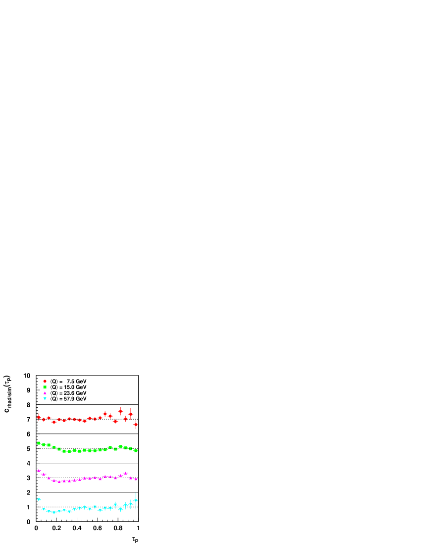
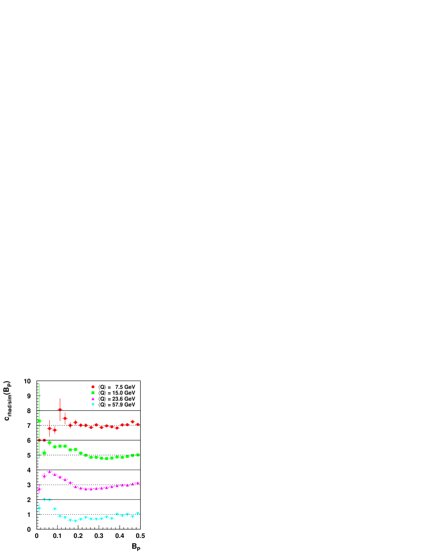
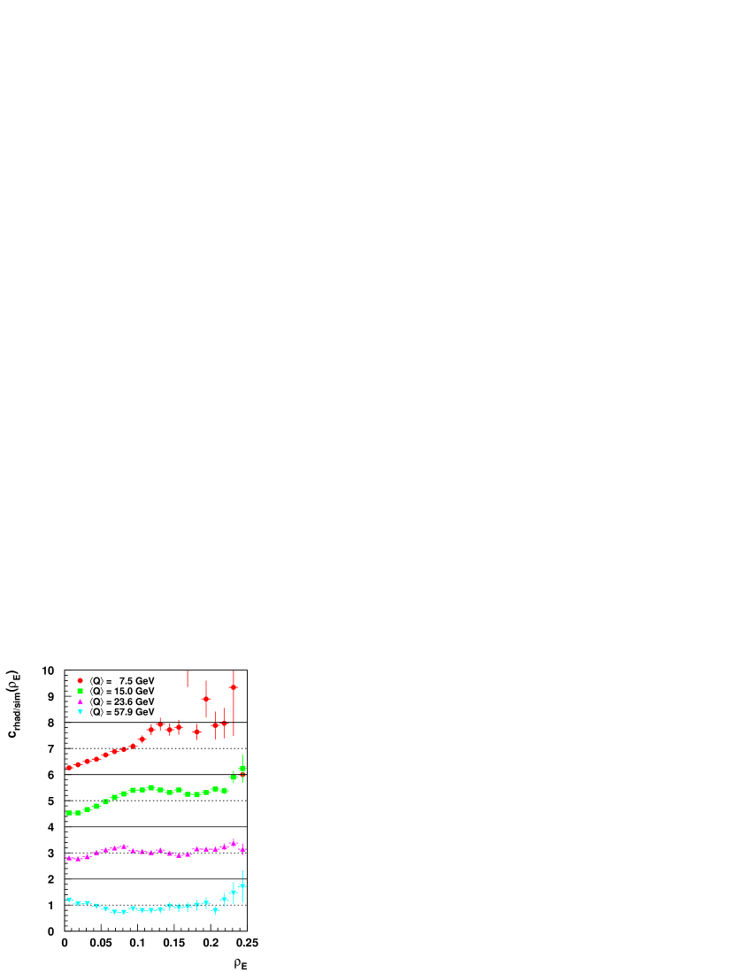
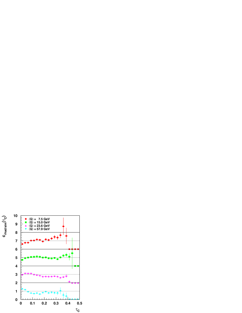
Abbildung 7.1: Bin-wise detector corrections for the event shapes $\tau_{P}$, $B_{P}$, $\rho_{E}$ and $\tau_{C}$ as derived from DJANGO 6.2 for four out of eight investigated bins in $Q$. The factors for $\left<Q\right>=7.5$–$57.9\,{\rm GeV}$ are shifted by offsets of $2\cdot n$, $n=0,1,2,3$. The dashed lines delineate the corresponding position of unity. Entries exactly at zero (or 2, 4, 6) mean that no events were found on either level. The error bars represent the statistical uncertainty.

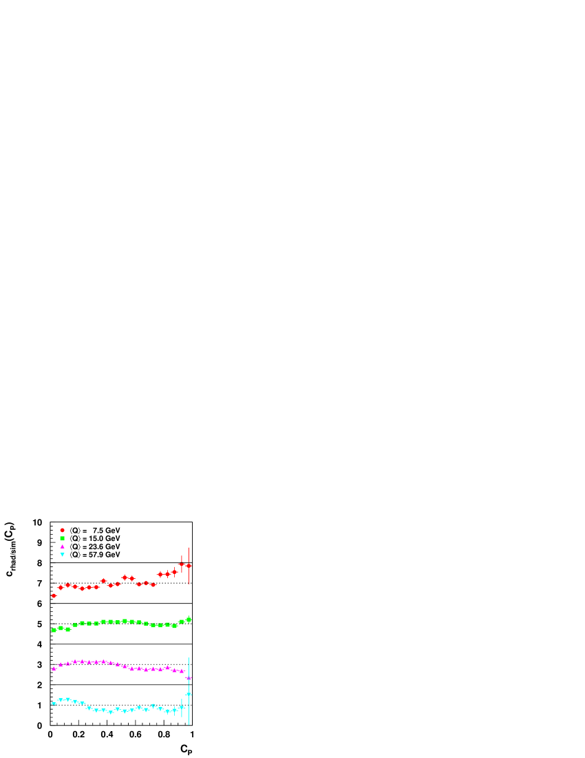
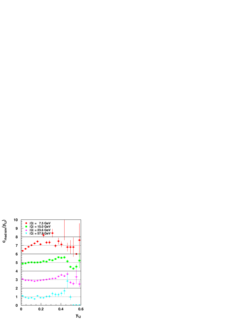
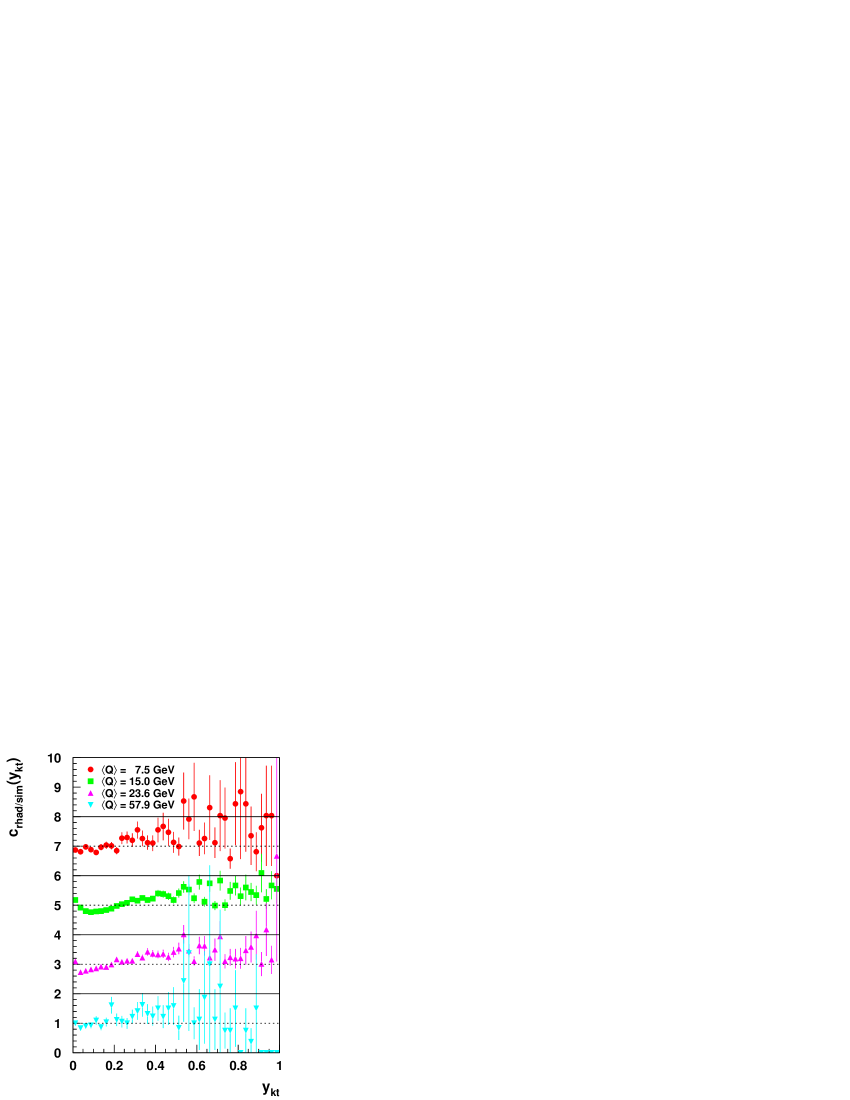
Abbildung 7.2: Bin-wise detector corrections for the event shapes $C_{P}$, $y_{fJ}$ and $y_{k_{t}}$ as derived from DJANGO 6.2 for four out of eight investigated bins in $Q$. The factors for $\left<Q\right>=7.5$–$57.9\,{\rm GeV}$ are shifted by offsets of $2\cdot n$, $n=0,1,2,3$. The dashed lines delineate the corresponding position of unity. Entries exactly at zero (or 2, 4, 6) mean that no events were found on either level. The error bars represent the statistical uncertainty.

Figs. 7.1 and 7.2 show the bin-wise detector corrections as derived from DJANGO 6.2 for four out of eight investigated bins in $Q$. Entries of zero (or correspondingly two, four or six) occurring at the edges mean that no events were found at either level. Concentrating on the statistically relevant points, it must be concluded that the corrections sometimes are larger than agreeable. Most often they are below $30\%$–$50\%$, but may rise higher in some bins, especially for $B_{P}$ and $\rho_{E}$.

Both, the matrix method as well as the Bayesian unfolding need the correlation matrices between hadron and cluster level as input. They are presented for each event shape in figs. 7.3–7.5 for two bins, one at low and one at high $Q^{2}$. Note that the box sizes are scaled logarithmically with the number of entries. From these we can learn mainly two things: First, correlations, which improve with rising $Q$, are clearly demonstrated, and second, with respect to the resolution, the bin sizes are too small for the bin-to-bin correction. Nevertheless, the binning is kept as a compromise, because the matrix and the Bayes unfolding account for migrations as well as resolution effects and the corrected means should not be affected by too coarse bin sizes.

With these ingredients given, two supplementary remarks are due. Concerning the matrix approach, the effect of iterations was revealed to be small, except for the fact that oscillations are gathered up. Hence, no iteration is performed here.

With respect to the Bayesian unfolding, it is recommended in [47] to avoid building up large fluctuations with an increasing number of iterations by smoothing a new “initial” distribution $\hat{P}(C_{i})$ in the intermediate steps. This proved to be difficult for the event shapes and finally was not done. To start from uniformly distributed initial probabilities did work, but required some iterations before converging, and consequently fluctuations showed up. It could be circumvented by choosing the MC distribution for $P_{0}(C_{i})$. Then, three iterations are fully sufficient.

7.3 Radiative Corrections

At this stage we have to perform the remaining correction from the previously defined radiative to a non-radiative hadron level. For that purpose a second kind of DJANGO 6.2 MC files is necessary. They have to be generated with exactly the same settings as the ones before, except for the radiative effects which have to be switched off. A simulation is not required. Because there are no more ISR or FSR photons, the acceptance cut no. • ‣ 5.5 may be dropped leaving the cuts nos. • ‣ 5.5–• ‣ 5.5 ineffective. In that way, the acceptance holes of the detector near the beam pipe are additionally compensated for. But due to our limited knowledge of that region, the extrapolation from MC possibly is not very precise. Notice that the cuts nos. • ‣ 5.5 and • ‣ 5.5 have been applied to all levels up to now and consequently they have not been accounted for by the unfolding procedure. Depending on the theory to compare with, e.g. the parton level of some MC, they may have to be considered as phase space cuts. Yet, they are not suitable in the framework of a pQCD calculation to NLO and hence are regarded as data quality cuts in this study.

For the factor and bin-to-bin method, the combined correction steps are fully equivalent to a one-step procedure. Yet, as a matter of fact, we now have to deal with two different MC files. That means we do not have any correlations at our disposal such that the unfolding schemes number three and four are not applicable. The bin-to-bin correction has to serve as the only available replacement.

Figs. 7.6 and 7.7 display the radiative correction factors for four out of eight investigated bins in $Q$. Except for $\tau_{P}$ and $B_{P}$ where radiative effects are not negligible, they are very close to one. $y_{k_{t}}$ is special. The additionally shown histogram with the full line usually near “one” corresponds to the correction factors where the acceptance cut no. • ‣ 5.5 was kept! This demonstrates that it is not a radiative effect. $y_{k_{t}}$ as applied here seems to be affected by the MC extrapolation, which is unfortunate and not understood at the moment. For all other event shapes including $y_{fJ}$, almost nothing changes whether cut no. • ‣ 5.5 is active or not. In the case of $\tau_{P}$ up to $C_{P}$ this could be expected since they only deal with the CH opposite to the remnant in the Breit frame.

7.4 Performance Check

A mandatory check of correction methods is to employ one MC to unfold another. As a first test, this was done for models without QED radiation. LEPTO 6.1 served as the MC, whereas LEPTO 6.5 and HERWIG 5.8 were treated like real data. Consequently, the unfolded means should predominantly lie close to the hadron level means of the corresponding MC (almost) regardless of what LEPTO 6.1 would prefer. To be able to discriminate between them, the models have to make sufficiently different predictions for the quantity under study. From fig. 6.2 it is clear that for $C_{P}$ this is certainly true. The outcome is presented in the upper plots of fig. 7.8 proving all four correction schemes to work properly. Nevertheless, all other event shapes were tested, too, yielding similar results, although not as evident.

In a second test, LEPTO 6.1 events were smuggled in as data for DJANGO 6.2. Here, the additional complication arises that the latter does include radiative effects in contrast to the “data.”  As expected, the first correction step alone suffices since the radiative hadron level is designed to separate detector and radiative effects as much as possible. If the radiative factors are applied, too, then the sensible variables, i.e. $\tau_{P}$ and $B_{P}$, are even overdone with. This is demonstrated in the lower plots of fig. 7.8, where the “fully” corrected means of the right plot deviate considerably from the hadron level means of LEPTO 6.1 as opposed to the plot on the left-hand side. Using only DJANGO 6.2 events without radiative photons, the discrepancy disappeared.

Concluding, it can be stated that the unfolding works satisfactorily.

Abbildung 7.3: Correlation matrices for the event shapes $\tau_{P}$, $B_{P}$ and $\rho_{E}$ as derived from DJANGO 6.2 for two out of eight investigated bins in $Q$. Note that the box sizes are scaled logarithmically with the number of entries.

Abbildung 7.4: Correlation matrices for the event shapes $\tau_{C}$, $C_{P}$ and $y_{fJ}$ as derived from DJANGO 6.2 for two out of eight investigated bins in $Q$. Note that the box sizes are scaled logarithmically with the number of entries.

Abbildung 7.5: Correlation matrices for the event shape $y_{k_{t}}$ as derived from DJANGO 6.2 for two out of eight investigated bins in $Q$. Note that the box sizes are scaled logarithmically with the number of entries.

7.5 Final Means

To illustrate possible systematic effects due to the different unfolding schemes, all resulting corrected means are shown in figs. 7.9 and 7.10. The statistical uncertainties encompass data as well as MC statistics. For the factor method, they are obtained properly by error propagation. In case of an evaluation from unfolded distributions, they are estimated by

$$\Delta\left<F\right>=\sigma(\left<F\right>)\cdot\left(\frac{1}{\sqrt{N_{\rm dat}}}+\frac{1}{\sqrt{N_{\rm MC}}}\right)\,,$$ (7.10)

where $N_{\rm dat}$, $N_{\rm MC}$ are the appropriate event numbers and $\sigma$ denotes the standard deviation. Note that $1/\sqrt{N_{\rm dat}}$ and $1/\sqrt{N_{\rm MC}}$ are not added conventionally in quadrature. This is motivated by the fact that the uncertainties derived this way are closer in value to those calculated for the factor method.

For the final results the differential distributions as well as the central values are taken from the most sophisticated approach, i.e. the Bayesian unfolding with subsequent bin-to-bin radiative correction. In case of the event shape spectra, no further error evaluation beyond statistical ones was attempted. For a comparison with pQCD calculations, their presentation is postponed to ch. 10, figs. 10.1 and 10.2.

Concerning the mean values, the other methods serve to judge systematic effects. The due asymmetric uncertainty is estimated to be half of the spread caused by the maximal deviation to larger respectively smaller values. The sum of both then corresponds to half the total spread which is somewhat smaller than $2/\sqrt{12}=1/\sqrt{3}$ as appropriate for a uniform distribution.

A second source of systematic uncertainties are the electromagnetic and hadronic energy scales of the calorimeters. Due to recent improvements [13], the electron energies now can be measured to a precision of $1\%$, $2\%$ and $3\%$ up to $z_{\rm imp}$-coordinates of $24\,{\rm cm}$, $110\,{\rm cm}$ and the forward end of the LAr calorimeter respectively. Hadronic energies are known only to about $4\%$. In order to gain information on the influence of this uncertainty, the whole analysis is repeated scaling up and down separately for both scales. The discrepancies with respect to the normal central values are then attributed to two further asymmetric systematic uncertainties. All three, i.e. including the unfolding, added in quadrature, yield the total systematics given together with the final results in table 7.1.

Concerning individual contributions, the impact of the electron energy, which directly affects the boost into the Breit frame, is almost always largest for $\tau_{P}$ up to $C_{P}$, followed by unfolding effects. Realizing that hadronic systematics cancel between numerator and denominator for these event shapes, this is understandable. The situation is reversed for $y_{fJ}$ and $y_{k_{t}}$. Here, no cancellation occurs and the systematic uncertainty due to hadronic energies dominates.

At last, figs. 7.11 and 7.12 present the final means including all uncertainties as well as the hadron level means of DJANGO 6.2 and LEPTO 6.1. Where available, already published results from [23] and [49] are shown for comparison. $\tau_{P}$ and $B_{P}$ are in good agreement, but they should not because radiative corrections leading to smaller values were previously neglected. Seemingly, this was compensated by an overestimation of the electron energy that happened before the new calibration was introduced into the analysis. Since $\rho_{E}$ and $\tau_{C}$ are much less affected by QED radiation, the new data are shifted somewhat towards higher means.

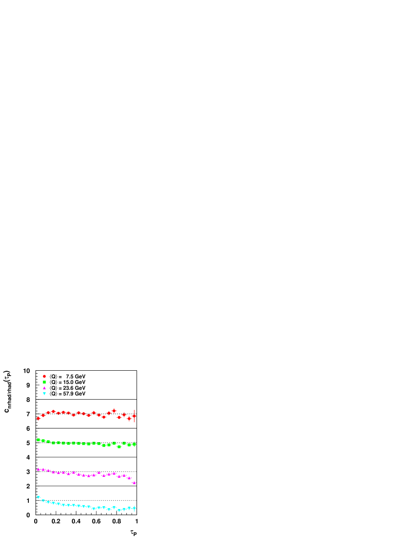
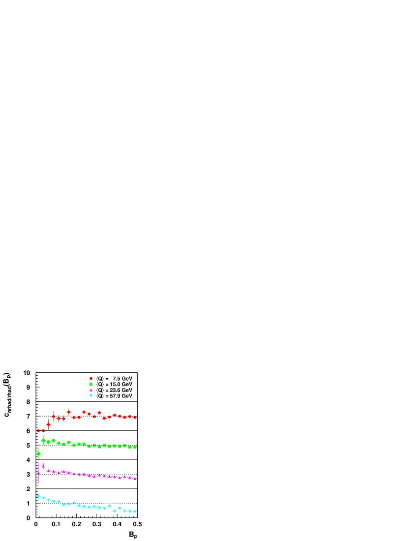
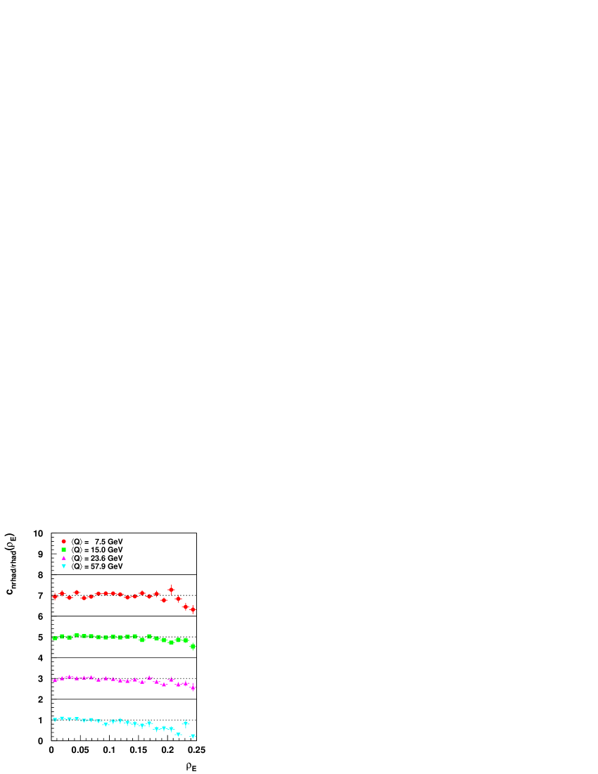
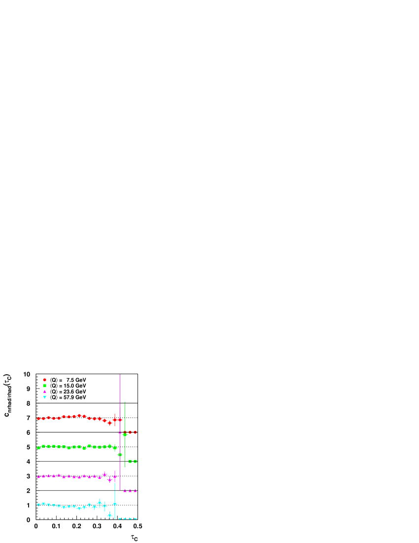
Abbildung 7.6: Bin-wise radiative corrections for the event shapes $\tau_{P}$, $B_{P}$, $\rho_{E}$ and $\tau_{C}$ as derived from DJANGO 6.2 for four out of eight investigated bins in $Q$. The factors for $\left<Q\right>=7.5$–$57.9\,{\rm GeV}$ are shifted by offsets of $2\cdot n$, $n=0,1,2,3$. The dashed lines delineate the corresponding position of unity. Entries exactly at zero (or 2, 4, 6) mean that no events were found on either level. The error bars represent the statistical uncertainty.

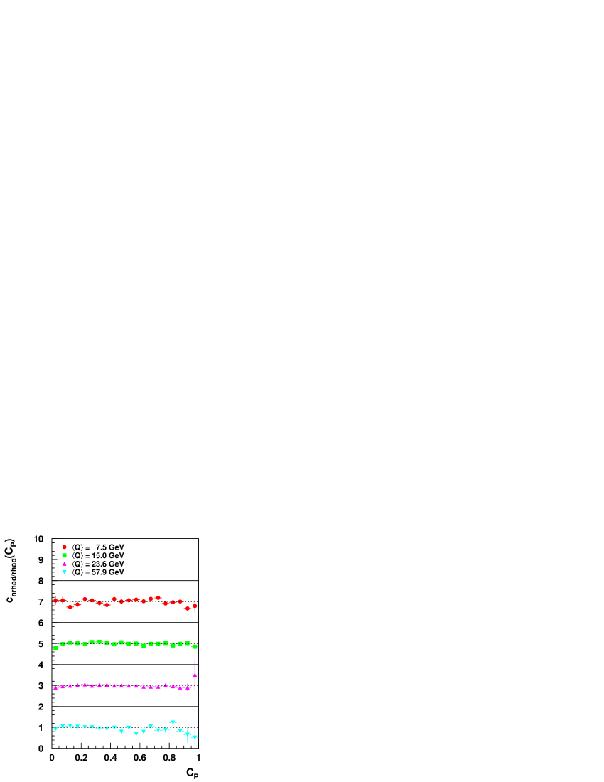
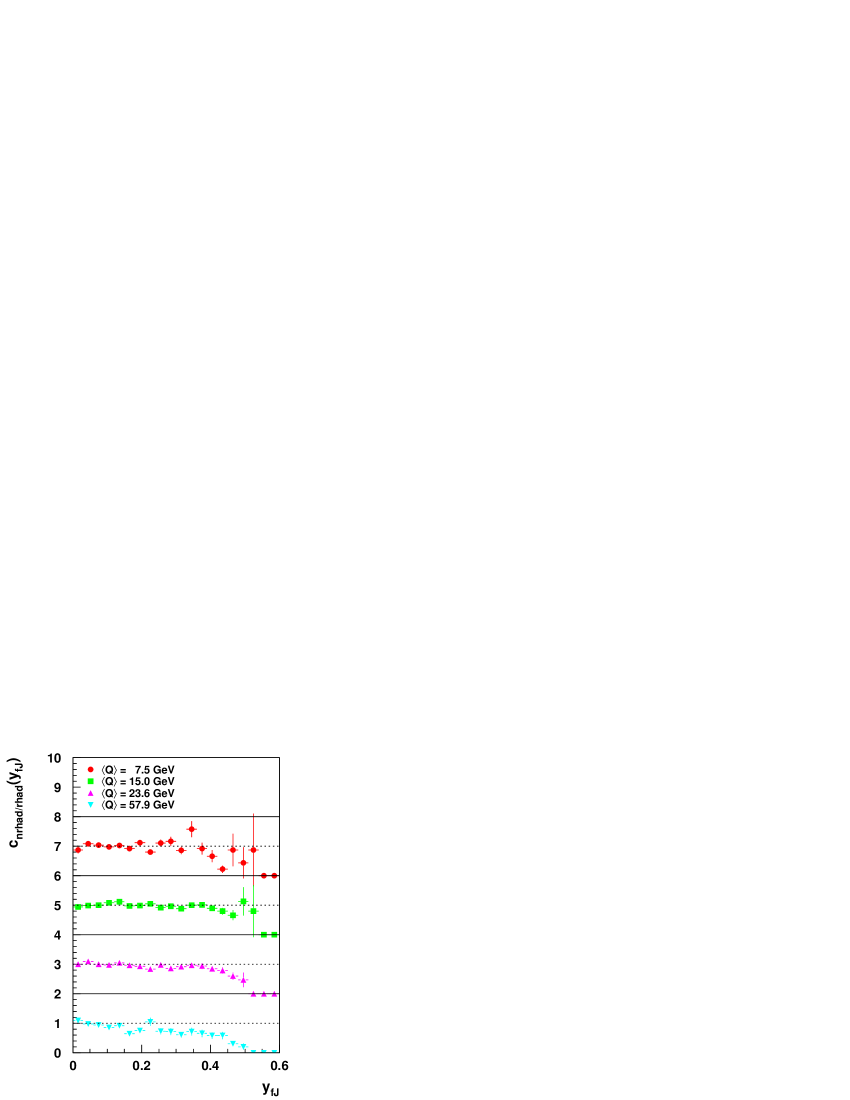
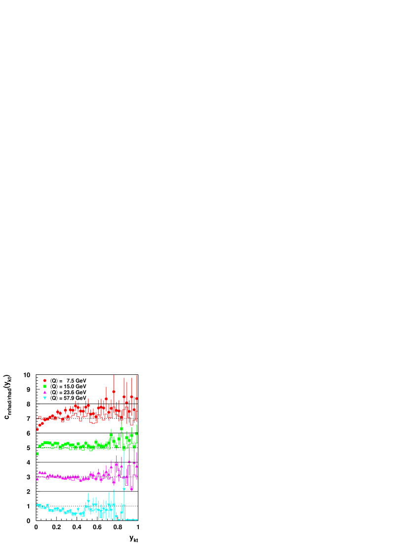
Abbildung 7.7: Bin-wise radiative corrections for the event shapes $C_{P}$, $y_{fJ}$ and $y_{k_{t}}$ as derived from DJANGO 6.2 for four out of eight investigated bins in $Q$. The factors for $\left<Q\right>=7.5$–$57.9\,{\rm GeV}$ are shifted by offsets of $2\cdot n$, $n=0,1,2,3$. The dashed lines delineate the corresponding position of unity. Entries exactly at zero (or 2, 4, 6) mean that no events were found on either level. The error bars represent the statistical uncertainty. For $y_{k_{t}}$ the additional histogram (full line) shows the correction factor without acceptance extrapolation.

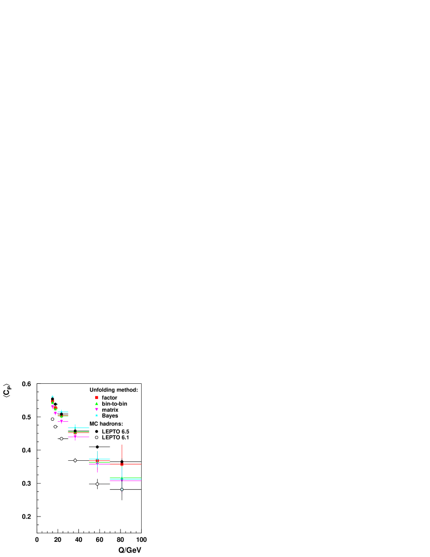
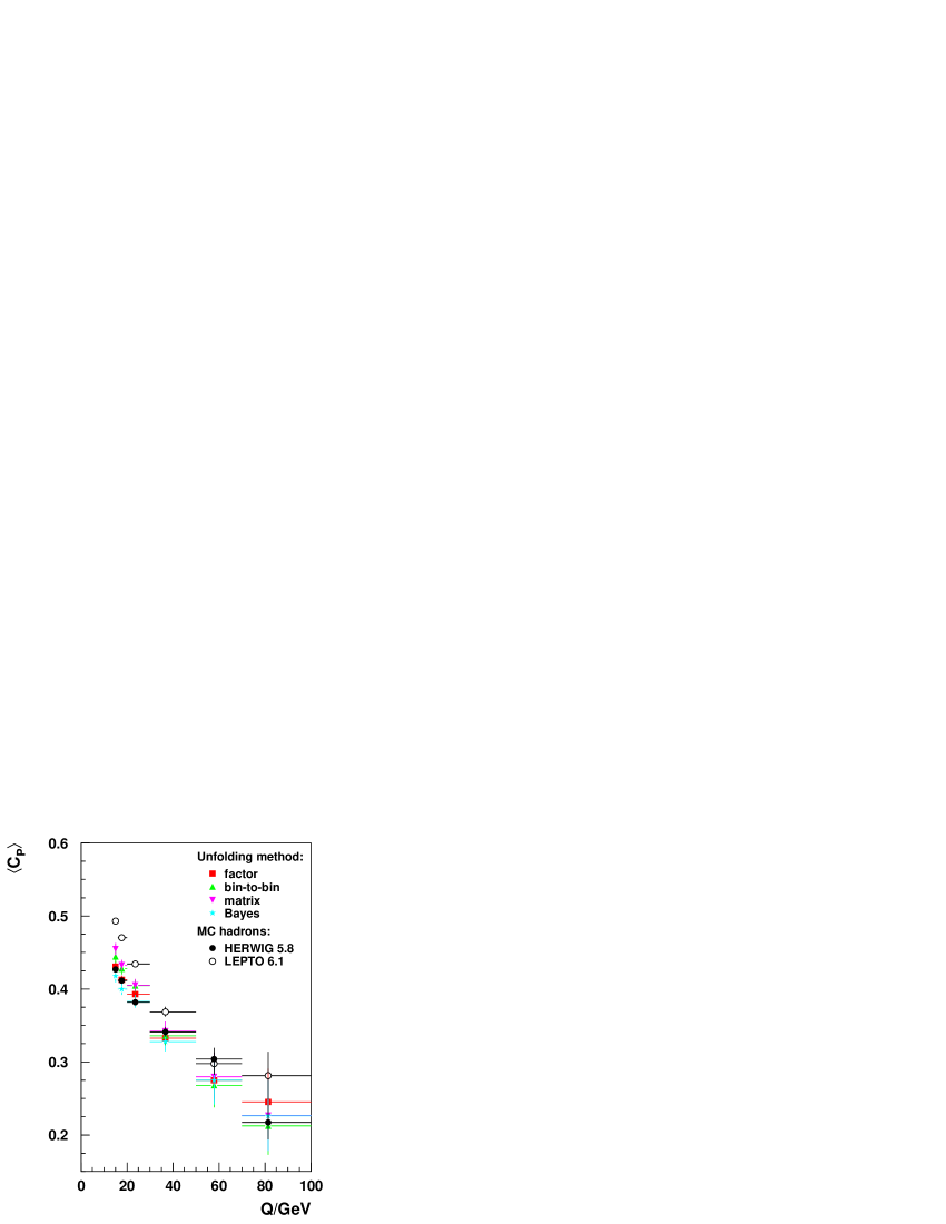
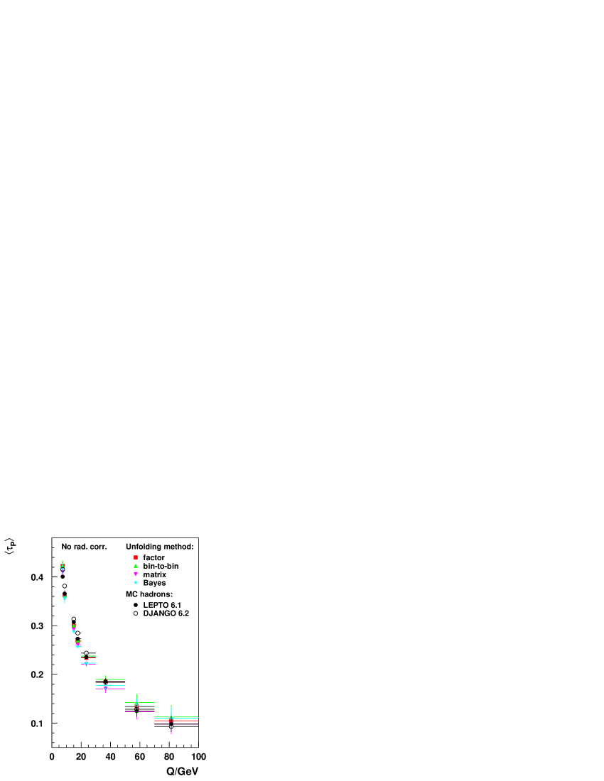
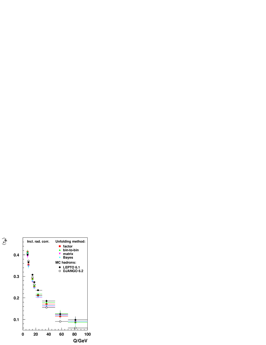
Abbildung 7.8: Top: Unfolded means of $C_{P}$ as a function of $Q$ for simulated high $Q^{2}$ LEPTO 6.5 (left) and HERWIG 5.8 (right) event samples. LEPTO 6.1 was employed as unfolding MC. Bottom: Unfolded means of $\tau_{P}$ as a function of $Q$ for simulated LEPTO 6.1 event samples with (right) and without (left) radiative corrections derived from DJANGO 6.2. In addition, the corresponding hadron levels of the MC’s are shown. The error bars represent statistical uncertainties only.

$\rule[-8.61108pt]{0.0pt}{21.52771pt}\left<Q\right>/\,{\rm GeV}$	$\left<\tau_{P}\right>$	$\left<B_{P}\right>$
$7.46$	$0.4402\pm 0.0082\leavevmode\nobreak\ ^{+0.0111}_{-0.0122}$	$0.3624\pm 0.0034\leavevmode\nobreak\ ^{+0.0046}_{-0.0038}$
$8.74$	$0.4017\pm 0.0090\leavevmode\nobreak\ ^{+0.0196}_{-0.0080}$	$0.3435\pm 0.0040\leavevmode\nobreak\ ^{+0.0076}_{-0.0037}$
$14.97$	$0.3052\pm 0.0034\leavevmode\nobreak\ ^{+0.0081}_{-0.0075}$	$0.2921\pm 0.0017\leavevmode\nobreak\ ^{+0.0044}_{-0.0033}$
$17.75$	$0.2762\pm 0.0029\leavevmode\nobreak\ ^{+0.0091}_{-0.0059}$	$0.2760\pm 0.0016\leavevmode\nobreak\ ^{+0.0054}_{-0.0034}$
$23.62$	$0.2279\pm 0.0031\leavevmode\nobreak\ ^{+0.0125}_{-0.0071}$	$0.2452\pm 0.0018\leavevmode\nobreak\ ^{+0.0078}_{-0.0042}$
$36.72$	$0.1814\pm 0.0049\leavevmode\nobreak\ ^{+0.0107}_{-0.0065}$	$0.2094\pm 0.0031\leavevmode\nobreak\ ^{+0.0083}_{-0.0053}$
$57.93$	$0.1330\pm 0.0089\leavevmode\nobreak\ ^{+0.0092}_{-0.0092}$	$0.1717\pm 0.0062\leavevmode\nobreak\ ^{+0.0109}_{-0.0096}$
$81.32$	$0.0984\pm 0.0130\leavevmode\nobreak\ ^{+0.0045}_{-0.0051}$	$0.1346\pm 0.0088\leavevmode\nobreak\ ^{+0.0117}_{-0.0041}$

$\rule[-8.61108pt]{0.0pt}{21.52771pt}\left<Q\right>/\,{\rm GeV}$	$\left<\rho_{E}\right>$	$\left<\tau_{C}\right>$	$\left<C_{P}\right>$
$7.46$	$0.1115\pm 0.0019\leavevmode\nobreak\ ^{+0.0011}_{-0.0013}$	$0.1637\pm 0.0032\leavevmode\nobreak\ ^{+0.0030}_{-0.0029}$	$0.5601\pm 0.0082\leavevmode\nobreak\ ^{+0.0083}_{-0.0073}$
$8.74$	$0.1044\pm 0.0021\leavevmode\nobreak\ ^{+0.0017}_{-0.0000}$	$0.1600\pm 0.0037\leavevmode\nobreak\ ^{+0.0060}_{-0.0031}$	$0.5524\pm 0.0094\leavevmode\nobreak\ ^{+0.0074}_{-0.0054}$
$14.97$	$0.0872\pm 0.0007\leavevmode\nobreak\ ^{+0.0007}_{-0.0014}$	$0.1333\pm 0.0013\leavevmode\nobreak\ ^{+0.0013}_{-0.0019}$	$0.4824\pm 0.0034\leavevmode\nobreak\ ^{+0.0036}_{-0.0051}$
$17.75$	$0.0826\pm 0.0007\leavevmode\nobreak\ ^{+0.0013}_{-0.0015}$	$0.1263\pm 0.0011\leavevmode\nobreak\ ^{+0.0014}_{-0.0024}$	$0.4621\pm 0.0030\leavevmode\nobreak\ ^{+0.0045}_{-0.0069}$
$23.62$	$0.0714\pm 0.0007\leavevmode\nobreak\ ^{+0.0019}_{-0.0016}$	$0.1098\pm 0.0012\leavevmode\nobreak\ ^{+0.0020}_{-0.0026}$	$0.4112\pm 0.0033\leavevmode\nobreak\ ^{+0.0056}_{-0.0076}$
$36.72$	$0.0634\pm 0.0012\leavevmode\nobreak\ ^{+0.0013}_{-0.0013}$	$0.0985\pm 0.0021\leavevmode\nobreak\ ^{+0.0012}_{-0.0023}$	$0.3644\pm 0.0058\leavevmode\nobreak\ ^{+0.0029}_{-0.0058}$
$57.93$	$0.0518\pm 0.0023\leavevmode\nobreak\ ^{+0.0016}_{-0.0025}$	$0.0834\pm 0.0040\leavevmode\nobreak\ ^{+0.0015}_{-0.0046}$	$0.3127\pm 0.0122\leavevmode\nobreak\ ^{+0.0065}_{-0.0131}$
$81.32$	$0.0410\pm 0.0034\leavevmode\nobreak\ ^{+0.0022}_{-0.0016}$	$0.0663\pm 0.0057\leavevmode\nobreak\ ^{+0.0031}_{-0.0025}$	$0.2529\pm 0.0173\leavevmode\nobreak\ ^{+0.0160}_{-0.0065}$

$\rule[-8.61108pt]{0.0pt}{21.52771pt}\left<Q\right>/\,{\rm GeV}$	$\left<y_{fJ}\right>$	$\left<y_{k_{t}}\right>$
$7.46$	$0.1554\pm 0.0031\leavevmode\nobreak\ ^{+0.0052}_{-0.0057}$	$0.2814\pm 0.0077\leavevmode\nobreak\ ^{+0.0072}_{-0.0123}$
$8.74$	$0.1399\pm 0.0034\leavevmode\nobreak\ ^{+0.0056}_{-0.0048}$	$0.2196\pm 0.0078\leavevmode\nobreak\ ^{+0.0109}_{-0.0088}$
$14.97$	$0.1226\pm 0.0014\leavevmode\nobreak\ ^{+0.0053}_{-0.0047}$	$0.1364\pm 0.0026\leavevmode\nobreak\ ^{+0.0080}_{-0.0071}$
$17.75$	$0.1164\pm 0.0014\leavevmode\nobreak\ ^{+0.0047}_{-0.0047}$	$0.1156\pm 0.0021\leavevmode\nobreak\ ^{+0.0068}_{-0.0061}$
$23.62$	$0.1015\pm 0.0015\leavevmode\nobreak\ ^{+0.0044}_{-0.0042}$	$0.0943\pm 0.0022\leavevmode\nobreak\ ^{+0.0059}_{-0.0041}$
$36.72$	$0.0898\pm 0.0026\leavevmode\nobreak\ ^{+0.0037}_{-0.0041}$	$0.0665\pm 0.0030\leavevmode\nobreak\ ^{+0.0041}_{-0.0015}$
$57.93$	$0.0752\pm 0.0050\leavevmode\nobreak\ ^{+0.0039}_{-0.0056}$	$0.0451\pm 0.0046\leavevmode\nobreak\ ^{+0.0064}_{-0.0024}$
$81.32$	$0.0557\pm 0.0063\leavevmode\nobreak\ ^{+0.0045}_{-0.0056}$	$0.0295\pm 0.0042\leavevmode\nobreak\ ^{+0.0046}_{-0.0028}$

Tabelle 7.1: Corrected mean values of the event shapes as a function of $Q$. The first error is statistical, the second systematic and comprises unfolding as well as energy scale uncertainties added quadratically.

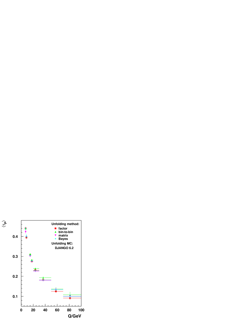
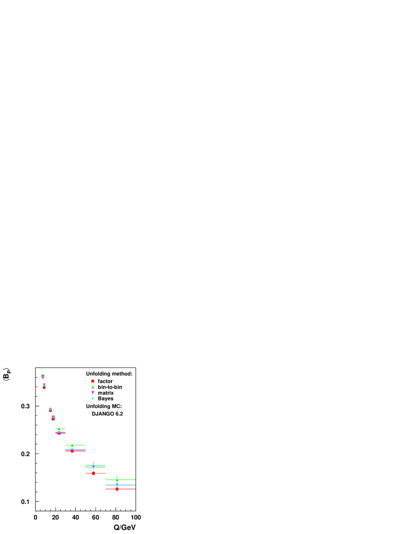
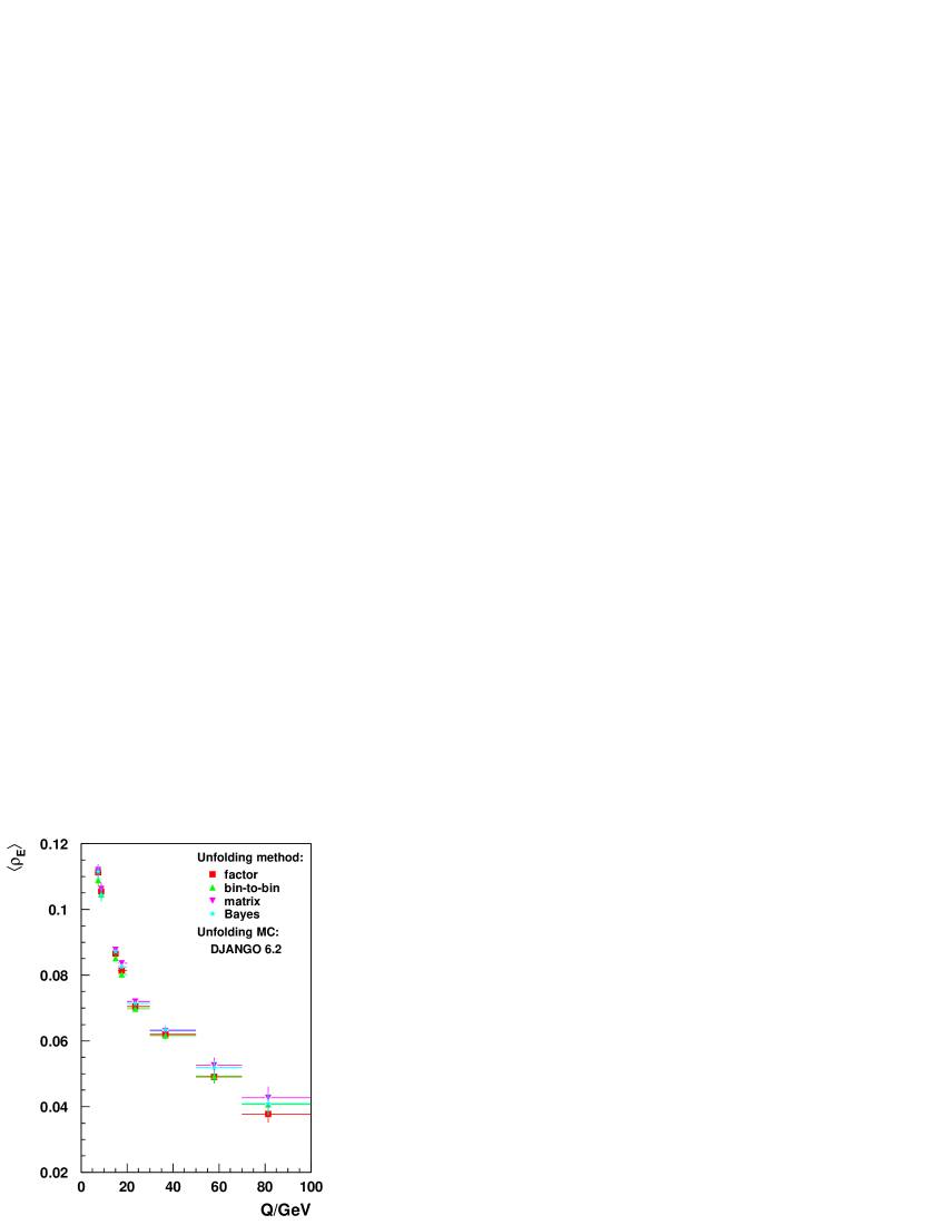
Abbildung 7.9: Unfolded means of $\tau_{P}$, $B_{P}$, $\rho_{E}$ and $\tau_{C}$ as a function of $Q$ for the four described correction schemes. DJANGO 6.2 served as unfolding MC. Note that the step from radiative to non-radiative hadron level can be accomplished by the factor or bin-to-bin methods only. The latter was employed for this purpose in case of the matrix and Bayes procedures. The error bars represent statistical uncertainties only.

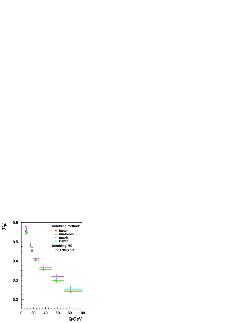
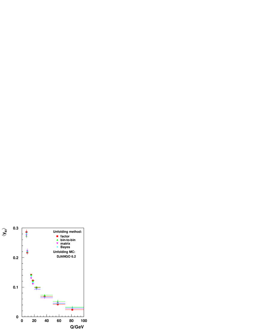
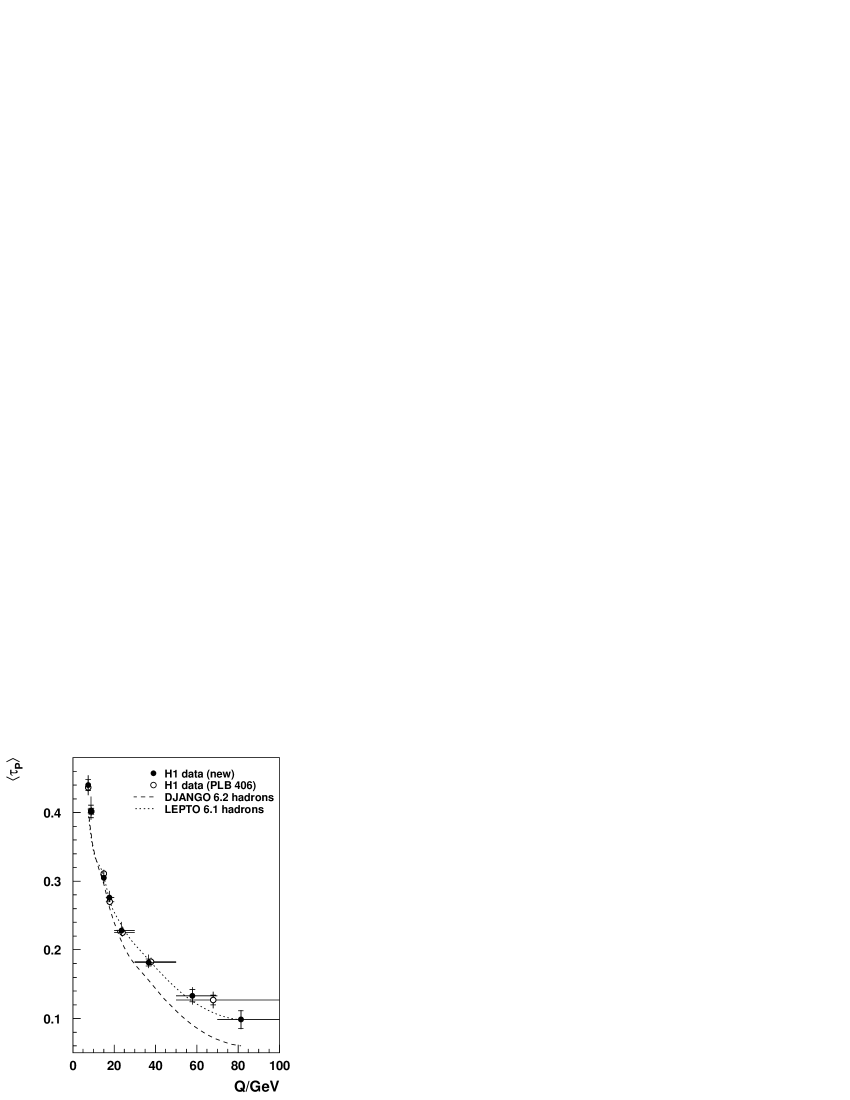
Abbildung 7.10: Unfolded means of $C_{P}$, $y_{fJ}$ and $y_{k_{t}}$ as a function of $Q$ for the four described correction schemes. DJANGO 6.2 served as unfolding MC. Note that the step from radiative to non-radiative hadron level can be accomplished by the factor or bin-to-bin methods only. The latter was employed for this purpose in case of the matrix and Bayes procedures. The error bars represent statistical uncertainties only.

Abbildung 7.11: Corrected means (full symbols) of $\tau_{P}$, $B_{P}$, $\rho_{E}$ and $\tau_{C}$ as a function of $Q$. The inner error bars represent the statistical uncertainty, the outer ones the total statistic and systematic uncertainty. They are compared with the hadron level mean values of the DJANGO 6.2 (dashed) and LEPTO 6.1 (dotted) MC and with already published results by H1 (hollow symbols).

Abbildung 7.12: Corrected means (full symbols) of $C_{P}$, $y_{fJ}$ and $y_{k_{t}}$ as a function of $Q$. The inner error bars represent the statistical uncertainty, the outer ones the total statistic and systematic uncertainty. They are compared with the hadron level mean values of the DJANGO 6.2 (dashed) and LEPTO 6.1 (dotted) MC.

Kapitel 8 NLO Integration Programs

According to the definition of the event shapes $F$ in section 4.2, they will take on non-trivial values, i.e. $F\neq 0$, when derived to ${\cal O}(\alpha_{s})$ at least. In terms of cross sections, the distributions $dn/dF$ may be written to LO accuracy as

$$\frac{1}{\sigma_{\rm tot}}\frac{d\sigma}{dF}=C_{1}(F)\alpha_{s}\,.$$ (8.1)

The first moment or mean value, characterizing the distribution in $F$ of an event sample in a simple way, now reads

$$\left<F\right>:=\frac{\int\limits_{0}^{F_{\rm max}}F\frac{d\sigma}{dF}dF}{\int\limits_{0}^{F_{\rm max}}\frac{d\sigma}{dF}dF}=\frac{1}{\sigma_{\rm tot}}\int\limits_{0}^{F_{\rm max}}F\frac{d\sigma}{dF}dF\,,$$ (8.2)

which can be expanded to LO in $\alpha_{s}$ as well:

$$\left<F\right>=c_{1,F}\alpha_{s}\,.$$ (8.3)

However, theoretical arguments show that the achieved precision of LO calculations is not sufficient to extract much information on pQCD from experimental data. Especially the concept of a running coupling constant $\alpha_{s}(\mu_{\scriptscriptstyle R})$, explained in the next section, requires the distributions and mean values to be known at least to NLO, i.e. ${\cal O}(\alpha_{s}^{2})$.

8.1 The Running Coupling Constant

Following an approach from [50], one may assume that a dimensionless quantity $\left<F\right>$ depends on a single energy scale $Q$ which is much larger than any other parameter measured in units of energy such that quark masses may be set to zero. Then, the conclusion is that $\left<F\right>$ has a constant value independent of $Q$; there is no other possibility to remove the dimension of $Q$. However, this is not true in a renormalizable quantum field theory such as QCD.

Perturbative calculations operating with “naked” charges $e_{0}$ (or masses $m_{0}$) of point particles have to deal with ultraviolet divergences occurring in the integrations of loop momenta $d^{4}k/(2\pi)^{4}$. The procedure allowing us to absorb these divergences in physical charges $e$ is called renormalization. Results concerning the (measured) physical charges are then all finite.

There exist several recipes how this can be done [51]. One of the most popular, also adopted in this analysis, is the modified minimal subtraction scheme $\overline{\rm MS}$, where the singularities are regulated by a reduction of the space-time dimensions to $n<4$:

$$\frac{d^{4}k}{(2\pi)^{4}}\rightarrow\mu^{2\epsilon}\frac{d^{4-2\epsilon}k}{(2\pi)^{4-2\epsilon}}\,.$$ (8.4)

At an arbitrary scale called renormalization scale $\mu_{\scriptscriptstyle R}$, the integrals are subdivided into finite and divergent parts for $\epsilon\rightarrow 0$. The singular terms (and some finite ones depending on the renormalization scheme) are then attributed to a renormalized charge $e$. However, the remaining finite terms also modify the charge $e$ or equivalently the coupling constant $\alpha:=e^{2}/4\pi$, which now explicitly varies with $\mu_{\scriptscriptstyle R}$!

Relating this to QCD, we have a strong coupling constant $\alpha_{s}:=g^{2}/4\pi$ containing $\mu_{\scriptscriptstyle R}$ — a second mass scale that enters the game. $\left<F\right>$ may therefore depend on the ratio $Q^{2}/\mu_{\scriptscriptstyle R}^{2}$. But since $\mu_{\scriptscriptstyle R}$ is an arbitrary parameter of the renormalization procedure, it should not make an appearance in physical observables like $\left<F\right>$. This can be expressed mathematically by

$$\mu_{\scriptscriptstyle R}^{2}\frac{d}{d\mu_{\scriptscriptstyle R}^{2}}\left<F\right>\left(Q^{2}/\mu_{\scriptscriptstyle R}^{2},\alpha_{s}\right)=\left[\mu_{\scriptscriptstyle R}^{2}\frac{\partial}{\partial\mu_{\scriptscriptstyle R}^{2}}+\mu_{\scriptscriptstyle R}^{2}\frac{\partial\alpha_{s}}{\partial\mu_{\scriptscriptstyle R}^{2}}\frac{\partial}{\partial\alpha_{s}}\right]\left<F\right>\left(Q^{2}/\mu_{\scriptscriptstyle R}^{2},\alpha_{s}\right)=0$$ (8.5)

or, using the notation

$$t = \ln\left(\frac{Q^{2}}{\mu_{\scriptscriptstyle R}^{2}}\right)\,,$$ (8.6)

$$\beta(\alpha_{s}) = \mu_{\scriptscriptstyle R}^{2}\frac{\partial\alpha_{s}}{\partial\mu_{\scriptscriptstyle R}^{2}}\,,$$ (8.7)

as

$$\left[-\frac{\partial}{\partial t}+\beta(\alpha_{s})\frac{\partial}{\partial\alpha_{s}}\right]\left<F\right>(e^{t},\alpha_{s})=0\,.$$ (8.8)

A solution to this partial differential equation can be given implicitly by defining the running coupling $\alpha_{s}(Q^{2})$ as

$$t=\int\limits_{\alpha_{s}}^{\alpha_{s}(Q^{2})}\frac{dx}{\beta(x)}\,,\quad\alpha_{s}:=\alpha_{s}(\mu_{\scriptscriptstyle R}^{2})$$ (8.9)

such that $\left<F\right>(1,\alpha_{s}(Q^{2}))$ fulfils eq. (8.8). The scale dependence of any $\left<F\right>$ calculated perturbatively now follows from $\alpha_{s}(Q^{2})$ provided eq. (8.9) could be solved. Since QCD is an asymptotically free theory, i.e. $\lim\limits_{Q\rightarrow\infty}\alpha_{s}(Q^{2})=0$, this can also be achieved by expanding the $\beta$-function of the Renormalization Group Equation (8.7) (RGE) in powers of $\alpha_{s}$:

$$\frac{\beta(\alpha_{s})}{4\pi}=-\sum\limits_{n=0}^{\infty}\beta_{n}\left(\frac{\alpha_{s}}{4\pi}\right)^{n+2}\,.$$ (8.10)

The first two coefficients defined that way are

$$\beta_{0} = \frac{33-2N_{f}}{3}\,,$$ (8.11)

$$\beta_{1} = \frac{306-38N_{f}}{3}\,,$$ (8.12)

where $N_{f}$ is the number of active flavours. $\beta_{2}$ and further coefficients are scheme dependent.

Retaining only the first term, the 1-loop solution for $\alpha_{s}(Q)$ can be written as

$$\alpha_{s}(Q)=\frac{\alpha_{s}(\mu_{\scriptscriptstyle R})}{1+\frac{\beta_{0}}{2\pi}\alpha_{s}(\mu_{\scriptscriptstyle R})\ln\left(\frac{Q}{\mu_{\scriptscriptstyle R}}\right)}\,.$$ (8.13)

Using this equation, $\alpha_{s}$ can be evaluated at any (sufficiently high) scale provided it is known at one point, say $M_{Z}$. Historically, a dimensional parameter $\Lambda$ derived from

$$\ln\frac{Q^{2}}{\Lambda^{2}}=-\int\limits_{\alpha_{s}(Q^{2})}^{\infty}\frac{dx}{\beta(x)}$$ (8.14)

was determined instead of $\alpha_{s}(M_{Z})$. The 1-loop formula then reads

$$\alpha_{s}(Q)=\frac{2\pi}{\beta_{0}\ln\left(\frac{Q}{\Lambda}\right)}$$ (8.15)

and demonstrates that $\Lambda$ indicates the scale at which the coupling would diverge if extrapolated outside the perturbative regime.

In principle, both approaches are equivalent and any measurement of $\alpha_{s}(M_{Z})$ can be converted into a corresponding value for $\Lambda$ and vice versa. The latter, however, has some disadvantages: It is not dimensionless, it depends on $N_{f}$ and on the renormalization scheme and — most important — there exist two slightly different definitions for $\Lambda$ in the literature [5, 50].

Except for the consistency check in section 9.2 employing $\Lambda_{5,\overline{\rm MS}}$, we therefore follow ref. [52] and apply the 2-loop equation according to

$$\alpha_{s}(Q)=\frac{\alpha_{s}(M_{Z})}{1+\alpha_{s}(M_{Z})\cdot L^{(n)}\left(\frac{Q}{M_{Z}}\right)}$$ (8.16)

where

$$L^{(1)}\left(\frac{Q}{M_{Z}}\right)=\frac{\beta_{0}}{2\pi}\ln\frac{Q}{M_{Z}}$$ (8.17)

reproduces the 1-loop formula above and

$$L^{(2)}\left(\frac{Q}{M_{Z}}\right)=\left(\frac{\beta_{0}}{2\pi}+\frac{\beta_{1}}{8\pi^{2}}\alpha_{s}(M_{Z})\right)\ln\frac{Q}{M_{Z}}$$ (8.18)

gives the 2-loop result.

Returning to $\left<F\right>$, the perturbative expression to all orders

$$\left<F\right>=\sum\limits_{n=1}^{\infty}c_{n}(\mu_{\scriptscriptstyle R})\alpha_{s}^{n}(\mu_{\scriptscriptstyle R})$$ (8.19)

does not depend on $\mu_{\scriptscriptstyle R}$. But we do not know all coefficients, and therefore any approximation by a truncated series does. To be more precise,

$$\mu_{\scriptscriptstyle R}^{2}\frac{d}{d\mu_{\scriptscriptstyle R}^{2}}\sum\limits_{n=1}^{N}c_{n}(\mu_{\scriptscriptstyle R})\alpha_{s}^{n}(\mu_{\scriptscriptstyle R})\propto{\cal O}(\alpha_{s}^{N+1}(\mu_{\scriptscriptstyle R}))\,.$$ (8.20)

According to current knowledge, the dependence on $\mu_{\scriptscriptstyle R}$ is much reduced if more terms are inserted. Hence, the theoretical uncertainty usually associated with the choice of scale, whose variation reflects the unknown higher orders, is diminished. Up to now, we merely considered $c_{1}$, which itself does not contain $\mu_{\scriptscriptstyle R}$, and the complete $\mu_{\scriptscriptstyle R}$-dependence stems from $\alpha_{s}(\mu_{\scriptscriptstyle R})$ and is rather large. It is reduced with the inclusion of $c_{2}(\mu_{\scriptscriptstyle R})\alpha_{s}^{2}(\mu_{\scriptscriptstyle R})$ with

$$c_{2}(Q)=c_{2}(1)+\frac{\beta_{0}}{2\pi}\ln\frac{\mu_{\scriptscriptstyle R}}{Q}c_{1}\,,$$ (8.21)

which can be calculated by the three NLO integration programs presented in the next sections.

8.2 NLO Integration Techniques

As mentioned in section 3.4 on the cross section to ${\cal O}(\alpha_{s})$, again infrared and collinear divergences are present in calculations to ${\cal O}(\alpha_{s}^{2})$ which cancel between real and virtual diagrams. Examples of real corrections to the QCDC and BGF processes with now three final state partons are given in fig. 8.1.

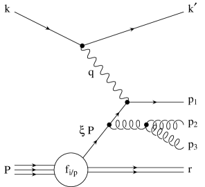
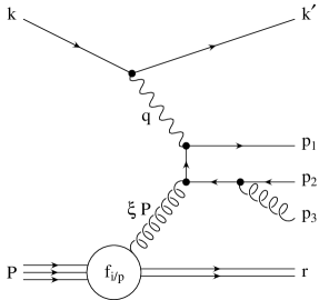
Abbildung 8.1: Examples of real corrections to QCDC (left) and BGF (right) Feynman graphs.

In order to eliminate the occurring singularities and obtain numerically stable results, the necessary cancellations were performed analytically for a certain jet algorithm in the programs DISJET [53] and PROJET [54]. However, these programs lack the flexibility to evaluate NLO corrections for arbitrary infrared-safe observables and they contain approximations that are inappropriate for certain phase space regions. Therefore, more elaborate methods have been developed that ensure the cancellations and evaluate numerical results for arbitrary observables. Basically, two such schemes are known: the phase space slicing method [55] and the subtraction method [28].

In the phase space slicing method, the separation of singular from non-singular phase space regions is done by surrounding partons with a small cone. Real emissions of partons outside the cone defined by $s_{ij}=(p_{i}+p_{j})^{2}>s_{\rm min}$, where $s_{\rm min}\approx 0.1\,{\rm GeV}^{2}$, are computed exactly. Inside the cone, soft and collinear approximations are used. A drawback of this procedure is the possibility of a residual dependence on the technical parameter $s_{\rm min}$. For any calculation it has to be established that a plateau has been reached for small enough cut-offs. In addition, this scheme prevents the integration of the event shape distributions $Fd\sigma/dF$ to be carried out over the whole phase space from zero to $F_{\rm max}$. Instead, a lower bound $F_{\rm cut}>0$ has to be imposed and $s_{\rm min}$ has to be adjusted accordingly. Moreover, the introduction of crossing functions [56], that have to be evaluated for every parton density parameterization, is required.

In case of the subtraction method, the singularities are cancelled point-by-point in phase space. A cut-off like $s_{\rm min}$ is not formally required by this scheme, although a tiny value of $s_{\rm min}\approx 10^{-8}$–$10^{-10}\,{\rm GeV}^{2}$ is applied to set the number of significant digits. Hence, the event shape distributions $Fd\sigma/dF$ can be integrated down to zero [57].

The first method is employed in the NLO integration program MEPJET [58], whereas the subtraction procedure is used in DISENT [59] and DISASTER++ [60]. All three programs, however, do not contain the full set of diagrams to ${\cal O}(\alpha_{s}^{2})$. Additional 2-loop virtual corrections from graphs like the ones in fig. 8.2 appear and are difficult to handle. Yet, they contribute as interference term to the Born process only and therefore do not affect the event shape distributions except for the bin at zero. The integral $\int_{0}^{F_{\rm max}}F\frac{d\sigma}{dF}dF$ still contains integrable divergences, but they are not harmful for DISENT or DISASTER++ [61]. A calculation of the total cross section $\int_{0}^{F_{\rm max}}\frac{d\sigma}{dF}dF$, needed for the normalization, to ${\cal O}(\alpha_{s}^{2})$ (i.e. NNLO), however, is not possible. A Taylor expansion of eq. (8.2)

$$\left<F\right> = \frac{\int\limits_{0}^{F_{\rm max}}F\frac{d\sigma}{dF}dF}{\int\limits_{0}^{F_{\rm max}}\frac{d\sigma}{dF}dF}$$ (8.22)

$$\approx \frac{a_{1}\alpha_{s}^{1}+a_{2}\alpha_{s}^{2}}{b_{0}\alpha_{s}^{0}+b_{1}\alpha_{s}^{1}+b_{2}\alpha_{s}^{2}}$$ (8.23)

$$= \frac{a_{1}}{b_{0}}\alpha_{s}^{1}+\frac{a_{2}-\frac{a_{1}b_{1}}{b_{0}}}{b_{0}}\alpha_{s}^{2}+{\cal O}(\alpha_{s}^{3})$$ (8.24)

shows that, owing to the property of $F$ to be zero in the QPM limit and hence $a_{0}=0$, $\sigma_{\rm tot}$ needs only be known to ${\cal O}(\alpha_{s})$ for $\left<F\right>$ to be still correct to ${\cal O}(\alpha_{s}^{2})$.

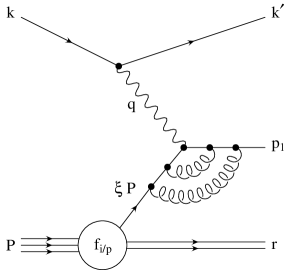
Abbildung 8.2: Examples of 2-loop virtual correction Feynman graphs.

8.3 First Comparisons of NLO Programs

In view of the complexity of the calculations and their implementations into program code, it is mandatory to compare the results where possible. A first comparison of MEPJET 1.4 and DISENT 0.0 was performed in [25]. Due to the phase space slicing method applied in MEPJET, the differential distributions for $F>F_{\rm cut}>0$ only could be considered. In order to keep $F_{\rm cut}$ small, a cut-off of $s_{\rm min}=0.01\,\,{\rm GeV}^{2}$ instead of $0.1\,\,{\rm GeV}^{2}$ was used. Nevertheless, the left-most bins extending down to zero should not be taken seriously, even if they accidentally do agree. Fig. 8.3 shows a perfect agreement of the LO spectra and, within the calculational precision of $3$–$5\%$, compatible results for the NLO distributions.

Abbildung 8.3: Differential distributions of $\tau_{P}$ for four out of seven investigated bins in $Q$. LO (left) and NLO (right) pQCD calculations of MEPJET 1.4 (hollow symbols) and DISENT 0.0 (full lines) are compared. The spectra for $\left<Q\right>=7.5$–$62.7\,{\rm GeV}$ are multiplied by factors of $10^{n}$, $n=0,1,2,3$.

With the advent of DISASTER++, a check of all three programs against each other was carried out and some discrepancies have been revealed [60]. Partially, these are understood and meanwhile an improved version DISENT 0.1 has been released. In event shape spectra like fig. 8.3, effects are hardly visible, but the mean values have increased considerably in the low $Q^{2}$ region compared to the calculations that entered in [23]. The worst case was the jet broadening $B_{P}$, whose mean value at $Q\approx 7.5\,{\rm GeV}$ rose by about $14\%$.

The most recent program versions are MEPJET 2.2, DISENT 0.1 and DISASTER++ 1.0.1. In this analysis only DISENT will be used, but more elaborate comparisons are under way in the DESY workshop on Monte Carlo Generators for HERA Physics.

Kapitel 9 DISENT Results

DISENT, the NLO integration program mainly employed here, is structured similarly to a MC event generator. A main routine generates configurations of parton momenta in the allowed phase space region — for our purposes defined by the cuts nos. • ‣ 5.5–• ‣ 5.5 of section 5.5 —, stores them in an event record and calculates the weight according to the matrix elements. Consequently, a user routine may analyze these events with respect to arbitrary infrared and collinear safe observables. For physical cross sections, the weights have to be multiplied by the strong coupling constant raised to the proper power and by weights extracted from the pdfs of the proton. These are not inherent to DISENT but must be gathered from somewhere else, e.g. the PDFLIB [39]. As standard options we use the set MRSA’-115 [62] and $N_{f}=5$ as number of active flavours. Note that DISENT currently neglects quark masses as well as electroweak corrections proportional to $Q^{2}/(Q^{2}+M_{Z}^{2})$ and $(Q^{2}/(Q^{2}+M_{Z}^{2}))^{2}$. Fortunately, only the highest $Q$-bin investigated with $\left<Q\right>=81.32\,{\rm GeV}$ may be affected noticeably [13]. In the near future, DISENT may be extended to include the electroweak terms [63].

In distinction to MC generators, however, several different but correlated event records, in total $14$, are produced for one DISENT “event.”  They correspond to contributions of real and virtual diagrams plus counter terms that ensure the necessary cancellation of divergences. These contributions have coupled weights that are positive as well as negative. For the error evaluation, it is mandatory that these weights are allowed to counterbalance each other before finally e.g. being histogrammed. This may be done by creating an intermediate array or histogram, where only the contributions of one event are entered. All bins not empty at the end are then transferred to the final array with their respective weights. A more detailed program description can be found in [64].

9.1 Evaluation of the Statistical Uncertainty

Given the framework of the DISENT program, the calculation of differential distributions $d\sigma/dF$ and mean values $\left<F\right>$ is straightforward. Positive and negative weights of the different contributions are summed up. Yet, the evaluation of the statistical uncertainties, where the technique of intermediate histograms is presupposed, is more involved.

First, we want to consider cross sections that can be written as a sum of weights $w_{i}$, given by DISENT, which are already normalized to the number of events $N$:

$$\sigma=\sum\limits_{i=1}^{N}w_{i}\,.$$ (9.1)

By reintroducing unnormalized weights $v_{i}$, one obtains

$$\sigma=\frac{1}{N}\sum\limits_{i=1}^{N}v_{i}=\left<v\right>\,,$$ (9.2)

demonstrating that $\sigma$ is computed analogously to a mean value. Its statistical uncertainty can be estimated by

$$\Delta\sigma = \sqrt{\frac{1}{N-1}\left(\left<v^{2}\right>-\left<v\right>^{2}\right)}$$

$$= \sqrt{\frac{1}{N-1}\left(\frac{1}{N}\sum\limits_{i=1}^{N}v_{i}^{2}-\frac{1}{N^{2}}\left(\sum\limits_{i=1}^{N}v_{i}\right)^{2}\,\right)}$$

$$= \sqrt{\frac{1}{N-1}\left(N\sum\limits_{i=1}^{N}w_{i}^{2}-\left(\sum\limits_{i=1}^{N}w_{i}\right)^{2}\,\right)}\,.$$

With $N\approx N-1$, this finally gives

$$\Delta\sigma=\sqrt{\sum\limits_{i=1}^{N}w_{i}^{2}-\frac{\left(\sum\limits_{i=1}^{N}w_{i}\right)^{2}}{N}}\,,$$ (9.4)

which in the limit of very large $N$ becomes

$$\Delta\sigma=\sqrt{\sum\limits_{i=1}^{N}w_{i}^{2}}\,.$$ (9.5)

For our purposes the second term is not negligible and formula (9.4) has to be applied. Turning to the event shape means

$$\left<F\right>=\frac{\sum\limits_{i=1}^{N}F_{i}w_{i}}{\sum\limits_{i=1}^{N}w_{i}^{{}^{\prime}}}$$ (9.6)

one could be misled to the assumption that a similar uncertainty as in eq. (9.1) could be derived here. Yet, formula (9.6) emphasizes that the weights $w_{i}$ and $w_{i}^{{}^{\prime}}$ are not identical because the numerator is evaluated to ${\cal O}(\alpha_{s}^{2})$ and the cross section in the denominator to ${\cal O}(\alpha_{s})$ only. Instead, the uncertainties have to be estimated separately, and afterwards the error of the quotient can be obtained by the usual formulae. The final result reads:

$$\Delta\left<F\right>=\left<F\right>\sqrt{\frac{\sum\limits_{i=1}^{N}\left(F_{i}w_{i}\right)^{2}}{\left(\sum\limits_{i=1}^{N}F_{i}w_{i}\right)^{2}}+\frac{\sum\limits_{i=1}^{N}w_{i}^{{}^{\prime}2}}{\left(\sum\limits_{i=1}^{N}w_{i}^{{}^{\prime}}\right)^{2}}-\frac{2}{N}}\,.$$ (9.7)

As a cross-check, the same DISENT 0.0 calculation has been repeated about a hundred times with different seeds of the random number generator for $0.1$, $0.2$, $0.5$ and $1.0$ million generated parton events each. Fig. 9.1 shows on the left-hand side histograms of the obtained cross sections $\sigma_{\rm tot}$ and mean values $\left<\tau_{P}\right>$ together with the fit of a Gaussian distribution for half a million events. It describes the distribution of the results well and its standard deviation is compatible with the deduced uncertainty ${\rm RMS}_{\rm calc}$. The right-hand side presents the dependence of the uncertainties for both, the statistical and the computational derivation, on the number of events produced. It nicely exhibits errors shrinking proportional to $1/\sqrt{N}$. The computation underestimates only slightly the statistically achieved variance.

The error bars in differential distributions are evaluated according to eq. (9.5).

Abbildung 9.1: Left: Histograms of $\sigma_{\rm tot}$ (top) and $\left<\tau_{P}\right>$ (bottom) plus Gaussian fit resulting from $117$ DISENT 0.0 calculations with half a million events each. ${\rm RMS}_{\rm calc}$ denotes the on average estimated standard deviation. Right: Dependence on $1/\sqrt{N}$ of the statistical (full symbols) and computational (hollow symbols) uncertainty estimates for $\sigma_{\rm tot}$ and $\left<\tau_{P}\right>$.

9.2 $\char 120\relax$ -Dependence

$\alpha_{s}(M_{Z})$ is the fundamental parameter of QCD that has to be determined by experiment. An assumption on it, however, is already contained in our cross section and mean value calculations. Therefore, they cannot directly be used to extract information from our data. In [25] and [23] this problem was avoided by fitting eq. (8.19) up to ${\cal O}(\alpha_{s}^{2})$ to the obtained mean values of each event shape. The resulting coefficients $c_{1,F}$ and $c_{2,F}$ are subsequently employed for an $\alpha_{s}(M_{Z})$-dependent parameterization of the event shape means.

In contrast to $e^{+}e^{-}$ physics, where $c_{1,F}$ and $c_{2,F}$ truly are pure numbers (s. e.g. [65]), this is not the case in $ep$ DIS because in addition to the matrix elements $x$-dependent pdfs enter their evaluation. In general, the coefficients will therefore be functions of $x$ which was taken into account in an approximate way only by the above ansatz. Fig. 9.2 presents as examples for a strong — the “worst” case being $y_{k_{t}}$ — and a weak variation of the mean values with $x$ curves of $\left<\tau_{P}\right>$ and $\left<C_{P}\right>$ versus $Q$ for four different bins in $x$. Note that in this investigation the two highest $Q$-bins were merged.

Abbildung 9.2: Mean values of $\tau_{P}$ (left) and $C_{P}$ (right) versus $Q$ in four different bins of $x$.

A solution to this problem is the direct calculation of $c_{1,F}$ and $c_{2,F}$ for every $Q$-bin with its specific $x$-range separately. This method corresponds to an approximation of functions $c_{n,F}(x)$ by step functions instead of one suitably chosen number.

As a consistency check, the perturbative mean values at LO and NLO are fit with the coefficients derived in the same computation. The outcome for $\Lambda_{5,\overline{\rm MS}}$ should be identical to the initial choice, that is $\Lambda_{5,\overline{\rm MS}}=179\,\,{\rm MeV}$ for MRSA’-115. The achieved fits for $\left<\tau_{P}\right>$ and $\left<C_{P}\right>$ are displayed in fig. 9.3. Again, the much steeper steps for $\left<\tau_{P}\right>$ indicate its stronger $x$-dependence. The $\Lambda_{5,\overline{\rm MS}}$ values extracted turn out to be very well compatible with the expectation for all event shapes except for the jet broadening $B_{P}$ in NLO! This may be a hint that there is a problem in the DISENT 0.1 calculations at low $Q^{2}$.

Abbildung 9.3: Fits (dashed and full lines) of $\Lambda_{5,\overline{\rm MS}}$ for the LO (hollow symbols) and NLO (full symbols) means of $\tau_{P}$ (left) and $C_{P}$ (right). The steps express the $x$-dependence of the perturbative coefficients $c_{1,F}$ and $c_{2,F}$.

9.3 Final Perturbative Coefficients

The final results obtained with DISENT 0.1 are compiled in the tables 9.1–9.8. The first one contains the mean $Q$- and $x$-values to NLO for the eight bins of section 5.5 as well as the LO and NLO cross sections. The latter are differentiated by indices “1H” and “2H” to indicate whether the CH alone (1H, energy cut no. • ‣ 5.5) or both hemispheres (2H, no energy cut) are allowed to contribute to the hadronic final state. To LO there is no difference because the only parton available has $E^{\star}=Q/2$ and runs into the CH by definition.

Tables 9.2–9.8 comprise the mean values of all event shapes for our standard pdf set MRSA’-115 and the perturbative coefficients $c_{1,F}$ and $c_{2,F}$ needed for the $\alpha_{s}(M_{Z})$-dependent parameterization of the means.

$\left<Q\right>/\,{\rm GeV}$	$\left<x\right>$	$\sigma_{\rm LO}/pb$	$\sigma_{\rm NLO,1H}/pb$	$\sigma_{\rm NLO,2H}/pb$
$7.46$	$4.58\cdot 10^{-3}$	$2519.9\pm 0.3$	$2232.5\pm 0.4$	$2402.6\pm 0.4$
$8.80$	$7.21\cdot 10^{-3}$	$2357.5\pm 0.4$	$2111.9\pm 0.5$	$2245.8\pm 0.5$
$14.95$	$1.60\cdot 10^{-2}$	$534.4\pm 0.1$	$484.4\pm 0.1$	$503.8\pm 0.1$
$17.73$	$2.16\cdot 10^{-2}$	$584.7\pm 0.1$	$533.4\pm 0.1$	$551.1\pm 0.1$
$23.75$	$3.16\cdot 10^{-2}$	$465.8\pm 0.1$	$428.4\pm 0.1$	$438.9\pm 0.1$
$36.69$	$5.80\cdot 10^{-2}$	$156.2\pm 0.1$	$145.9\pm 0.1$	$147.9\pm 0.1$
$57.61$	$1.09\cdot 10^{-1}$	$24.79\pm 0.02$	$23.63\pm 0.02$	$23.75\pm 0.02$
$80.76$	$1.74\cdot 10^{-1}$	$7.502\pm 0.006$	$7.291\pm 0.006$	$7.305\pm 0.006$

Tabelle 9.1: Mean $Q$- and $x$-values as well as the LO and NLO cross sections as calculated by DISENT 0.1. The indices “1H” and “2H” differentiate between cross sections with and without the minimal energy cut in the CH.

$\left<Q\right>/\,{\rm GeV}$	$\left<\tau_{P}\right>_{\rm LO}$	$\left<\tau_{P}\right>_{\rm NLO}$	$c_{1,\tau_{P}}$	$c_{2,\tau_{P}}$
$7.46$	$0.2633\pm 0.0001$	$0.3377\pm 0.0014$	$1.4559\pm 0.0006$	$2.250\pm 0.041$
$8.80$	$0.2391\pm 0.0001$	$0.3070\pm 0.0012$	$1.3735\pm 0.0008$	$2.226\pm 0.038$
$14.95$	$0.1847\pm 0.0001$	$0.2387\pm 0.0009$	$1.1895\pm 0.0008$	$2.222\pm 0.038$
$17.73$	$0.1684\pm 0.0001$	$0.2173\pm 0.0008$	$1.1217\pm 0.0007$	$2.159\pm 0.037$
$23.75$	$0.1453\pm 0.0002$	$0.1871\pm 0.0013$	$1.0209\pm 0.0011$	$2.065\pm 0.062$
$36.69$	$0.1138\pm 0.0001$	$0.1480\pm 0.0007$	$0.8622\pm 0.0011$	$1.978\pm 0.041$
$57.61$	$0.0846\pm 0.0002$	$0.1113\pm 0.0008$	$0.6909\pm 0.0014$	$1.811\pm 0.055$
$80.76$	$0.0654\pm 0.0002$	$0.0864\pm 0.0006$	$0.5622\pm 0.0022$	$1.604\pm 0.043$

Tabelle 9.2: Mean values and perturbative coefficients for $\tau_{P}$ as derived from DISENT 0.1.

$\left<Q\right>/\,{\rm GeV}$	$\left<B_{P}\right>_{\rm LO}$	$\left<B_{P}\right>_{\rm NLO}$	$c_{1,B_{P}}$	$c_{2,B_{P}}$
$7.46$	$0.3923\pm 0.0001$	$0.2524\pm 0.0018$	$2.1696\pm 0.0007$	$-3.444\pm 0.049$
$8.80$	$0.3604\pm 0.0002$	$0.2510\pm 0.0018$	$2.0699\pm 0.0009$	$-2.894\pm 0.052$
$14.95$	$0.2879\pm 0.0001$	$0.2309\pm 0.0014$	$1.8545\pm 0.0009$	$-1.847\pm 0.051$
$17.73$	$0.2659\pm 0.0001$	$0.2215\pm 0.0012$	$1.7713\pm 0.0008$	$-1.513\pm 0.047$
$23.75$	$0.2350\pm 0.0002$	$0.2063\pm 0.0013$	$1.6515\pm 0.0013$	$-1.034\pm 0.056$
$36.69$	$0.1921\pm 0.0002$	$0.1795\pm 0.0009$	$1.4565\pm 0.0015$	$-0.437\pm 0.047$
$57.61$	$0.1521\pm 0.0002$	$0.1528\pm 0.0007$	$1.2431\pm 0.0021$	$0.245\pm 0.042$
$80.76$	$0.1254\pm 0.0002$	$0.1309\pm 0.0005$	$1.0798\pm 0.0023$	$0.571\pm 0.034$

Tabelle 9.3: Mean values and perturbative coefficients for $B_{P}$ as derived from DISENT 0.1.

$\left<Q\right>/\,{\rm GeV}$	$\left<\rho_{E}\right>_{\rm LO}$	$\left<\rho_{E}\right>_{\rm NLO}$	$c_{1,\rho_{E}}$	$c_{2,\rho_{E}}$
$7.46$	$0.0464\pm 0.0001$	$0.0538\pm 0.0006$	$0.2564\pm 0.0002$	$0.243\pm 0.017$
$8.80$	$0.0437\pm 0.0001$	$0.0522\pm 0.0005$	$0.2509\pm 0.0002$	$0.293\pm 0.014$
$14.95$	$0.0367\pm 0.0001$	$0.0464\pm 0.0004$	$0.2363\pm 0.0002$	$0.405\pm 0.015$
$17.73$	$0.0347\pm 0.0001$	$0.0445\pm 0.0003$	$0.2309\pm 0.0003$	$0.434\pm 0.014$
$23.75$	$0.0316\pm 0.0001$	$0.0406\pm 0.0009$	$0.2222\pm 0.0004$	$0.448\pm 0.040$
$36.69$	$0.0274\pm 0.0001$	$0.0367\pm 0.0003$	$0.2076\pm 0.0004$	$0.537\pm 0.019$
$57.61$	$0.0233\pm 0.0001$	$0.0321\pm 0.0004$	$0.1907\pm 0.0007$	$0.589\pm 0.028$
$80.76$	$0.0204\pm 0.0001$	$0.0279\pm 0.0002$	$0.1761\pm 0.0009$	$0.569\pm 0.017$

Tabelle 9.4: Mean values and perturbative coefficients for $\rho_{E}$ as derived from DISENT 0.1.

$\left<Q\right>/\,{\rm GeV}$	$\left<\tau_{C}\right>_{\rm LO}$	$\left<\tau_{C}\right>_{\rm NLO}$	$c_{1,\tau_{C}}$	$c_{2,\tau_{C}}$
$7.46$	$0.0701\pm 0.0001$	$0.0907\pm 0.0010$	$0.3876\pm 0.0003$	$0.620\pm 0.028$
$8.80$	$0.0664\pm 0.0001$	$0.0872\pm 0.0008$	$0.3816\pm 0.0004$	$0.675\pm 0.025$
$14.95$	$0.0569\pm 0.0001$	$0.0770\pm 0.0007$	$0.3666\pm 0.0004$	$0.814\pm 0.026$
$17.73$	$0.0542\pm 0.0001$	$0.0738\pm 0.0006$	$0.3607\pm 0.0004$	$0.854\pm 0.025$
$23.75$	$0.0500\pm 0.0001$	$0.0688\pm 0.0006$	$0.3515\pm 0.0006$	$0.911\pm 0.030$
$36.69$	$0.0443\pm 0.0001$	$0.0618\pm 0.0005$	$0.3357\pm 0.0006$	$0.999\pm 0.030$
$57.61$	$0.0389\pm 0.0001$	$0.0550\pm 0.0005$	$0.3179\pm 0.0007$	$1.077\pm 0.034$
$80.76$	$0.0348\pm 0.0001$	$0.0490\pm 0.0004$	$0.2991\pm 0.0009$	$1.073\pm 0.028$

Tabelle 9.5: Mean values and perturbative coefficients for $\tau_{C}$ as derived from DISENT 0.1.

$\left<Q\right>/\,{\rm GeV}$	$\left<C_{P}\right>_{\rm LO}$	$\left<C_{P}\right>_{\rm NLO}$	$c_{1,C_{P}}$	$c_{2,C_{P}}$
$7.46$	$0.2708\pm 0.0002$	$0.3470\pm 0.0035$	$1.4977\pm 0.0010$	$2.304\pm 0.096$
$8.80$	$0.2570\pm 0.0002$	$0.3325\pm 0.0031$	$1.4765\pm 0.0013$	$2.472\pm 0.091$
$14.95$	$0.2207\pm 0.0002$	$0.2945\pm 0.0024$	$1.4220\pm 0.0015$	$3.000\pm 0.094$
$17.73$	$0.2103\pm 0.0002$	$0.2826\pm 0.0021$	$1.4008\pm 0.0015$	$3.151\pm 0.088$
$23.75$	$0.1945\pm 0.0003$	$0.2638\pm 0.0024$	$1.3679\pm 0.0022$	$3.371\pm 0.112$
$36.69$	$0.1728\pm 0.0003$	$0.2374\pm 0.0019$	$1.3109\pm 0.0024$	$3.689\pm 0.107$
$57.61$	$0.1522\pm 0.0004$	$0.2126\pm 0.0019$	$1.2451\pm 0.0033$	$4.049\pm 0.124$
$80.76$	$0.1371\pm 0.0004$	$0.1909\pm 0.0013$	$1.1796\pm 0.0044$	$4.063\pm 0.095$

Tabelle 9.6: Mean values and perturbative coefficients for $C_{P}$ as derived from DISENT 0.1.

$\left<Q\right>/\,{\rm GeV}$	$\left<y_{fJ}\right>_{\rm LO}$	$\left<y_{fJ}\right>_{\rm NLO}$	$c_{1,y_{fJ}}$	$c_{2,y_{fJ}}$
$7.46$	$0.1694\pm 0.0001$	$0.1575\pm 0.0007$	$0.9369\pm 0.0004$	$-0.197\pm 0.020$
$8.80$	$0.1553\pm 0.0001$	$0.1493\pm 0.0007$	$0.8918\pm 0.0005$	$-0.043\pm 0.021$
$14.95$	$0.1219\pm 0.0001$	$0.1253\pm 0.0006$	$0.7852\pm 0.0005$	$0.259\pm 0.021$
$17.73$	$0.1119\pm 0.0001$	$0.1172\pm 0.0005$	$0.7452\pm 0.0005$	$0.341\pm 0.020$
$23.75$	$0.0976\pm 0.0001$	$0.1054\pm 0.0005$	$0.6859\pm 0.0007$	$0.473\pm 0.024$
$36.69$	$0.0779\pm 0.0001$	$0.0875\pm 0.0004$	$0.5905\pm 0.0007$	$0.618\pm 0.019$
$57.61$	$0.0594\pm 0.0001$	$0.0697\pm 0.0003$	$0.4854\pm 0.0007$	$0.739\pm 0.018$
$80.76$	$0.0470\pm 0.0001$	$0.0564\pm 0.0002$	$0.4052\pm 0.0009$	$0.739\pm 0.014$

Tabelle 9.7: Mean values and perturbative coefficients for $y_{fJ}$ as derived from DISENT 0.1.

$\left<Q\right>/\,{\rm GeV}$	$\left<y_{k_{t}}\right>_{\rm LO}$	$\left<y_{k_{t}}\right>_{\rm NLO}$	$c_{1,y_{k_{t}}}$	$c_{2,y_{k_{t}}}$
$7.46$	$0.2138\pm 0.0001$	$0.2942\pm 0.0004$	$1.1825\pm 0.0004$	$2.529\pm 0.016$
$8.80$	$0.1803\pm 0.0001$	$0.2366\pm 0.0003$	$1.0348\pm 0.0005$	$1.929\pm 0.016$
$14.95$	$0.1214\pm 0.0001$	$0.1514\pm 0.0002$	$0.7818\pm 0.0004$	$1.299\pm 0.013$
$17.73$	$0.1045\pm 0.0001$	$0.1288\pm 0.0002$	$0.6960\pm 0.0004$	$1.123\pm 0.011$
$23.75$	$0.0830\pm 0.0001$	$0.1008\pm 0.0002$	$0.5830\pm 0.0005$	$0.920\pm 0.013$
$36.69$	$0.0562\pm 0.0001$	$0.0676\pm 0.0001$	$0.4256\pm 0.0004$	$0.686\pm 0.009$
$57.61$	$0.0349\pm 0.0001$	$0.0423\pm 0.0001$	$0.2851\pm 0.0007$	$0.515\pm 0.008$
$80.76$	$0.0235\pm 0.0001$	$0.0287\pm 0.0001$	$0.2015\pm 0.0009$	$0.405\pm 0.005$

Tabelle 9.8: Mean values and perturbative coefficients for $y_{k_{t}}$ as derived from DISENT 0.1.

Kapitel 10 Power Corrections

To get a first impression of the extent to which pQCD is able to approximate the data, figs. 10.1 and 10.2 present the normalized differential distributions of the seven investigated event shapes, corrected to hadron level, in comparison with DISENT 0.1 NLO calculations. Note that the first data bin was left out in both normalizations. This is necessary since according to section 8.2 it is not possible to go down to $F=0$ in ${\cal O}(\alpha_{s}^{2})$. Starting with bin one, the NLO histogram could alternatively be normalized to $\sigma_{\rm NLO}$ yielding a slight mismatch by a factor of $\sigma_{\rm NLO}/\sigma_{\rm NNLO}$. Except for a small shift in height complicating a comparison of shapes, the conclusions would not change.

Obviously, there are large discrepancies between data and the NLO predictions. Common to all event shapes, however, is the clear tendency that the description of data improves considerably with rising $Q$; to what degree depends on the variable under consideration. $y_{fJ}$ and $y_{k_{t}}$ exhibit a very fast convergence hinting at small hadronization corrections, whereas the prediction for $C_{P}$ approaches the data slowly.

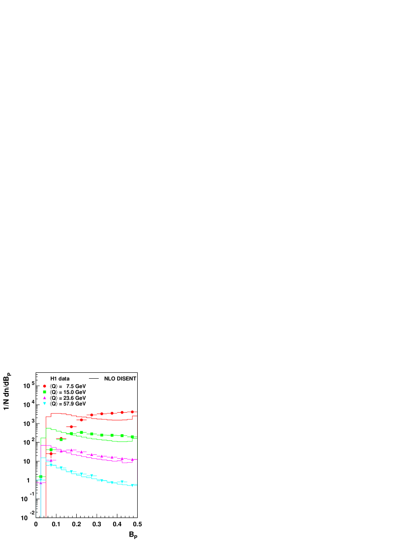
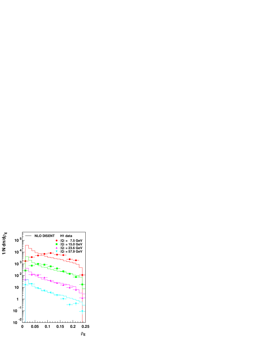
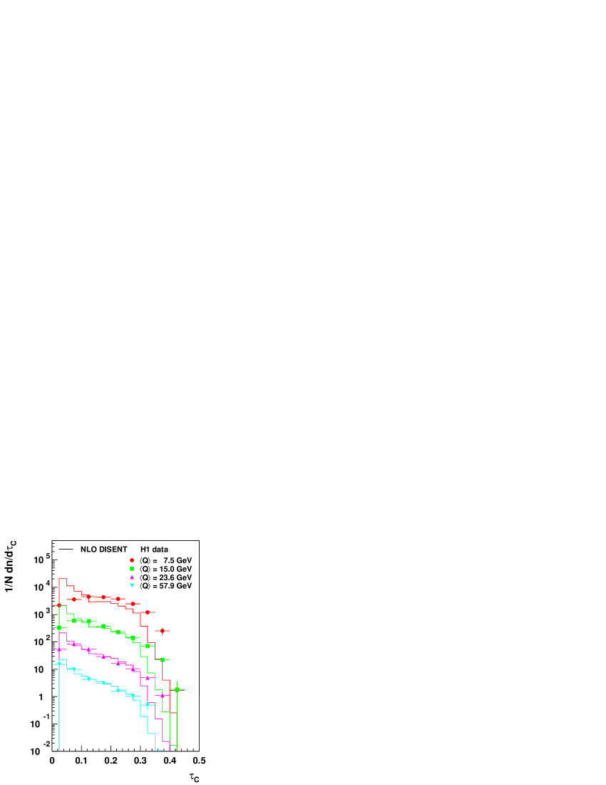
Abbildung 10.1: Normalized differential distributions of the event shapes $\tau_{P}$, $B_{P}$, $\rho_{E}$ and $\tau_{C}$ corrected to hadron level. H1 data (full symbols) are compared with DISENT 0.1 NLO calculations (full lines) for four out of eight investigated bins in $Q$. The spectra for $\left<Q\right>=7.5$–$57.9\,{\rm GeV}$ are multiplied by factors of $10^{n}$, $n=0,1,2,3$. The error bars represent statistical uncertainties only. Note that the first data bin was left out in both normalizations.

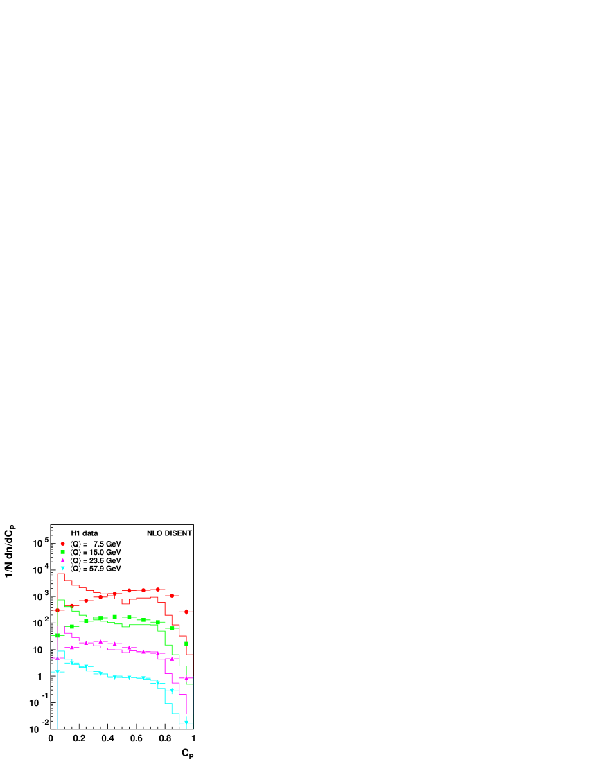
Abbildung 10.2: Normalized differential distributions of the event shapes $C_{P}$, $y_{fJ}$ and $y_{k_{t}}$ corrected to hadron level. H1 data (full symbols) are compared with DISENT 0.1 NLO calculations (full lines) for four out of eight investigated bins in $Q$. The spectra for $\left<Q\right>=7.5$–$57.9\,{\rm GeV}$ are multiplied by factors of $10^{n}$, $n=0,1,2,3$. The error bars represent statistical uncertainties only. Note that the first data bin was left out in both normalizations.

Turning back to the mean values $\left<F\right>$, we can, except for the $y$ shapes, expect them to be substantially larger than predicted by pQCD with decreasing differences for increasing $Q$. Indeed, physical quantities receive, in addition to pQCD, non-perturbative contributions which basically behave power-like, i.e. $\propto 1/Q^{p}$, hence called power corrections. The cross section $\mbox{$e^{+}e^{-}$\leavevmode\nobreak\ }\rightarrow{\rm hadrons}$, $\sigma_{\rm had}$, for example exhibits a $1/Q^{4}$-term which is also understandable on theoretical grounds [66]. Less inclusive variables like event shapes are not as well-behaved as $\sigma_{\rm had}$ and reveal $1/Q$-corrections that are sizable even at $Q=M_{Z}$ [67]. They can be made plausible in the framework of a longitudinal phase space or tube model [68], which essentially is the simplest version of the string fragmentation implemented in JETSET. One possibility to compare with pQCD is based on hadronization models like the one implemented in JETSET by unfolding the data in a third correction step to some kind of (ambiguous) parton level.

We do not follow this recipe. Instead, we will call upon explicit formulae trying to parameterize these effects. They are presented in sections 10.1 and 10.3 for the tube model and a new approach respectively. The main goal of this work is to test these models.

10.1 The Tube Model

Measurements of the momentum spectra of secondary particles produced by a primary parton of energy $E_{0}=Q/2$ approximately obey rather simple scaling laws [3]. Characterizing a particular secondary by $E$, $p_{t}$, $p_{l}$ and $m$ with respect to the direction of the original parton, the distribution in $p_{t}$, $\rho(p_{t})$, decreases exponentially almost independently of $E_{0}$ and $p_{l}$, whereas the distribution in $p_{l}$ rises proportional to $E_{0}$. Making use of the rapidity variable $y_{R}$ (s. eq. (5.3)),

$$y_{R}:=\frac{1}{2}\ln\frac{E+p_{l}}{E-p_{l}}=\ln\frac{E+p_{l}}{\sqrt{p_{t}^{2}+m^{2}}}\,,$$ (10.1)

with the property $dy_{R}=dp_{l}/E$, this can be expressed in the form of

$$\Phi(y_{R},p_{t})=B\cdot\rho(p_{t})\,.$$ (10.2)

$B$ is the (constant) number of hadrons per unity in rapidity and $\Phi$ the distribution function of light hadrons in the produced jet corresponding to a tube in $(y_{R},p_{t})$-space. Following refs. [50, 69], the energy $E_{j}$ and longitudinal momentum $P_{l,j}$ of a jet of length $y_{R,{\rm max}}$ in rapidity can be estimated by:

$$E_{j}= \int\limits_{0}^{y_{R,{\rm max}}}\int\limits_{0}^{\infty}E\cdot B\rho(p_{t})dp_{t}dy_{R} \approx\lambda\sinh y_{R,{\rm max}}\approx p_{l,{\rm max}}\approx E_{0}\,,$$ (10.3)

$$P_{l,j}= \int\limits_{0}^{y_{R,{\rm max}}}\int\limits_{0}^{\infty}p_{l,j}\cdot B\rho(p_{t})dp_{t}dy_{R} \approx\lambda(\cosh y_{R,{\rm max}}-1)\approx E_{0}-\lambda\,.$$ (10.4)

Recall that $E=m_{t}\cosh y_{R}$ and $p_{l}=m_{t}\sinh y_{R}$ with the transverse mass

$$m_{t}:=\sqrt{p_{t}^{2}+m^{2}}\approx p_{t}$$ (10.5)

for light hadrons. $\lambda$ is proportional to the average transverse momentum:

$$\lambda:=B\int\limits_{0}^{\infty}p_{t}\rho(p_{t})dp_{t}\,.$$ (10.6)

The power corrections to mean $\tau=1-$thrust and jet mass now become

$$\left<\tau\right>^{\rm pow} =1-\frac{P_{l,j}}{E_{j}}\approx 1-\frac{E_{0}-\lambda}{E_{0}}= \frac{2\lambda}{Q}\,,$$ (10.7)

$$\left<\rho\right>^{\rm pow} \approx\frac{E_{j}^{2}-P_{l,j}^{2}}{Q^{2}}\approx\frac{E_{0}^{2}-(E_{0}-\lambda)^{2}}{Q^{2}}\approx \frac{\lambda}{Q}\,.$$ (10.8)

With $B\approx 2$ and $\left<p_{t}\right>\approx 0.3\,{\rm GeV}$ [69], we can estimate $\lambda\approx 0.6\,{\rm GeV}$. Testing this simple ansatz with event shapes in $ep$ DIS is the topic of the next section.

10.2 $1/Q^{\char 112\relax}$ -Fits

The input for all fits performed here and in section 10.4 consists of the corrected data means of table 7.1 and the perturbative coefficients given in tables 9.2–9.8 together with their statistical uncertainties. Systematic uncertainties are not taken into account; they will be analyzed in section 10.5.

The standard fit procedure employs the method of least squares (s. e.g. [70]) to determine the best estimates for the parameters of the supplied model. Technically, this is accomplished by using the program MINUIT [71] which additionally provides the $\chi^{2}$-value and, where appropriate, the maximally encountered correlation $\kappa$. In the tables collecting the results, the reduced $\chi^{2}$-values, i.e. $\chi^{2}$ divided by the number of degrees of freedom (dof), are entered. For one- and two-parameter fits we have seven respectively six dofs yielding a maximal $\chi^{2}/{\rm dof}\approx 2$ at a confidence level of $5\%$.

The first test carried out is to allow a variation of $\alpha_{s}(M_{Z})$ in the perturbative expression

$$\left<F\right>^{\rm pert}=c_{1,F}(x)\,\alpha_{s}(\mu_{\scriptscriptstyle R})+\left(c_{2,F}(x)+\frac{\beta_{0}}{2\pi}\ln\frac{\mu_{\scriptscriptstyle R}}{Q}c_{1,F}(x)\right)\alpha_{s}^{2}(\mu_{\scriptscriptstyle R})$$ (10.9)

only, where, for the time being, $\mu_{\scriptscriptstyle R}$ is identified with $Q$. As can be seen from table 10.1, this works surprisingly well except for $B_{P}$. Seemingly, the decrease of $\left<F\right>$ with $Q$ can be accounted for by the logarithmic $Q$-dependence of $\alpha_{s}$ as long as $\alpha_{s}(M_{Z})$ may be adapted to the corresponding hadronization correction. Compared to the world average $\alpha_{s}(M_{Z})=0.119$ [5], we obtain high results for $\tau_{P}$ and $B_{P}$, very high ones for $\rho_{E}$, $\tau_{C}$, $C_{P}$ and lower values for $y_{fJ}$, $y_{k_{t}}$. Taking this as an indication for the impact of hadronization, it can be concluded that our event shapes are affected by medium, large and small (negative) corrections respectively.

Sometimes, the ratio of NLO to LO results, the $K$-factor, is considered to signal big effects of higher orders. However, although evaluating them for $\tau_{P}$ and $\rho_{E}$ in $Q$-bin one to be $K_{\tau_{P}}=1.28$ and $K_{\rho_{E}}=1.16$, we get ratios of the data means with respect to NLO of $1.30$ and $2.07$ calling this argument into question.

$\left<F\right>$	$\alpha_{s}(M_{Z})$	$\chi^{2}/{\rm dof}$	$\lambda/\,{\rm GeV}$	$\chi^{2}/{\rm dof}$	$\mu/\,{\rm GeV}^{2}$	$\chi^{2}/{\rm dof}$
$\left<\tau_{P}\right>$	$0.1311\pm 0.0005$	$0.5$	$0.705\pm 0.028$	$1.4$	$7.17\pm 0.32$	$22.8$
$\left<B_{P}\right>$	$0.1341\pm 0.0005$	$24.0$	$0.549\pm 0.016$	$0.7$	$5.22\pm 0.16$	$28.0$
$\left<\rho_{E}\right>$	$0.1601\pm 0.0006$	$0.6$	$0.539\pm 0.007$	$38.4$	$5.17\pm 0.08$	$282.5$
$\left<\tau_{C}\right>$	$0.1520\pm 0.0005$	$1.5$	$0.734\pm 0.011$	$29.2$	$7.12\pm 0.13$	$212.2$
$\left<C_{P}\right>$	$0.1481\pm 0.0004$	$5.4$	$2.325\pm 0.032$	$66.2$	$20.82\pm 0.36$	$326.6$
$\left<y_{fJ}\right>$	$0.1110\pm 0.0005$	$1.7$	$-0.185\pm 0.012$	$2.0$	$-1.74\pm 0.13$	$10.5$
$\left<y_{k_{t}}\right>$	$0.1082\pm 0.0007$	$1.8$	$-0.360\pm 0.021$	$1.4$	$-4.21\pm 0.27$	$9.3$

Tabelle 10.1: Results of one-parameter fits according to eqs. (10.9)–(10.12) for the event shape means. Uncertainties are statistical only.

Writing

$$\left<F\right>=\left<F\right>^{\rm pert}+\left<F\right>^{\rm pow}$$ (10.10)

according to [6], we extend our fit to include terms of the form

$$\left<F\right>^{\rm pow}=\frac{\lambda}{Q}$$ (10.11)

and

$$\left<F\right>^{\rm pow}=\frac{\mu}{Q^{2}}\,.$$ (10.12)

At first, $\alpha_{s}(M_{Z})$ will be kept fixed to $0.119$ yielding estimates for $\lambda$ and $\mu$ as given in table 10.1. With the exception of $B_{P}$, the $\chi^{2}$-values worsen for both formulae, even dramatically in the case of $\mu/Q^{2}$. Simple $1/Q^{2}$-corrections are therefore ruled out, but notably $y_{k_{t}}$ exhibits the best behaviour of all. Also, pure $1/Q$-terms do not work very well, yet, at least the order of magnitude for $\lambda\approx 0.5$–$1.0\,{\rm GeV}$ is confirmed for $\tau_{P}$ and $\rho_{E}$, although a relative factor of two is not found between them. According to our previous expectations, $C_{P}$ receives a larger $\lambda$, whereas for $y_{fJ}$ and $y_{k_{t}}$ negative values are assumed.

In summary, this suggests that logarithmic as well as power-like $Q$-dependences play a role. The idea to fit both, $\alpha_{s}(M_{Z})$ and $\lambda$, however, does not lead to the desired outcome as shown in table 10.2. Due to the extreme anti-correlation found between them, there is a tendency to minimize the power contribution at the cost of a very high $\alpha_{s}(M_{Z})$. Merely $B_{P}$ and the $y$ event shapes produce correlated but reasonable numbers. Triggered by the $x$ dependence of $\left<F\right>^{\rm pert}$, one could assume that $\left<F\right>^{\rm pow}$ should be a function of $x$ as well. Yet, for corrections with power $p=1$ this is not expected [72]. For an improvement a more sophisticated model is needed.

At last, an explicit check on the power $p$ was performed by fitting

$$\left<F\right>^{\rm pow}=\frac{\nu}{Q^{p}}$$ (10.13)

keeping again $\alpha_{s}(M_{Z})$ fixed. The results for $p$ lie between $0.5$ and $1.0$, but once more $\nu$ and $p$ are strongly correlated.

$\left<F\right>$	$\alpha_{s}(M_{Z})$	$\lambda/\,{\rm GeV}$	$\chi^{2}/{\rm dof}$	$\kappa/\%$	$\alpha_{s}(M_{Z})$	$\mu/\,{\rm GeV}^{2}$	$\chi^{2}/{\rm dof}$	$\kappa/\%$
$\left<\tau_{P}\right>$	$0.1318$	$-0.044$	$0.6$	$-99$	$0.1314$	$-0.23$	$0.6$	$-89$
$\left<B_{P}\right>$	$0.1195$	$0.532$	$0.8$	$-92$	$0.1279$	$3.07$	$1.7$	$-68$
$\left<\rho_{E}\right>$	$0.1652$	$-0.089$	$0.5$	$-99$	$0.1614$	$-0.27$	$0.4$	$-87$
$\left<\tau_{C}\right>$	$0.1573$	$-0.153$	$1.3$	$-99$	$0.1535$	$-0.57$	$1.1$	$-86$
$\left<C_{P}\right>$	$0.1609$	$-1.393$	$2.0$	$-99$	$0.1519$	$-4.84$	$1.0$	$-85$
$\left<y_{fJ}\right>$	$0.1142$	$-0.076$	$1.6$	$-97$	$0.1119$	$-0.28$	$1.7$	$-82$
$\left<y_{k_{t}}\right>$	$0.1216$	$-0.453$	$1.6$	$-99$	$0.1050$	$1.33$	$1.6$	$-93$

Tabelle 10.2: Results of two-parameter fits according to eqs. (10.9)–(10.12) for the event shape means.

10.3 The Model of Dokshitzer, Webber et al.

For shorthand notation the model introduced in the following is labelled after Dokshitzer and Webber, the authors of ref. [6], where the essential formula (10.15) needed here is first presented. Note that besides these initiating authors many others contributed to the currently very active field of power corrections in QCD, s. e.g. [73] and refs. therein.

As demonstrated above, pQCD applied in the form of NLO integration programs is not sufficient to describe our data. Ignoring the fact that the calculation of still higher orders will become forbidding due to the tremendous amount of Feynman diagrams to compute, it may not even be a good idea, since the QCD perturbation series is not necessarily expected to converge! One known source of singularities are diagrams with a chain of fermion loops inserted into a gluon line. These renormalon chains lead to a factorial divergence of the coefficients in the series expansion (8.19). At first sight, we are at a loss here. But on the contrary, one can even gain more insight into non-perturbative effects of QCD by studying these divergences [66, 73]. In a manner of speaking, one approaches the non-perturbative regime from the perturbative side. Employing this renormalon approach [74], one ends up with ambiguities of the series expansion of the general form $(\Lambda/\mu_{\scriptscriptstyle R})^{p}$ modulo logarithms $\ln^{q}(\mu_{\scriptscriptstyle R}/\Lambda)$, yet the exact result for an observable has to be single-valued, of course. Hence, power-like terms have to be added to regain definiteness.

Practically, this scheme can be exploited to give the leading corrections in terms of powers $p$ and $q$ for an observable, but the absolute normalization is unknown. Introducing the notion of a universal infrared-finite effective coupling $\alpha_{\rm eff}(\mu_{\scriptscriptstyle R})$ responsible for soft gluon emissions, the coefficients for different observables to the same power $p$ can be related at the expense of a new but universal non-perturbative parameter $\overline{\alpha}_{p-1}(\mu_{\scriptscriptstyle I})$. Above an infrared matching scale $\mu_{\scriptscriptstyle I}$ with

$$\Lambda\ll\mu_{\scriptscriptstyle I}\approx 2\,{\rm GeV}\ll Q\,,$$ (10.14)

this effective coupling has to coincide with the normal perturbative one $\alpha_{s}(\mu_{\scriptscriptstyle R})$. For event shapes in $e^{+}e^{-}$ annihilation, this concept was first applied in [6] and extended in [24]:

$$\left<F\right>^{\rm pow}=\frac{\hat{a}_{F}}{p}\left(\frac{\mu_{\scriptscriptstyle I}}{\mu_{\scriptscriptstyle R}}\right)^{p}\ln^{q}\left(\frac{\mu_{\scriptscriptstyle R}}{\mu_{\scriptscriptstyle I}}\right)\left[\overline{\alpha}_{p-1}(\mu_{\scriptscriptstyle I})-\alpha_{s}(\mu_{\scriptscriptstyle R})-\frac{\beta_{0}}{2\pi}\left(\ln\frac{\mu_{\scriptscriptstyle R}}{\mu_{\scriptscriptstyle I}}+\frac{K}{\beta_{0}}+\frac{1}{p}\right)\alpha_{s}^{2}(\mu_{\scriptscriptstyle R})\right]\,.$$ (10.15)

Here, $\hat{a}_{F}$ is an $F$-dependent but calculable coefficient and

$$K=\frac{67}{6}-\frac{\pi^{2}}{2}-\frac{5}{9}N_{f}$$ (10.16)

accounts for differences between the $\overline{\rm MS}$ and the CMW renormalization scheme [75, 76]:

$$\alpha_{s,{\rm CMW}}=\alpha_{s,{\rm\overline{MS}}}+\frac{K}{2\pi}\alpha_{s,{\rm\overline{MS}}}^{2}\,.$$ (10.17)

The subtractions proportional to $\alpha_{s}$ and $\alpha_{s}^{2}$ should be evaluated for the same number of flavours, here $N_{f}=5$, as in the perturbative part eq. (10.9) and serve to avoid double counting.

In terms of the effective coupling, $\overline{\alpha}_{p-1}(\mu_{\scriptscriptstyle I})$ can be written as the moment

$$\overline{\alpha}_{p-1}(\mu_{\scriptscriptstyle I}):=\frac{p}{\mu_{\scriptscriptstyle I}^{p}}\int\limits_{0}^{\mu_{\scriptscriptstyle I}}k^{p-1}\alpha_{\rm eff}(k)dk\,,$$ (10.18)

i.e. $\overline{\alpha}_{0}(\mu_{\scriptscriptstyle I})$ essentially corresponds to an average effective coupling at low scales and is deduced from $e^{+}e^{-}$ data on thrust to be $\approx 0.5$ for $\mu_{\scriptscriptstyle I}=2\,{\rm GeV}$ [6].

For our event shapes, $p=1$ except for $y_{k_{t}}$ where $p=2$ is expected [24, 21]. In that case, other mechanisms can give contributions to the same order $1/Q^{2}$, preventing a straightforward calculation of $\hat{a}_{y_{k_{t}}}$. The other coefficients can be gathered from [24, 21] when performing the transition

$$\hat{a}_{F}\rightarrow\frac{16}{3\pi}a_{F}$$ (10.19)

to normalize to the $\hat{a}_{F}$-value for $\tau$ in $e^{+}e^{-}$ physics [6].

In the form of the dispersive approach [77], this technique was applied to event shape distributions [78] and other subjects as well [79, 80]. In the meantime, however, it was discovered that some ambiguities unfortunately remain in deriving $a_{F}$-values. Refining the investigations to two-loop level [81, 82], the problem could be resolved and universality was reconstituted provided an additional factor, the Milan factor

$${\cal M}=1+\frac{7.311-0.052N_{f}}{\beta_{0}}$$ (10.20)

is applied. Recently, it was confirmed to hold also for DIS event shapes [83]. Due to a mismatch in definitions compared to (10.15), however, we have to multiply by $2/\pi\cdot{\cal M}\approx 1.143$ where, in general, $N_{f}=3$ should be used [84].

Putting everything together, we get for $\left<F\right>^{\rm pow}$

$$\left<F\right>^{\rm pow}=a_{F}\frac{32}{3\pi^{2}}\frac{\cal M}{p}\left(\frac{\mu_{\scriptscriptstyle I}}{\mu_{\scriptscriptstyle R}}\right)^{p}\left[\overline{\alpha}_{p-1}(\mu_{\scriptscriptstyle I})-\alpha_{s}(\mu_{\scriptscriptstyle R})-\frac{\beta_{0}}{2\pi}\left(\ln\frac{\mu_{\scriptscriptstyle R}}{\mu_{\scriptscriptstyle I}}+\frac{K}{\beta_{0}}+\frac{1}{p}\right)\alpha_{s}^{2}(\mu_{\scriptscriptstyle R})\right]$$ (10.21)

with the coefficients given in table 10.3.

Note that there is no logarithm with power $q$ any more. Such a term with $q=1$ was predicted for $B_{P}$ only. In the previous publications [25, 23], this could not be supported and the theoretical calculations for it have been reexamined [76], leading to the much more complicated factor

$$a^{\prime}_{B_{P}}=\frac{\pi}{2\sqrt{\frac{8}{3}\alpha_{s,{\rm CMW}}(e^{-3/4}Q)}}+\frac{3}{4}-\frac{\beta_{0}}{16}-0.6137+{\cal O}(1)\,.$$ (10.22)

10.4 Fits à la Dokshitzer, Webber et al.

10.4.1 Two-Parameter Fits

Two-parameter fits according to eqs. (10.9) and (10.21) are performed for each event shape separately. The results are compiled in table 10.3, where for comparison the fit of $\left<B_{P}\right>$ without the new factor $a^{\prime}_{B_{P}}$ is given as well. For a discussion of the quoted total systematic uncertainties s. section 10.5.

Omitting at first the $y$ variables, one immediately recognizes reduced correlations as compared to the tube model — with the exception of $\tau_{P}$ — and reasonable $\chi^{2}/{\rm dof}$-values. The five obtained $\overline{\alpha}_{0}(\mu_{\scriptscriptstyle I}=2\,{\rm GeV})$’s scatter around the expectation of $\approx 0.5$ by about $20\%$ and within errors are compatible with it. The uncertainties are dominated by systematics of $5\%$–$10\%$ being at least twice as large as the statistical ones.

Turning to $\alpha_{s}(M_{Z})$, one observes a two-fold ambiguity. The event shapes employing $z^{\star}$ as event axis prefer low couplings, whereas the other three lead to $\alpha_{s}(M_{Z})\approx 0.130$. Considering the errors of $1\%$–$3\%$ statistically and $5\%$–$9\%$ systematically, they are consistent with each other. Yet, it does evoke some suspicion.

$\left<F\right>$	$a_{F}$	$p$	$\overline{\alpha}_{p-1}(\mu_{\scriptscriptstyle I}=2\,{\rm GeV})$	$\alpha_{s}(M_{Z})$	$\chi^{2}/{\rm dof}$	$\kappa/\%$
$\left<\tau_{P}\right>$	$1$	$1$	$0.480\pm 0.028\leavevmode\nobreak\ ^{+0.048}_{-0.062}$	$0.1174\pm 0.0030\leavevmode\nobreak\ ^{+0.0097}_{-0.0081}$	$0.5$	$-97$
$\left<B_{P}\right>$	$1/2\cdot a^{\prime}_{B_{P}}$	$1$	$0.491\pm 0.005\leavevmode\nobreak\ ^{+0.032}_{-0.036}$	$0.1106\pm 0.0012\leavevmode\nobreak\ ^{+0.0060}_{-0.0057}$	$0.7$	$-58$
$\left<\rho_{E}\right>$	$1/2$	$1$	$0.561\pm 0.004\leavevmode\nobreak\ ^{+0.051}_{-0.058}$	$0.1347\pm 0.0015\leavevmode\nobreak\ ^{+0.0111}_{-0.0100}$	$1.2$	$+7$
$\left<\tau_{C}\right>$	$1$	$1$	$0.475\pm 0.003\leavevmode\nobreak\ ^{+0.044}_{-0.048}$	$0.1284\pm 0.0014\leavevmode\nobreak\ ^{+0.0100}_{-0.0092}$	$1.3$	$+19$
$\left<C_{P}\right>$	$3\pi/2$	$1$	$0.425\pm 0.002\leavevmode\nobreak\ ^{+0.033}_{-0.039}$	$0.1273\pm 0.0009\leavevmode\nobreak\ ^{+0.0104}_{-0.0093}$	$0.9$	$+63$
$\left<B_{P}\right>$	$1/2$	$1$	$0.602\pm 0.014\leavevmode\nobreak\ ^{+0.029}_{-0.042}$	$0.1164\pm 0.0011\leavevmode\nobreak\ ^{+0.0055}_{-0.0049}$	$0.7$	$-84$
$\left<y_{fJ}\right>$	$1$	$1$	$0.258\pm 0.004$	$0.1044\pm 0.0017$	$1.9$	$-61$
$\left<y_{fJ}\right>$	$-1/4^{*}$	$1$	$0.460\pm 0.079$	$0.1183\pm 0.0027$	$1.5$	$+99$
$\left<y_{k_{t}}\right>$	$1^{\dagger}$	$1$	$0.431\pm 0.034$	$0.0462\pm 0.0129$	$2.6$	$-99$
$\left<y_{k_{t}}\right>$	$1^{\dagger}$	$2$	$0.586\pm 0.182$	$0.1047\pm 0.0019$	$1.6$	$+93$
$\left<y_{k_{t}}\right>$	$-30^{*}$	$2$	$0.326\pm 0.034$	$0.1206\pm 0.0040$	$0.3$	$+99$

Tabelle 10.3: Results of two-parameter fits à la Dokshitzer, Webber et al., eqs. (10.9) and (10.21), for the event shape means. In case of $B_{P}$, the outcome without the additional factor $a^{\prime}_{B_{P}}$, eq. 10.22, is given as well. The starred coefficients of the $y$ variables are derived from a circular fit procedure described in section 10.4.3, whereas the coefficients marked with ^†’s are guesstimated. Where reasonable, statistical and total systematic uncertainties are presented.

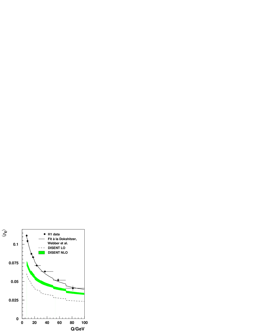
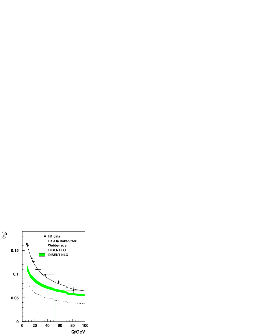
Abbildung 10.3: Corrected means (full symbols) of $\tau_{P}$, $B_{P}$, $\rho_{E}$ and $\tau_{C}$ as a function of $Q$. The error bars represent statistical uncertainties only. The full line corresponds to a power correction fit according to eqs. (10.9) and (10.21). For comparison the LO (dashed) and NLO (band) predictions of DISENT 0.1 are shown. The band reflects a variation of the renormalization scale of $1/2\leq\mu_{\scriptscriptstyle R}^{2}/\,{\rm GeV}^{2}\leq 2$.

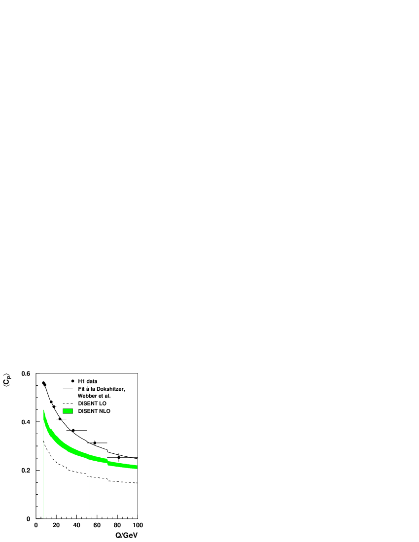
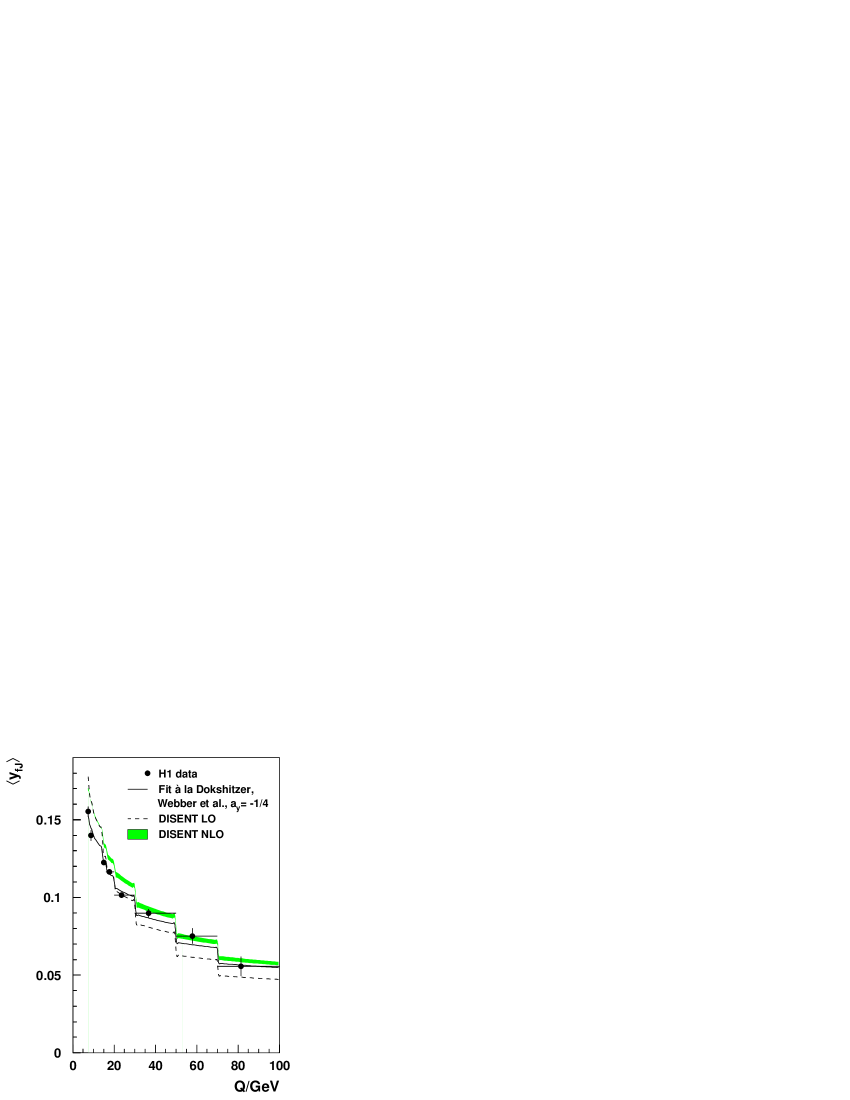
Abbildung 10.4: Corrected means (full symbols) of $C_{P}$, $y_{fJ}$ and $y_{k_{t}}$ as a function of $Q$. The error bars represent statistical uncertainties only. The full line corresponds to a power correction fit according to eqs. (10.9) and (10.21) except for $y_{k_{t}}$ where no power contribution was assumed. For comparison the LO (dashed) and, if appropriate, NLO (band) predictions of DISENT 0.1 are shown. The band reflects a variation of the renormalization scale of $1/2\leq\mu_{\scriptscriptstyle R}^{2}/\,{\rm GeV}^{2}\leq 2$.

Figs. 10.3 and 10.4 show the fit results in comparison with the corrected data as well as the LO and NLO predictions of DISENT 0.1 with respect to each corresponding $\alpha_{s}(M_{Z})$. The NLO band represents a variation of the renormalization scale of $1/2\leq\mu_{\scriptscriptstyle R}^{2}/\,{\rm GeV}^{2}\leq 2$, s. section 10.5 for details. Each fit taken separately, the data are nicely described. Putting all five in terms of $(\alpha_{s},\overline{\alpha}_{0})$-pairs into the one fig. 10.5, the discussed discrepancies become obvious. But recall again that systematic uncertainties are treated individually and therefore only statistical uncertainties are included!

With $y_{fJ}$, one obtains a good fit but rather low numbers for $\overline{\alpha}_{0}(\mu_{\scriptscriptstyle I}=2\,{\rm GeV})$ and $\alpha_{s}(M_{Z})$, leading to the conclusion that the coefficient $a_{y_{fJ}}$ given in the proceedings [24] may not be appropriate. Referring back to section 10.2, $y_{fJ}$ does exhibit smaller hadronization corrections than thrust. The curve in fig. 10.4 was produced with $a_{y_{fJ}}=-1/4$ derived in section 10.4.3.

Concerning $y_{k_{t}}$, the coefficient $a_{y_{k_{t}}}$ is not known and the $1^{\dagger}$ in table 10.3 is pure guesswork. The fit for $p=1$ works not very well supporting the conjecture of a $1/Q^{2}$-term instead of $1/Q$. In fact, both results obtained with $p=2$ look more reasonable. Nevertheless, fig. 10.4 contains the outcome according to eq. (10.9) without any power correction.

Abbildung 10.5: Results of the two-parameter fits à la Dokshitzer, Webber et al. for the means of $\tau_{P}$, $B_{P}$, $\rho_{E}$, $\tau_{C}$ and $C_{P}$ in the form of $1\sigma$- and $2\sigma$-contours in the $(\alpha_{s},\overline{\alpha}_{0})$-plane for statistical uncertainties only.

10.4.2 Combined Fits

Based on QCD, the universality of $\alpha_{s}$ is on firm theoretical grounds. Not so, however, $\overline{\alpha}_{0}$ since here additional assumptions are made. It was therefore checked if fits allowing for different $\overline{\alpha}_{0}$’s are possible while enforcing one $\alpha_{s}(M_{Z})$. Correlations between the observables were ignored for that purpose. According to the systematic behaviour found previously concerning the $\alpha_{s}(M_{Z})$-results, several combinations are tried. The outcome is collected in table 10.4.

The first two arrangements reflect the separation in $\tau_{P}$, $B_{P}$ on the one hand, and $\rho_{E}$, $\tau_{C}$, $C_{P}$ on the other. As expected, the numbers show resemblance to what we have obtained before. Yet, including step by step first $\tau_{P}$ and then $B_{P}$ into the $\rho_{E}$, $\tau_{C}$, $C_{P}$ triple, the $\chi^{2}/{\rm dof}$-values worsen considerably. Both times the fit results are dominated by the latter, which in addition to be more numerous, also have the smaller statistical uncertainties. $\alpha_{s}(M_{Z})$ is forced to remain high, and thereby $\overline{\alpha}_{0}(\mu_{\scriptscriptstyle I}=2\,{\rm GeV})$ for $\tau_{P}$ and $B_{P}$ is shifted.

One concludes that combined fits with one $\alpha_{s}(M_{Z})$ are possible, but notwithstanding the freedom to choose an individual $\overline{\alpha}_{0}$ for each event shape, they suffer from systematic effects. In order to determine $\alpha_{s}(M_{Z})$, it would be interesting to know what their origin is and what biases are implied.

Comb. fits:	$\tau_{P}$, $B_{P}$	$\rho_{E}$, $\tau_{C}$, $C_{P}$	$\tau_{P}$, $\rho_{E}$, $\tau_{C}$, $C_{P}$	$\tau_{P}$, $B_{P}$, $\rho_{E}$, $\tau_{C}$, $C_{P}$
$\overline{\alpha}_{0}(\tau_{P})$	$0.532\pm 0.012$	—	$0.374\pm 0.010$	$0.414\pm 0.009$
$\overline{\alpha}_{0}(B_{P})$	$0.488\pm 0.005$	—	—	$0.443\pm 0.006$
$\overline{\alpha}_{0}(\rho_{E})$	—	$0.561\pm 0.004$	$0.561\pm 0.004$	$0.562\pm 0.004$
$\overline{\alpha}_{0}(\tau_{C})$	—	$0.476\pm 0.003$	$0.476\pm 0.003$	$0.474\pm 0.003$
$\overline{\alpha}_{0}(C_{P})$	—	$0.428\pm 0.002$	$0.427\pm 0.002$	$0.421\pm 0.002$
$\alpha_{s}(M_{Z})$	$0.1115\pm 0.0011$	$0.1291\pm 0.0007$	$0.1285\pm 0.0007$	$0.1245\pm 0.0006$
$\chi^{2}/{\rm dof}$	$11.6/13$	$38.4/20$	$55.5/27$	$222/34$

Tabelle 10.4: Results of combined fits à la Dokshitzer, Webber et al. allowing for a separate $\overline{\alpha}_{0}(\mu_{\scriptscriptstyle I}=2\,{\rm GeV})$ for each event shape, but enforcing one $\alpha_{s}(M_{Z})$. Several combinations are tried; uncertainties are statistical only.

10.4.3 $\char 97\relax_{F}$-Fits

Motivated by the problems encountered with the $a_{F}$-coefficients for the $y$ event shapes, one can try to do a three-parameter fit of $\overline{\alpha}_{0}$, $\alpha_{s}(M_{Z})$ and $a_{F}$. However, this set of parameters is strongly correlated and with eight data points only it does not properly converge for $\tau_{P}$, $B_{P}$, $\rho_{E}$, $\tau_{C}$ or $C_{P}$. The $y$ variables are somewhat of an exception here, giving $\overline{\alpha}_{0}(\mu_{\scriptscriptstyle I}=2\,{\rm GeV})=0.58\pm 0.20$, $\alpha_{s}(M_{Z})=0.134\pm 0.015$ and $a_{y_{fJ}}=-0.71\pm 0.18$ at $\chi^{2}/{\rm dof}=1.6$ for $y_{fJ}$, and $\overline{\alpha}_{1}(\mu_{\scriptscriptstyle I}=2\,{\rm GeV})=0.35\pm 0.05$, $\alpha_{s}(M_{Z})=0.123\pm 0.006$ and $a_{y_{k_{t}}}=-33.2\pm 3.0$ at $\chi^{2}/{\rm dof}=0.23$ for $y_{k_{t}}$ respectively. Despite looking quite reasonable, one nevertheless has to exercise caution because of the very strong correlations.

Being constrained that way to less than three parameters, we start from the other side by deriving $a_{F}$ while presupposing the validity of eq. 10.21 with $\overline{\alpha}_{0}(\mu_{\scriptscriptstyle I}=2\,{\rm GeV})=0.5$ and $\alpha_{s}(M_{Z})=0.119$. Table 10.5 compiles the determined coefficients, which, although some rather large $\chi^{2}/{\rm dof}$’s occur, are of a similar magnitude as the theoretical ones. Notably, $y_{fJ}$ gives $a_{F}\approx-1/4$ instead of $1$!

As a consistency check, this new value was reinserted to produce the two-parameter fit in fig. 10.4 with $\overline{\alpha}_{0}(\mu_{\scriptscriptstyle I}=2\,{\rm GeV})=0.46$ and $\alpha_{s}(M_{Z})=0.118$, s. again table 10.3. Performing the same, i.e. $p=1$, circular procedure with $y_{k_{t}}$, one gets $\overline{\alpha}_{0}(\mu_{\scriptscriptstyle I}=2\,{\rm GeV})=0.34$ and $\alpha_{s}(M_{Z})=0.112$ which looks much better than the entry in table 10.3, but still is not satisfactory. Since $\overline{\alpha}_{1}$ is basically unknown, we must determine it in addition to $a_{F}$ in case of $p=2$. Refitting then with $a_{F}=-30$, one obtains $\overline{\alpha}_{1}(\mu_{\scriptscriptstyle I}=2\,{\rm GeV})=0.33$ and $\alpha_{s}(M_{Z})=0.121$, s. table 10.3. Both refits, however, exhibited strong correlations between $\overline{\alpha}_{0}$ respectively $\overline{\alpha}_{1}$ and $\alpha_{s}(M_{Z})$.

In a last test, all coefficients were multiplied by factors of $2$ respectively $1/2$ to study the effect on the $\overline{\alpha}_{0}(\mu_{\scriptscriptstyle I}=2\,{\rm GeV})$, $\alpha_{s}(M_{Z})$ results. Having fig. 10.5 in mind, the outcome corresponds approximately to shifts along the main diagonal with large $a_{F}$’s inducing smaller $\overline{\alpha}_{0}(\mu_{\scriptscriptstyle I}=2\,{\rm GeV})$’s and $\alpha_{s}(M_{Z})$’s.

$F$	$a_{F}$	$\chi^{2}/{\rm dof}$	$F$	$a_{F}$	$\chi^{2}/{\rm dof}$	$F$	$a_{F}$	$\chi^{2}/{\rm dof}$
$\tau_{P}$	$0.84\pm 0.03$	$0.4$	$\rho_{E}$	$0.65\pm 0.01$	$11.2$	$y_{fJ}$	$-0.23\pm 0.01$	$1.3$
$B_{P}$	$0.41\pm 0.01$	$6.0$	$\tau_{C}$	$0.88\pm 0.01$	$9.0$	$y_{k_{t}}$	$-0.41\pm 0.02$	$1.8$
			$C_{P}$	$2.85\pm 0.04$	$27.7$

Tabelle 10.5: Results for fits of the coefficients $a_{F}$ while presupposing the validity of eq. 10.21 with $\overline{\alpha}_{0}(\mu_{\scriptscriptstyle I}=2\,{\rm GeV})=0.5$ and $\alpha_{s}(M_{Z})=0.119$. Uncertainties are statistical only.

10.5 Evaluation of Systematic Uncertainties

The general procedure followed here is to repeat the fits for a variation in every prominent origin of systematic effects. The obtained discrepancy compared to the standard result is attributed to a corresponding uncertainty. In case of two deviations in one direction for the same primary source, e.g. an up- and downwards modification of an energy scale, only the larger one is considered for the evaluation of the total uncertainty. The latter is derived from all contributions by adding them up quadratically. An exception is the unfolding, whose influence is estimated in the same way as explained in section 7.5 on the final results of the data means.

Altogether, the following studies have been performed to estimate systematic effects:

• Experimental uncertainties:

  1. Usage of four unfolding procedures

  2. Variation of the electromagnetic energy scale of the calorimeters by $\pm 1\%$, $2\%$, $3\%$ depending on $z_{\rm imp}$

  3. Variation of the hadronic energy scale of the LAr calorimeter by $\pm 4\%$

• Theoretical uncertainties:

  1. Variation of the renormalization scale $\mu_{\scriptscriptstyle R}^{2}=Q^{2}$ by factors of $2$ and $1/2$

  2. Variation of the factorization scale $\mu_{\scriptscriptstyle F}^{2}=Q^{2}$ by factors of $4$ and $1/4$

  3. Variation of the infrared matching scale $\mu_{\scriptscriptstyle I}$ by $\pm 1/2\,{\rm GeV}$

  4. Selection of the MRSA’-105 and MRSA’-130 pdfs [62] with lower respectively higher intrinsic $\alpha_{s}(M_{Z})$ than in the standard pdfs

  5. Usage of the completely different pdf set CTEQ4A2 [85] with similar $\alpha_{s}(M_{Z})$

The experimental sources have already been described in section 7.5, but concerning the theoretical ones, some remarks are in order. The renormalization scale $\mu_{\scriptscriptstyle R}$ as well as the factorization scale $\mu_{\scriptscriptstyle F}$ (s. [50] for details) are arbitrary in the sense that in a complete theory the calculations are not allowed to vary with any specific choice. Yet, in reality we have only an approximative theory at our disposal yielding residual dependences due to the neglected higher orders. To avoid the appearance of large logarithms in the computations, it is recommended to identify them with a process relevant scale which for our purposes is always $Q$. To estimate the effect of omitted higher orders, it is conventional to vary them by an arbitrary factor of $4$ concerning the squares $\mu_{\scriptscriptstyle R}^{2}$, $\mu_{\scriptscriptstyle F}^{2}$. In the case of $\mu_{\scriptscriptstyle R}^{2}$, we had to reduce this factor to $2$ because of the condition (10.14): $\Lambda\ll\mu_{\scriptscriptstyle I}\approx 2\,{\rm GeV}\ll Q$. Taking this into account, varied results can be achieved quickly via eq. (8.21). With respect to $\mu_{\scriptscriptstyle F}$, however, the complete calculations have to be redone.

The change of the infrared matching scale $\mu_{\scriptscriptstyle I}$ by $\pm 1/2$ follows from the values used in the original proposal [6]. Note that this contributes only to the uncertainty for $\alpha_{s}(M_{Z})$! $\overline{\alpha}_{0}$ explicitly depends on $\mu_{\scriptscriptstyle I}$.

The next point accounts for the fact that implicitly $\alpha_{s}(M_{Z})$ has already been used in deriving the pdfs from data which in turn may bias our computations. The same is true for the choice of parameterization of the pdfs. For those reasons, three alternative sets, two with different assumptions on $\alpha_{s}(M_{Z})$ and one with approximately the same $\alpha_{s}(M_{Z})$ but another parameterization, have been selected for a reevaluation with DISENT 0.1.

All uncertainties described are presented graphically in figs. 10.6–10.8, separately for each of the five event shapes where the coefficients $a_{F}$ are known. Without such a prediction for $y_{fJ}$ and $y_{k_{t}}$, a study of systematic effects is omitted.

Abbildung 10.6: Systematic uncertainties of $\overline{\alpha}_{0}(\mu_{\scriptscriptstyle I}=2\,{\rm GeV})$ (left) and $\alpha_{s}(M_{Z})$ (right) for $\tau_{P}$ (top) and $B_{P}$ (bottom).

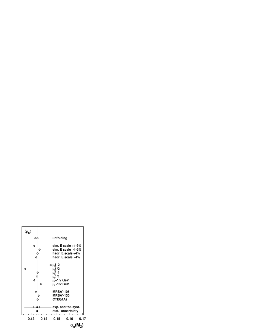
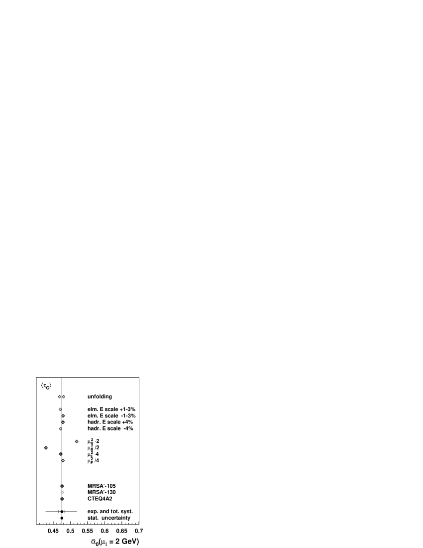
Abbildung 10.7: Systematic uncertainties of $\overline{\alpha}_{0}(\mu_{\scriptscriptstyle I}=2\,{\rm GeV})$ (left) and $\alpha_{s}(M_{Z})$ (right) for $\rho_{E}$ (top) and $\tau_{C}$ (bottom).

Abbildung 10.8: Systematic uncertainties of $\overline{\alpha}_{0}(\mu_{\scriptscriptstyle I}=2\,{\rm GeV})$ (left) and $\alpha_{s}(M_{Z})$ (right) for $C_{P}$.

Inspecting the figs. 10.6–10.8 again, it stands out that $\tau_{P}$ and $B_{P}$ behave differently compared to $\rho_{E}$, $\tau_{C}$ and $C_{P}$. For the latter, the systematic uncertainties are clearly dominated by the variation of the renormalization scale. In case of $\tau_{P}$ and $B_{P}$, this is much less pronounced. The larger influence of experimental uncertainties probably can be related to the explicit reference to the boson axis implied in the definitions of $\tau_{P}$ and $B_{P}$.

10.6 Cross-Checks

Concerning systematic effects some additional cross-checks were performed:

1. In order to ensure a reliable measurement of the scattered electron, partially inefficient regions between calorimeter modules ($\phi$-cracks) or wheels ($z$-cracks) are avoided. This selectively diminishes the contribution to certain phase space regions and is corrected for by the procedure described in section 7.2. Nevertheless, it was checked that the actual influence is negligible, even without unfolding.

2. The derivation of the power correction coefficients does not account for phase space constraints such as the cuts nos. • ‣ 5.5 and • ‣ 5.5 imposed on the scattered electron. Experimentally, they are absolutely necessary, but for testing purposes the NLO calculations were repeated without these cuts. Except for $\left<y_{k_{t}}\right>$, which increased by about $8\%$ in the low $Q^{2}$ region, all other mean values changed by less than $2\%$.

Kapitel 11 Summary and Outlook

The first measurement of event shapes in $ep$ DIS [25, 23], covering a range in $Q$ from $7\,{\rm GeV}$ up to $100\,{\rm GeV}$ in a single experiment, has been substantially improved and extended to include the additional variables $\rho_{E}$, $C_{P}$, $y_{fJ}$ and $y_{k_{t}}$ as well as new data taken in $1997$. The available statistics in the high $Q^{2}$ sample was more than doubled, facilitating a bisection of the highest $Q$-bin. The improvements encompass i.a. a more precise calibration of the energy of the scattered electron, an unfolding of the data distributions applying a Bayesian approach and a full account of radiative QED corrections. Taking into consideration the predominant sources of systematic influences, i.e. the accuracy of the electromagnetic and hadronic energy scale of the calorimeters and the unfolding procedure, corrected mean values of the event shape spectra together with estimates on their statistical and systematic uncertainty could be derived.

All event shape means exhibit a strong $Q$-dependence. They decrease with rising $Q$, i.e. the energy flow becomes more collimated. For the event shapes defined in the current hemisphere alone, it is interesting to compare with corresponding ones in $e^{+}e^{-}$ collisions. This was already done in [23] for $\left<\tau_{C}\right>$ and $\left<\tau_{P}\right>$ as well as $\left<\rho_{Q}\right>$. Despite the fact that the QCD dynamics in $ep$ DIS is different, a large similarity not only in the $Q$-dependence, but also in absolute value to their $e^{+}e^{-}$ counterparts could be established. When consulting reanalyzed data of the JADE Collaboration [87], this still holds for the $C$ parameter, but not for the jet broadening. $B_{P}$ is about a factor two larger than the wide as well as the total jet broadening.

Employing calculations in pQCD to NLO accuracy, the influence of parton fragmentation and hadronization could be studied. As an improvement, the approximative treatment of the $x$-dependence of the perturbative coefficients applied in [23] has been replaced by a more precise bin-wise evaluation. A direct comparison with data revealed that the investigated event shapes can roughly be categorized into three classes:

1. The event shapes $\tau_{P}$ and $B_{P}$ employing the $z^{\star}$-axis as event axis are sensitive to QED radiation. They show hadronization corrections of medium size.

2. $\rho_{E}$, $\tau_{C}$ and $C_{P}$ are strongly affected by the non-perturbative transition to hadrons. Their by far largest systematic uncertainty is due to the variation of the renormalization scale $\mu_{\scriptscriptstyle R}$.

3. Both event shapes based on jet algorithms, $y_{fJ}$ and $y_{k_{t}}$, exhibit small (even negative) hadronization corrections.

Fixing $\alpha_{s}(M_{Z})$ to $0.119$, the current world average [5], simple power corrections $\lambda/Q$ and $\mu/Q^{2}$ to parameterize the discrepancies between data and theory were tested. For $\lambda$, reasonable results of $0.7\,{\rm GeV}$ and $0.5\,{\rm GeV}$ could be obtained for $\tau_{P}$ and $B_{P}$, whereas $y_{fJ}$ and $y_{k_{t}}$ yielded negative values of $-0.2\,{\rm GeV}$ and $-0.4\,{\rm GeV}$ respectively. For the other event shapes the fit delivered poor $\chi^{2}/{\rm dof}$’s. This is generally the case for $\mu/Q^{2}$-terms; except for maybe $y_{fJ}$ and $y_{k_{t}}$, they are ruled out. Fitting $\alpha_{s}(M_{Z})$ in addition to $\lambda$ or $\mu$ did not help either due to very large correlations.

Invoking the approach for power corrections initiated by Dokshitzer and Webber, the situation improves significantly. For $\tau_{P}$, $B_{P}$, $\rho_{E}$, $\tau_{C}$ and $C_{P}$, where predictions for the coefficients $a_{F}$ are available, correlations were reduced — although not as far as desirable — and the fits converged nicely. Note that for $B_{P}$ the new coefficient $a^{\prime}_{B_{P}}$ replacing the formerly predicted logarithmic term had to be included. Within $20\%$, all determined $\overline{\alpha}_{0}$’s are compatible with a universal value of $\overline{\alpha}_{0}(\mu_{\scriptscriptstyle I}=2\,{\rm GeV})\approx 0.5$. Very similar results are achieved with this model when applied to $e^{+}e^{-}$ data [87, 88, 89] except for the wide jet broadening.

Concerning $\alpha_{s}(M_{Z})$, an inconvenient spread ranging from $0.111$–$0.135$ is observed. Although all five values turned out to be consistent with each other, a simple averaging seems to be inappropriate since the outcomes for $\alpha_{s}(M_{Z})$ again reflect two of the categories defined above. $\tau_{P}$ and $B_{P}$ mark the lower bound of the range in $\alpha_{s}(M_{Z})$ as opposed to $\rho_{E}$, $\tau_{C}$ and $C_{P}$ at the upper end. Combining several of these event shapes, the fits did work, but their quality severely declined, even allowing an individual $\overline{\alpha}_{0}$ for each. As long as this systematic behaviour is not better understood, a precise determination of $\alpha_{s}(M_{Z})$ is not feasible that way. Derived from the spread above, it can be stated at best that $\alpha_{s}(M_{Z})=0.123\pm 0.012$.

Returning to the $y$ event shapes, the conjectured coefficient of $a_{y_{fJ}}=1$ has been excluded. Derived from data keeping $\overline{\alpha}_{0}(\mu_{\scriptscriptstyle I}=2\,{\rm GeV})=0.5$ and $\alpha_{s}(M_{Z})=0.119$ fixed, a value of about $-1/4$ can be predicted. Without any coefficient given for $y_{k_{t}}$, it can only be checked for the power $p$ of the $1/Q^{p}$ term. Due to the smallness of the observed hadronization corrections in comparison with experimental uncertainties, however, it is very difficult to extract them from data. In fact, the performed investigations hint at powers $p>1$, but they are not conclusive enough to claim more.

The achieved measurements can be complimented in several ways:

• Instead of looking for the $Q$-dependence alone, the data could additionally be divided into bins in $x$. This is done by the ZEUS Collaboration [86].

• In $e^{+}e^{-}$ annihilation the model of Dokshitzer and Webber et al. has been extended to differential distributions [78, 76]. Although no predictions for $ep$ DIS exist, it is straightforward to just look what comes out, since the unfolded event shape spectra are at hand. Actually, a first check was already performed [49] and revealed inconsistencies even between fits of the mean values and distributions of one shape variable. Resummed calculations which are not available for $ep$ DIS may be helpful.

• By further subdividing a distribution into intervals as done by the DELPHI Collaboration, it is possible to examine where specific power-like contributions occur [89, 90].

• Alternatively, higher moments of already investigated event shapes can be studied. First steps into that direction were taken by the OPAL Collaboration [91].

• Another obvious extension is the usage of new variables, possibly with small hadronization corrections.

Especially concerning the last point, however, the question arises of what to do with them. For $y_{k_{t}}$ it was already noticed that with the given experimental uncertainties power contributions can not be reliably extracted. Yet, just in this case it could be interesting to perform direct fits of $\alpha_{s}(M_{Z})$ with the distributions at high $Q^{2}$. Remaining hadronization corrections must then be estimated by the usual procedure of correcting to the parton level of MC models. At the same time, this could be done for the event shapes of this analysis, such that a comparison of the fit results in $\alpha_{s}(M_{Z})$ could provide insight into systematic effects in one (or both) of these methods.

At last, it should be mentioned that the per se sharp angular cut-off of $90{{}^{\circ}}$ in the Breit frame is neither theoretically nor experimentally unproblematic, (s. sections 4.2 and 5.5). It has been suggested to replace it by a kind of weighting procedure to ensure a smooth transition. On the other hand, one could try to separate the remnant by employing e.g. the $k_{t}$-algorithm and treat then all remaining objects as input for the derivation of event shapes.

Abbildungsverzeichnis

1. 2.1 The storage ring HERA at the DESY laboratory in Hamburg, Germany.
2. 2.2 Schematic layout of the H1 detector.
3. 2.3 The layout of the H1 luminosity system.
4. 2.2.2 Details on the Main Components
5. 3.1 Diagram of the basic $ep$ DIS process via neutral currents.
6. 3.2 Lines of constant energy and polar angle for the scattered electron and the current jet in the $(x,Q^{2})$-plane.
7. 3.3 Quark-Parton-Model Feynman graph and a virtual correction to it.
8. 3.4 QCD-Compton Feynman graphs.
9. 3.5 Boson-Gluon-Fusion Feynman graphs.
10. 4.1 Example of an $ep$ collision measured with the H1 detector.
11. 4.2 Diagram of a QPM-type $ep$ collision as seen in the Breit frame.
12. 4.3 Polar angles and energies in the Breit frame in dependence of energy and angles of a four-vector in the laboratory system.
13. 4.4 $(x_{p},z_{p})$ phase space region for ${\cal O}(\alpha_{s})$ corrections to DIS.
14. 5.1 Integrated luminosity produced and accumulated during the running periods from $1992$ up to $1997$.
15. 5.2 A principal diagram of the data stream in H1.
16. 5.3 Distribution of finally selected events in the $(x,Q^{2})$-plane.
17. 5.4 Number of selected events in 1994 and the rate of selected events from 1994–1997 versus the integrated luminosity.
18. 6.1 ${\cal O}(\alpha)$ real corrections to the QPM Feynman graph.
19. 6.2 Normalized differential distributions of $C_{P}$ on cluster level compared with LEPTO 6.5 and HERWIG 5.8.
20. 6.3 Normalized differential distributions of $E_{e^{\prime}}$, $\theta_{e^{\prime}}$ and $\ln(Q_{e}^{2}/\,{\rm GeV}^{2})$ on cluster level.
21. 6.4 Normalized differential distributions of $y_{h}$, $(E-P_{z})$ and $\theta_{q}$ on cluster level.
22. 6.5 Normalized differential distributions of $\tau_{P}$, $B_{P}$, $\rho_{E}$ and $\tau_{C}$ on cluster level.
23. 6.6 Normalized differential distributions of $C_{P}$, $y_{fJ}$ and $y_{k_{t}}$ on cluster level.
24. 7.1 Bin-wise detector corrections for $\tau_{P}$, $B_{P}$, $\rho_{E}$ and $\tau_{C}$.
25. 7.2 Bin-wise detector corrections for $C_{P}$, $y_{fJ}$ and $y_{k_{t}}$.
26. 7.3 Correlation matrices for $\tau_{P}$, $B_{P}$ and $\rho_{E}$.
27. 7.4 Correlation matrices for $\tau_{C}$, $C_{P}$ and $y_{fJ}$.
28. 7.5 Correlation matrices for $y_{k_{t}}$.
29. 7.6 Bin-wise radiative corrections for $\tau_{P}$, $B_{P}$, $\rho_{E}$ and $\tau_{C}$.
30. 7.7 Bin-wise radiative corrections for $C_{P}$, $y_{fJ}$ and $y_{k_{t}}$.
31. 7.8 Means of $C_{P}$ and $\tau_{P}$ as a function of $Q$ for simulated event samples corrected with a second MC to check the unfolding procedure.
32. 7.9 Unfolded means of $\tau_{P}$, $B_{P}$, $\rho_{E}$ and $\tau_{C}$ as a function of $Q$ for four correction schemes.
33. 7.10 Unfolded means of $C_{P}$, $y_{fJ}$ and $y_{k_{t}}$ as a function of $Q$ for four correction schemes.
34. 7.11 Corrected means of $\tau_{P}$, $B_{P}$, $\rho_{E}$ and $\tau_{C}$ as a function of $Q$.
35. 7.12 Corrected means of $C_{P}$, $y_{fJ}$ and $y_{k_{t}}$ as a function of $Q$.
36. 8.1 Examples of real corrections to QCDC and BGF Feynman graphs.
37. 8.2 Examples of 2-loop virtual correction Feynman graphs.
38. 8.3 Differential distributions of $\tau_{P}$ at LO and NLO for MEPJET 1.4 and DISENT 0.0.
39. 9.1 Histograms of $\sigma_{\rm tot}$ and $\left<\tau_{P}\right>$ resulting from repeated DISENT 0.0 calculations and the dependence of their statistical uncertainties on $1/\sqrt{N}$.
40. 9.2 Mean values of $\tau_{P}$ and $C_{P}$ versus $Q$ in four different bins of $x$.
41. 9.3 Fits of $\Lambda_{5,\overline{\rm MS}}$ for the LO and NLO means of $\tau_{P}$ and $C_{P}$.
42. 10.1 Normalized differential distributions of $\tau_{P}$, $B_{P}$, $\rho_{E}$ and $\tau_{C}$ corrected to hadron level in comparison with NLO predictions.
43. 10.2 Normalized differential distributions of $C_{P}$, $y_{fJ}$ and $y_{k_{t}}$ corrected to hadron level in comparison with NLO predictions.
44. 10.3 Power correction fits to corrected means of $\tau_{P}$, $B_{P}$, $\rho_{E}$ and $\tau_{C}$ together with the LO and NLO predictions.
45. 10.4 Power correction fits to corrected means of $C_{P}$ and $y_{fJ}$ and a fit without power correction to the corrected means of $y_{k_{t}}$, together with the LO and NLO predictions.
46. 10.5 Results of the two-parameter fits à la Dokshitzer, Webber et al. for the means of $\tau_{P}$, $B_{P}$, $\rho_{E}$, $\tau_{C}$ and $C_{P}$ in the $(\alpha_{s},\overline{\alpha}_{0})$-plane.
47. 10.6 Systematic uncertainties of $\overline{\alpha}_{0}(\mu_{\scriptscriptstyle I}=2\,{\rm GeV})$ and $\alpha_{s}(M_{Z})$ for $\tau_{P}$ and $B_{P}$.
48. 10.7 Systematic uncertainties of $\overline{\alpha}_{0}(\mu_{\scriptscriptstyle I}=2\,{\rm GeV})$ and $\alpha_{s}(M_{Z})$ for $\rho_{E}$ and $\tau_{C}$.
49. 10.8 Systematic uncertainties of $\overline{\alpha}_{0}(\mu_{\scriptscriptstyle I}=2\,{\rm GeV})$ and $\alpha_{s}(M_{Z})$ for $C_{P}$.

Tabellenverzeichnis

1. 4.1 Formulae for the event shapes in ${\cal O}(\alpha_{s})$.
2. 4.2 Upper bounds for the defined event shapes.
3. 5.1 Cross sections and rates at design luminosity.
4. 5.2 Final phase space cuts.
5. 5.3 Final data quality cuts.
6. 5.4 Integrated luminosities and events gathered in the selection steps.
7. 6.1 Cluster level MC statistics.
8. 6.2 Uncorrected mean values of the event shapes as a function of $Q$.
9. 7.1 Corrected mean values of the event shapes as a function of $Q$.
10. 9.1 Mean $Q$- and $x$-values as well as the LO and NLO cross sections.
11. 9.2 Mean values and perturbative coefficients for $\tau_{P}$.
12. 9.3 Mean values and perturbative coefficients for $B_{P}$.
13. 9.4 Mean values and perturbative coefficients for $\rho_{E}$.
14. 9.5 Mean values and perturbative coefficients for $\tau_{C}$.
15. 9.6 Mean values and perturbative coefficients for $C_{P}$.
16. 9.7 Mean values and perturbative coefficients for $y_{fJ}$.
17. 9.8 Mean values and perturbative coefficients for $y_{k_{t}}$.
18. 10.1 Results of one-parameter fits without power corrections and according to the tube model.
19. 10.2 Results of two-parameter fits according to the tube model.
20. 10.3 Results of two-parameter fits à la Dokshitzer, Webber et al.
21. 10.4 Results of combined fits à la Dokshitzer, Webber et al.
22. 10.5 Results for fits of the coefficients $a_{F}$ of the model of Dokshitzer, Webber et al.

Curriculum Vitae

Geburtsdatum:	13. Januar 1967
Geburtsort:	Mönchengladbach
Familienstand:	ledig
Staatsangehörigkeit:	deutsch
Eltern:	Matthias Rabbertz, Weber
	Gertrud Rabbertz, geb. Hermanns, Bankangestellte
Geschwister:	Beate Reitler
	Gerda Boms

Schulbildung:	01.08.73 - 06.07.77	Gemeinschaftsgrundschule Wegberg
	01.08.77 - 12.06.86	Städtisches Maximilian-Kolbe-Gymnasium Wegberg Abschluß: Allgemeine Hochschulreife
Wehrdienst:	01.10.86 - 31.12.87	Grundausbildung in Pinneberg Tätigkeit als Sprechfunker in Geilenkirchen
Studium:	01.10.87 - 08.26.94	Rheinisch-Westfälische Technische Hochschule Aachen, Mathematisch-Naturwissenschaftliche Fakultät Studienfach: Physik Fachrichtung: Elementarteilchenphysik Abschluß: Diplom-Physiker
	01.11.89 - 15.10.92	Tätigkeit als studentische Hilfskraft am Institut für Mathematik, Prof. Dr. G. Hellwig
	seit 01.07.94	Wissenschaftlicher Angestellter am I. Physikalischen Institut der Rheinisch-Westfälischen Technischen Hochschule Aachen, Beginn des Promotionsvorhabens bei Prof. Dr. Ch. Berger
	seit 01.01.95	Mitglied der H1-Kollaboration am DESY, Hamburg