RIKEN-AF-NP-324, SAGA-HE-143-99
KOBE-FHD-99-03, FUT-99-02
 
 
 
Polarized Parton Distribution Functions in the Nucleon  
 

Abstract

Polarized parton distribution functions are determined by using world data from the longitudinally polarized deep inelastic scattering experiments. A new parametrization of the parton distribution functions is adopted by taking into account the positivity and the counting rule. From the fit to the asymmetry data $A_{1}$, the polarized distribution functions of $u$ and $d$ valence quarks, sea quarks, and gluon are obtained. The results indicate that the quark spin content is $\Delta\Sigma=$0.20 and 0.05 in the leading order (LO) and the next-to-leading-order (NLO) $\overline{\rm MS}$ scheme, respectively. However, if $x$ dependence of the sea-quark distribution is fixed at small $x$ by “perturbative QCD” and Regge theory, it becomes $\Delta\Sigma=0.24\sim 0.28$ in the NLO. The small-$x$ behavior cannot be uniquely determined by the existing data, which indicates the importance of future experiments. From our analysis, we propose one set of LO distributions and two sets of NLO ones as the longitudinally-polarized parton distribution functions.

PACS number(s): 13.60.Hb, 13.88.+e

I INTRODUCTION

For a long time, deep inelastic scattering (DIS) of leptons from the nucleon has served as an important tool for studying the nucleon substructure and testing the quantum chromodynamics (QCD). Structure functions of the nucleon have been measured with this reaction in great precision, which often provides a firm basis of a search for new physics in hadron collisions. In addition, basic parameters of QCD such as $\alpha_{s}$ or $\Lambda_{\rm QCD}$ have been obtained from the $Q^{2}$ dependence of the structure functions. Consequently, hadron-related reactions at high energies are described by the parton model and perturbative QCD with reasonable precision.

The measurement of the polarized structure function $g_{1}^{p}(x,Q^{2})$ by the European Muon Collaboration (EMC) in 1988 [1] has, however, revealed more profound structure of the proton, which is often referred to as ‘the proton spin crisis’. Their results are interpreted as very small quark contribution to the nucleon spin. Then, the rest has to be carried by the gluon spin and/or by the angular momenta of quarks and gluons. Another consequence from their measurement was that the strange quark is negatively polarized, which was not anticipated in a naive quark model.

The progress in the data precision is remarkable in post-EMC experiments. The final results of the Spin Muon Collaboration (SMC) experiment [2] have been reported, and its value of $A_{1}^{p}$ at the lowest $x$ has decreased in comparison with their previous one [3]. The final results of high-precision $A_{1}^{p}$ and $A_{1}^{d}$ data have been presented by the Stanford Linear Accelerator Center (SLAC) E143 collaboration [4], and they consist of more than 200 data points. Moreover, the measurement of $g_{1}^{p}(x,Q^{2})$ with the pure hydrogen target has been carried out by the HERMES collaboration [5]. In addition to such improvements in the data precision, new programs are underway or in preparation at SLAC, Brookhaven National Laboratory - Relativistic Heavy Ion Collider (BNL-RHIC)[6], European Organization for Nuclear Research (CERN) [7], etc., and results are expected to come out in the near future. On the other hand, theoretical advances such as the development of the next-to-leading-order (NLO) QCD calculations of polarized splitting functions [8, 9] stimulated many works on the QCD analysis of polarized parton distribution functions (PDFs) [10, 11, 12, 13, 14, 15, 16]. There is an attempt to obtain next-to-next-leading order (NNLO) splitting functions [17] and we can expect further progress in the precise analysis of polarized PDFs.

In this paper, we present an analysis of world data on the cross section asymmetry $A_{1}$ in the polarized DIS processes for the proton, neutron, and deuteron targets. We formed a group called Asymmetry Analysis Collaboration (AAC), and our goal is to determine polarized PDFs, $\Delta f_{i}(x,Q^{2})$, where $i=u,d,s,\bar{u},\bar{d},\bar{s},...,\,\,{\rm and}\ g$. Another possible approach is to parametrize structure functions, $g_{1}^{N}(x,Q^{2})$ ($N=p,n,{\rm and}~{}d$), which can be expressed as linear combinations of the PDFs. In the analysis and predictions of the cross section asymmetry in polarized hadron-hadron collisions, however, what we need are polarized PDFs rather than structure functions, because the contribution of each quark flavor is differently weighted in e.g. $gq\rightarrow gq$ from DIS where each flavor is weighted by electric charge squared.

We choose $A_{1}$ as the object of the analysis, since it is more close to the direct observable in experiments than $g_{1}^{N}(x,Q^{2})$. The $g_{1}^{N}(x,Q^{2})$ data published by the experiments depend on the knowledge on the unpolarized structure functions at the time of their publication. By choosing $A_{1}$ as the object of the analysis, we can extend the analysis to include new set of data easily without any change in the previous data set.

As explained in Sec. II, we parametrize the polarized parton distributions at small momentum transfer squared $Q^{2}=1.0$ GeV² ($\equiv Q_{0}^{2}$) with a special emphasis on the positivity and quark counting rule. Then, they are evolved to the $Q^{2}$ points, where the experimental data were taken, by the leading-order (LO) or NLO $Q^{2}$ evolution program. Using one of well-established unpolarized parton distributions, we construct $A_{1}$ as

$$A_{1}(x,Q^{2})\simeq\frac{g_{1}(x,Q^{2})}{F_{1}(x,Q^{2})},$$ (1)

to compare with the experimental data. The polarized parton distributions at the initial $Q_{0}^{2}$ are determined by a $\chi^{2}$ analysis.

In Sec. II, we describe the outline of our analysis with the necessary formulation and the data set used in the analysis. Section III is devoted to the explanation of the LO and NLO $Q^{2}$ evolution programs which we developed for our fit. The parametrization of the polarized parton distribution functions at the initial $Q_{0}^{2}$ is described in Sec. IV, and the fitting results are discussed in Sec. V. The conclusions are given in Sec. VI.

II PARTON MODEL ANALYSIS OF POLARIZED DIS DATA

In the experiments of polarized DIS, direct observables are the cross-section asymmetries $A_{\parallel}$ and $A_{\perp}$, which are defined as

$$A_{\parallel}=\frac{\sigma_{\downarrow\uparrow}-\sigma_{\uparrow\uparrow}}{\sigma_{\downarrow\uparrow}+\sigma_{\uparrow\uparrow}},~{}~{}~{}~{}~{}~{}~{}~{}A_{\perp}=\frac{\sigma_{\downarrow\rightarrow}-\sigma_{\uparrow\rightarrow}}{\sigma_{\downarrow\rightarrow}+\sigma_{\uparrow\rightarrow}}.$$ (2)

The $\sigma_{\uparrow\uparrow}$ and $\sigma_{\uparrow\downarrow}$ represent the cross sections for the lepton-nucleon scattering with their parallel and anti-parallel helicity states, respectively. On the other hand, the $\sigma_{\uparrow\rightarrow}$ and $\sigma_{\downarrow\rightarrow}$ are the scattering cross sections for transversely polarized nucleon target. We suppress the dependence on $x$ and $Q^{2}$ where it is evident hereinafter. The asymmetries, $A_{\parallel}$ and $A_{\perp}$, are related to the photon absorption cross section asymmetries, $A_{1}$ and $A_{2}$, by

$$A_{\parallel}={\cal D}(A_{1}+\eta A_{2}),~{}~{}~{}~{}A_{\perp}=d(A_{2}-\zeta A_{1}),$$ (3)

where ${\cal D}$ represents the photon depolarization factor and $\eta$ is approximated as $\gamma(1-y)/(1-y/2)$ with $\gamma=2Mx/\sqrt{Q^{2}}$. The $d$ and $\zeta$ are other kinematical factors. The asymmetries, $A_{1}$ and $A_{2}$, can be expressed as:

$$A_{1}(x,Q^{2})=\frac{\sigma_{T,\frac{1}{2}}-\sigma_{T,\frac{3}{2}}}{\sigma_{T,\frac{1}{2}}+\sigma_{T,\frac{3}{2}}}=\frac{g_{1}(x,Q^{2})-\gamma^{2}g_{2}(x,Q^{2})}{F_{1}(x,Q^{2})},$$ (4)

$$A_{2}(x,Q^{2})=\frac{2\sigma_{LT}}{\sigma_{T,\frac{1}{2}}+\sigma_{T,\frac{3}{2}}}=\frac{\gamma\,[g_{1}(x,Q^{2})+g_{2}(x,Q^{2})]}{F_{1}(x,Q^{2})}.$$ (5)

Here $\sigma_{T,\frac{1}{2}}$ and $\sigma_{T,\frac{3}{2}}$ are the absorption cross sections of virtual transverse photon for the total helicity of the photon-nucleon system of $\frac{1}{2}$ and $\frac{3}{2}$, respectively; $\sigma_{LT}$ is the interference term between the transverse and longitudinal photon-nucleon amplitudes; $F_{1}(x,Q^{2})$ is the unpolarized structure function of the nucleon. If we measure both $A_{\parallel}$ and $A_{\perp}$, we can extract both $g_{1}(x,Q^{2})$ and $g_{2}(x,Q^{2})$ from experimental data with minimal assumptions. Otherwise, $\eta A_{2}$ should be neglected in Eq. (3) to extract $A_{1}$. This is justified since $\eta A_{2}$ is much smaller than $A_{1}$ in the present kinematical region. However, its effect has to be included in the systematic error. In the small-$x$ or large-$Q^{2}$ region, $\gamma^{2}$ is the order of $10^{-3}-10^{-2}$. An absolute value of $g_{2}(x,Q^{2})$ has been measured to be significantly smaller than $g_{1}(x,Q^{2})$. Therefore, the asymmetry in Eq. (4) can be expressed by

$$A_{1}(x,Q^{2})\simeq\frac{g_{1}(x,Q^{2})}{F_{1}(x,Q^{2})},$$ (6)

to good approximation. Since the structure function usually extracted from unpolarized DIS experiments is $F_{2}(x,Q^{2})$, we use $F_{2}(x,Q^{2})$ instead of $F_{1}(x,Q^{2})$ by the relation

$$F_{1}(x,Q^{2})=\frac{F_{2}(x,Q^{2})}{2x[1+R(x,Q^{2})]}.$$ (7)

The function $R(x,Q^{2})$ represents the cross-section ratio for the longitudinally polarized photon to the transverse one, $\sigma_{L}/\sigma_{T}$, which is determined experimentally in reasonably wide $Q^{2}$ and $x$ ranges in the SLAC experiment of Ref. [18]. Recently published data on $R(x,Q^{2})$ by NMC[19] showed slightly different values from the SLAC measurement but mostly agreed within experimental uncertainties. Therefore, we decided to use SLAC measurements to be consistent with the most of the analyses of polarized DIS experiments.

The structure function $F_{2}$ can be written in terms of unpolarized PDFs with coefficient functions as

$$F_{2}(x,Q^{2})=\sum\limits_{i=1}^{n_{f}}e_{i}^{2}x\bigg{\{}C_{q}(x,\alpha_{s})\otimes[q_{i}(x,Q^{2})+\bar{q}_{i}(x,Q^{2})]+C_{g}(x,\alpha_{s})\otimes g(x,Q^{2})\bigg{\}}.$$ (8)

Here $q_{i}$ and $\bar{q}_{i}$ are the distributions of quark and antiquark of flavor $i$ with electric charge $e_{i}$. The gluon distribution is represented by $g(x,Q^{2})$. The convolution $\otimes$ is defined by

$$f(x)\otimes g(x)=\int^{1}_{x}\frac{dy}{y}f\left(\frac{x}{y}\right)g(y).$$ (9)

The coefficient functions, $C_{q}$ and $C_{g}$, are written as a series in $\alpha_{s}$ with $x$-dependent coefficients:

$$C(x,\alpha_{s})=\sum\limits_{k=0}^{\infty}\left(\frac{\alpha_{s}}{2\pi}\right)^{k}C^{(k)}(x).$$ (10)

The LO coefficient functions are simply given by

$$C_{q}^{(0)}(x)=\delta(1-x),~{}~{}~{}~{}C_{g}^{(0)}(x)=0.$$ (11)

In the same way, the polarized structure function $g_{1}(x,Q^{2})$ is expressed as

$$g_{1}(x,Q^{2})=\frac{1}{2}\sum\limits_{i=1}^{n_{f}}e_{i}^{2}\bigg{\{}\Delta C_{q}(x,\alpha_{s})\otimes[\Delta q_{i}(x,Q^{2})+\Delta\bar{q}_{i}(x,Q^{2})]+\Delta C_{g}(x,\alpha_{s})\otimes\Delta g(x,Q^{2})\bigg{\}},$$ (12)

where $\Delta q_{i}\equiv q^{\uparrow}_{i}-q^{\downarrow}_{i}$ ($i=u,d,s,...$) represents the difference between the number densities of quark with helicity parallel to that of parent nucleon and with helicity anti-parallel. The definitions of $\Delta\bar{q}_{i}$ and $\Delta g$ are the same. The polarized coefficient functions $\Delta C_{q}$ and $\Delta C_{g}$ are defined similarly to the unpolarized case.

Another separation of the quark distribution can be done by using flavor-singlet quark distribution $\Delta\Sigma(x,Q^{2})$ and flavor-nonsinglet quark distributions for the proton and the neutron, $\Delta q_{NS}^{p}(x,Q^{2})$ and $\Delta q_{NS}^{n}(x,Q^{2})$, respectively. Those can be expressed with polarized PDFs as follows:

$$\Delta\Sigma(x) = a_{0}(x)=\Delta u^{+}(x)+\Delta d^{+}(x)+\Delta s^{+}(x),$$ (13)

$$\Delta q_{NS}^{p,\,n}(x) = \pm\frac{3}{4}\,a_{3}(x)+\frac{1}{4}\,a_{8}(x)$$ (14)

$$= \pm\frac{3}{4}\,[\,\Delta u^{+}(x)-\Delta d^{+}(x)\,]+\frac{1}{4}\,[\,\Delta u^{+}(x)+\Delta d^{+}(x)-2\Delta s^{+}(x)\,],$$ (15)

where $\Delta u^{+}(x)=\Delta u(x)+\Delta\bar{u}(x)$ and similarly for $\Delta d^{+}(x)$ and $\Delta s^{+}(x)$. Analyses in Ref. [12] and Ref. [15] utilized this separation. Such separation is useful in $Q^{2}$ evolution, and it is also natural when one wants to obtain quark contribution to the proton spin, $\int_{0}^{1}\Delta\Sigma(x)dx$.

On the other hand, when we try to calculate the cross section for polarized $pp$ reaction, e.g. Drell-Yan production of lepton pairs, we need the combination of $\Delta q_{i}(x_{1})\times\Delta\bar{q}_{i}(x_{2})$ (multiplied by electric charge squared). To allow such calculations with the above separation, we need further assumption on the polarized antiquark distributions, e.g. flavor symmetric sea, $\Delta u_{\rm sea}(x)=\Delta\bar{u}(x)=\Delta d_{\rm sea}(x)=\Delta\bar{d}(x)=\Delta s(x)=\Delta\bar{s}(x)$. With such assumption, the above separation becomes equivalent to the PDF separation in a sense that one description can be translated to another by simple transformation.

Of course, we already know that unpolarized sea-quark distributions are not flavor symmetric [20] from various experiments including Drell-Yan production of lepton pairs in $pp$ and $pd$ collisions. Therefore, this assumption is only justified as an approximation due to limited experimental data. In principle, charged-hadron production data could clarify this issue. Although a $\chi^{2}$ analysis for the SMC and HERMES data seems to suggest a slight $\Delta\bar{u}$ excess over $\Delta\bar{d}$ [21], the present data are not accurate enough for finding such a flavor asymmetric signature. Future experiments with charged current at RHIC [22] and polarized option at HERA will be very useful in improving our knowledge on the spin-flavor structure of the nucleon. Furthermore, as it has been done in the unpolarized studies, the difference between the polarized $pp$ and $pd$ cross sections provides a clue for the polarized flavor asymmetry [23] although actual experimental possibility is uncertain at this stage.

The parametrization models studied so far have various differences in other aspects: (a) the choice of the renormalization scheme, (b) the functional form of the polarized parton distributions due to different physical requirements at $Q_{0}^{2}$, and (c) the physical quantity to be fitted. In the following, we describe our position on these issues.

• Renormalization Scheme
  Although the parton distributions have no scheme dependence in the LO, they do depend on the renormalization scheme in the NLO and beyond. In the polarized case, we have different choices of the scheme due to the axial anomaly and the ambiguity in treating the $\gamma_{5}$ in $n$ dimensions[16]. In the NLO analysis, the widely-used scheme is the modified minimal subtraction ($\overline{\rm MS}$) scheme, in which the first moment of the nonsinglet distribution is $Q^{2}$-independent. It was used, for example, by Mertig and van Neerven [8] and Vogelsang [9]. However, the first moment of the singlet distribution is $Q^{2}$-dependent in this scheme and thus it is rather difficult to compare the value of $\Delta\Sigma(x,Q^{2})$ extracted from the DIS at large $Q^{2}$ with the one from the static quark model at small $Q^{2}$. To cure this difficulty, Ball, Forte and Ridolfi [24] used the so-called AB (Adler-Bardeen) scheme, in which the first moment of the singlet distribution becomes independent of $Q^{2}$ because of the Adler-Bardeen theorem[25]. In those schemes, however, some soft contributions are included in the Wilson coefficient functions and not completely absorbed into the PDFs. Another scheme called the JET scheme [26] or the CI (chirally invariant) scheme [27] has been recently proposed. All the hard effects are absorbed into the Wilson coefficient functions in this scheme.

  Although we choose the $\overline{\rm MS}$ scheme in our analysis, the polarized PDFs in one scheme are related to those in other schemes with simple formulae [16].

• Functional Form of polarized PDF and Physical Requirements
  Different functional forms have been proposed so far for the polarized PDFs by taking account of various physical conditions. We choose the functional form with the special emphasis on the positivity condition and quark counting rule [28] at $Q^{2}_{0}=1.0$ GeV².

  The positivity condition is originated in a probabilistic interpretation of the parton densities. The polarized PDFs should satisfy the condition

  $$|\,\Delta f_{i}(x,Q^{2}_{0})\,|\leq f_{i}(x,Q^{2}_{0}).$$ (16)

  This is valid in the LO since we can have the complete probabilistic interpretation for each polarized distribution only at the LO. Even in NLO, however, the positivity condition for the polarized cross section $\Delta\sigma$ with the unpolarized cross section $\sigma$,

  $$|\,\Delta\sigma\,|\leq\sigma,$$ (17)

  should still apply for any processes to be calculated with the polarized PDFs to the order of ${\cal O}(\alpha_{s})$. Since it is very difficult to calculate the polarized and unpolarized cross sections of the NLO for all the possible processes, it is not realistic to determine the polarized NLO distributions by the positivity condition of Eq. (17). In our analysis, we simply require that Eq. (16) should be satisfied in the LO and also NLO at $Q_{0}^{2}$. It is shown in Ref. [29] that the NLO $Q^{2}$ evolution should preserve the positivity maintained at initial $Q^{2}_{0}$.

  In many cases, Regge behavior has been assumed for $x\rightarrow 0$, and the color coherence of gluon couplings has been also used at $x\simeq 0$ [30]. Furthermore, it is an interesting guiding principle that the polarized distributions have a similar behavior to the unpolarized ones in the large-$x$ region [16]. Since behavior of the distributions at large $x$ is determined by the term $(1-x)^{\beta}$ in the functions, where $\beta$ is a constant, we simply require that the polarized distributions should have the same $(1-x)^{\beta}$ term as the unpolarized ones.

  Those physical requirements and assumptions have to be tested by comparing with the existing experimental data.

  As for the choice of $Q_{0}^{2}$, it has to be large enough to apply perturbative QCD, but it should be small enough to maintain a large set of experimental data. We find $Q_{0}^{2}$=1.0 GeV² to be a reasonable choice in our analysis.

• Physical Quantities to be Fitted
  In most of the polarized experiments, the data have been presented for $A_{1}(x,Q^{2})$ and $g_{1}(x,Q^{2})$. Some analyses [12, 14, 15, 30] used the $g_{1}(x,Q^{2})$ as data samples, while others [10, 11, 13, 16] used the $A_{1}(x,Q^{2})$. It should be, however, noted that $g_{1}(x,Q^{2})$ is obtained by multiplying $A_{1}(x,Q^{2})$ by $F_{1}(x,Q^{2})$, so that it is not free from ambiguity of the unpolarized structure function, $F_{1}(x,Q^{2})$. Therefore, we consider that it is more advantageous to use the $A_{1}(x,Q^{2})$ as the data samples not only for the current work but also for the convenience in expanding the data set to include new data set from SLAC, DESY (German Electron Synchrotron), CERN, and RHIC.

  Another important quantity which we should carefully consider is the cross section ratio $R(x,Q^{2})=\sigma_{L}/\sigma_{T}$, where $\sigma_{L}$ and $\sigma_{T}$ are absorption cross sections of longitudinal and transverse photons, respectively. In principle, nonzero $R(x,Q^{2})$ is originated from radiative corrections in perturbative QCD, higher twist effects, and target mass effects. Higher twist contribution to $R(x,Q^{2})$ is expected to be small in the large $Q^{2}$ region. So far, some analyses employed nonzero $R(x,Q^{2})$, while other analyses assumed $R(x,Q^{2})=0$. However, the latter is not consistent with the experimental analysis procedure, since $R(x,Q^{2})$ is also used for the evaluation of photon depolarization factor ${\cal D}$. Indeed our analysis shows that world data prefer $R(x,Q^{2})\neq 0$: the $\chi^{2}$ increases significantly with $R=0$. Therefore, we use nonzero $R(x,Q^{2})$ in fitting the data of $A_{1}(x,Q^{2})$.

Table I summarizes experiments with published data on the polarized DIS [1, 2, 3, 4, 5, 31, 32, 33, 34]. These measurements cover a wide range of $x$ and $Q^{2}$ with various beam species and energies and various types of polarized nucleon target (not shown in the table). The listed are the number of data points above $Q^{2}=1.0$ GeV², and the total number of data points are 375.

We use the data with minimal manipulation to analyze them in our framework so as to be consistent with the $Q^{2}$ evolution, the unpolarized parton distributions, and the function $R(x,Q^{2})$. For example, the E143 provides the proton data which are obtained by combining the results of different beam energies using the weights based on the unpolarized cross sections [4] (28 points), in addition to “raw” data for each beam energy (81 points at $Q^{2}>$1 GeV²). Such weights depend on the choice of the unpolarized structure functions, which are being updated. To localize dependence on the unpolarized structure functions in the final manipulation for getting $g_{1}(x,Q^{2})$, i.e. $A_{1}(x,Q^{2})$ multiplied by $F_{1}(x,Q^{2})$, we decided to use the “raw” data in our analysis.

Table I also includes analysis methods. One of the major differences in the analysis is the treatment of the $A_{2}(x,Q^{2})$ and $g_{2}(x,Q^{2})$ contributions to the $g_{1}(x,Q^{2})/F_{1}(x,Q^{2})$. Some of SLAC experiments measured both $A_{\parallel}$ and $A_{\perp}$ to enable direct extraction of $g_{1}/F_{1}$ and $g_{2}/F_{1}$. Other experiments included possible contribution of $\eta A_{2}$ in their estimation of systematic errors.

As mentioned above, the choice of the function $R(x,Q^{2})$ potentially affects $A_{1}(x,Q^{2})$, thus final results on polarized PDFs, since the function affects the photon depolarization factor ${\cal D}$. While it was assumed to be constant in the analyses of the early days, its $x$-dependence and $Q^{2}$-dependence have been found to be significant [18]. To reflect the most updated knowledge of $R(x,Q^{2})$ on our analysis, we have reevaluated the E130 and EMC data by using $R_{\rm 1990}(x,Q^{2})$ [18], which most of the experiments employed. However, we found changes of a few percent in EMC data and about 10% in E130 data: both of them are smaller than experimental errors.

III Q² EVOLUTION

In our framework and in most of the analyses of structure functions in the parton model, the polarized parton distributions are provided at certain $Q^{2}(=Q_{0}^{\,2})$ with a number of parameters, which are determined so as to fit polarized experimental data. The experimental data, in general, range over a wide $Q^{2}$ region. The polarized parton distributions have to be evolved from $Q_{0}^{\,2}$ to the $Q^{2}$ points, where experimental data were obtained, in the $\chi^{2}$ analysis. In calculating the distribution variation from $Q_{0}^{\,2}$ to given $Q^{2}$, the Dokshitzer-Gribov-Lipatov-Altarelli-Parisi (DGLAP) evolution equations are used.

To compare our parametrization with the data, we need to construct $A_{1}(x,Q^{2})$ from the polarized and unpolarized PDFs. Since the determination of the unpolarized PDFs is not in our main scope, we decided to employ one of the widely-used set of PDFs. Although there are slight variations among the unpolarized parametrizations, the calculated $F_{2}(x,Q^{2})$ structure functions are essentially the same because almost the same set of experimental data is used in the unpolarized analyses. The Glück-Reya-Vogt (GRV) unpolarized distributions [35] have been used in our analyses; however, the parametrization results do not change significantly even with other unpolarized distributions. We checked this point by comparing the GRV $F_{2}(x,Q^{2})$ structure function with those of MRST (Martin-Roberts-Stirling-Thorne) [36] and CTEQ (Coordinated Theoretical/Experimental Project on QCD Phenomenology and Tests of the Standard Model) [37] at $Q^{2}$=5 GeV² in the $x$ range $0.001<x<0.7$. The differences between these distributions are merely less than about 3%. The differences depend on the $x$ region; however, we find no significant systematic deviation from the GRV distribution.

We calculate the GRV unpolarized distributions at $Q_{0}^{\,2}$=1 GeV² in Ref.[35] . The distributions are evolved to those at $Q^{2}$ by the DGLAP equations, then they are convoluted with the coefficient functions by Eq. (8). Because the unpolarized evolution equations are essentially the same as the longitudinally polarized ones in the following, except for the splitting functions, we do not discuss them in this paper. The interested reader may read, for example, Ref. [38].

The polarized PDFs are provided at the initial $Q_{0}^{\,2}$; therefore, they should be evolved to $Q^{2}$ by the DGLAP equation in order to obtain $g_{1}(x,Q^{2})$. The DGLAP equations are coupled integrodifferential equations with complicated splitting functions in the NLO case. Both the LO and NLO cases can be handled by the same DGLAP equation form; however, the NLO effects are included in the running coupling constant $\alpha_{s}(Q^{2})$ and in the splitting functions $\Delta P_{ij}(x)$.

In solving the evolution equations, it is more convenient to use the variable $t$ defined by

$$t\equiv\ln Q^{2},$$ (18)

instead of the variable $Q^{2}$. Then, the flavor nonsinglet DGLAP equation is given by

$$\frac{\partial}{\partial t}\Delta q_{{}_{NS}}(x,t)=\frac{\alpha_{s}(t)}{2\pi}\Delta P_{q^{\pm},{NS}}(x)\otimes\Delta q_{{}_{NS}}(x,t),$$ (19)

where $\Delta q_{{}_{NS}}(x,t)$ is a longitudinally-polarized nonsinglet parton distribution, and $\Delta P_{q^{\pm},{NS}}$ is the polarized nonsinglet splitting function. The notation $q^{\pm}$ in the splitting function indicates a “$\Delta q\pm\Delta\bar{q}$ type” distribution $\sum_{i}a_{i}(\Delta q_{i}\pm\Delta\bar{q}_{i})$, where $a_{i}$ is given constant with flavor $i$. The singlet evolution is more complicated than the nonsinglet one due to gluon participation in the evolution. The singlet quark distribution is defined by $\Delta\Sigma(x,t)=\sum_{i}^{N_{f}}(\Delta q_{i}+\Delta\bar{q}_{i})$, and its evolution is described by the coupled integrodifferential equations,

$$\frac{\partial}{\partial t}\left(\begin{array}[]{c}\Delta\Sigma(x,t)\\ \Delta g(x,t)\end{array}\right)=\frac{\alpha_{s}(t)}{2\pi}\,\left(\begin{array}[]{cc}\Delta P_{qq}(x)&\Delta P_{qg}(x)\\ \Delta P_{gq}(x)&\Delta P_{gg}(x)\\ \end{array}\right)\otimes\left(\begin{array}[]{c}\Delta\Sigma(x,t)\\ \Delta g(x,t)\end{array}\right).$$ (20)

The numerical solution of these integrodifferential equations is obtained by a so-called brute-force method. The variables $t$ and $x$ are divided into small steps, $\delta t_{i}$ and $\delta x_{i}$ respectively, and then the integration and differentiation are defined by

$$\frac{df(x)}{dx} =\frac{f(x_{m+1})-f(x_{m})}{\delta x_{m}},$$ (21)

$$\int f(x)\ dx =\sum_{m=1}^{N_{x}}\delta x_{m}\,f(x_{m}).$$ (22)

The evolution equation can be solved numerically with these replacements in the DGLAP equations. This method seems to be too simple; however, it has an advantage over others not only in computing time but also in future applications. For example, the evolution equations with higher-twist effects cannot be solved by orthogonal polynomial methods. It is solved rather easily by the brute-force method [38]. Another popular method is to solve the equations in the moment space. However, the $x$ distributions are first transformed into the corresponding moments. Then, the evolutions are numerically solved. Finally, the evolved moments are again transformed into the $x$ distributions. If the distributions are simple enough to be handled analytically in the Mellin transformation, it is a useful method. However, if the distributions become complicated functions in future or if they are given numerically, errors may accumulate in the numerical Mellin and inverse Mellin transformations. Therefore, our method is expected to provide potentially better numerical solution although it is very simple.

The employed method is identical to that in Ref. [38] in its concept, but we had to improve the program in its computing time, since the evolution subroutine is called a few thousand times in searching for the optimum set of polarized distributions. There are two major modifications. The first one is to change the method of the convolution integrals, and the second is to introduce the cubic Spline interpolation for obtaining the parton distributions during the evolution calculation. Previously we calculated the convolution integral by $\int_{x}^{1}\frac{dy}{y}\,\Delta P(x/y)\Delta q(y,t)$. In this case, we had to calculate the splitting functions for each $x$ value in the numerical integration, since the integration variable and the argument of the splitting function are different. Because the NLO splitting functions are complicated, this part of calculation consumed much time. In the present program, we evaluate the integral by $\int_{x}^{1}\frac{dy}{y}\,\Delta P(y)\Delta q(x/y,t)$, which is mathematically equivalent to the above integral, and thus, we only need to calculate the splitting functions at a fixed set of $x$ values once before the actual evolution. For example, the nonsinglet equation, Eq. (19), becomes

$$\Delta q_{{}_{NS}}(x_{k},t_{j+1})=\Delta q_{{}_{NS}}(x_{k},t_{j})+\delta t_{j}\,\frac{\alpha_{s}(t)}{2\pi}\,\sum_{m=k}^{N_{x}}\frac{\delta x_{m}}{x_{m}}\,\Delta P_{q^{\pm},NS}(x_{m})\,\Delta q_{{}_{NS}}\left(\frac{x_{k}}{x_{m}},t_{j}\right).$$ (23)

If the initial distribution $\Delta q_{{}_{NS}}(x_{k}/x_{m},t_{0}=0)$ is provided, the next distribution $\Delta q_{{}_{NS}}(x_{k},t_{1})$ is calculated by the above equation. Then, $\Delta q_{{}_{NS}}(x_{k}/x_{m},t_{1})$ is calculated by the cubic Spline interpolation. Repeating this step $N_{t}-1$ times, we obtain the evolved nonsinglet distribution $\Delta q_{{}_{NS}}(x_{k},t_{N_{t}})$. With these refinements, the evolution equations are solved significantly faster, and the subroutine can be used in the parametrization study.

We show the $Q^{2}$ dependence in $g_{1}^{p}(x,Q^{2})$ and $A_{1}^{p}(x,Q^{2})$ as a demonstration of the performance of our program. The numerical calculations are done such that the accuracy becomes better than about 2% in the asymmetry $A_{1}^{p}$. The LO and NLO (set NLO-1) parton distributions obtained in our analyses are used. The details of these distributions are discussed in Sec. V. The initial structure functions $g_{1}$ at $Q^{2}=1.0$ GeV² are evolved to those at $Q^{2}=60.0$ GeV². Most of the used $A_{1}$ data are within this $Q^{2}$ range. The LO and NLO results are shown in Fig. 1 by the dashed and solid curves, respectively. The LO distributions tend to be shifted to the smaller $x$ region than the NLO ones. There are two reasons for the differences between the LO and NLO distributions. One is the difference between the LO and NLO $F_{2}$ structure functions for fitting the same data set of $A_{1}$, and the other is the difference in $Q^{2}$ evolution.

In Fig. 2, our $Q^{2}$ evolution curves at $x=0.117$ are shown with the asymmetry $A_{1}$ data by the SMC [2], SLAC-E143 [4], and HERMES [5] collaborations. The initial distributions are our LO and NLO parametrizations at $Q^{2}=1$ GeV². The dashed and solid curves indicate the LO and NLO evolution results, respectively. In the large $Q^{2}$ region, both $Q^{2}$ variations ($\partial A_{1}/\partial\ln Q^{2}$) are almost the same; however, they differ significantly at small $Q^{2}$, particularly in the region $Q^{2}<\,$2 GeV². As the $Q^{2}$ becomes smaller, the NLO contributions become more apparent. We find that the theoretical asymmetry has $Q^{2}$ dependence although it is not large at $x=0.117$. It is often assumed that the experimental asymmetry $A_{1}(x,Q^{2})$ is independent of $Q^{2}$ by neglecting the $Q^{2}$ evolution difference between $g_{1}(x,Q^{2})$ and $F_{1}(x,Q^{2})$ in extracting the $g_{1}(x,Q^{2})$ structure functions. The assumption has no physical basis. For a precise analysis, the $Q^{2}$ dependence in the asymmetry has to be taken into account properly and our framework is ready for such precision studies.

IV PARAMETRIZATION OF POLARIZED PARTON DISTRIBUTIONS

Now, we explain how the polarized parton distributions are parametrized. The unpolarized PDFs $f_{i}(x,Q^{2}_{0})$ and polarized PDFs $\Delta f_{i}(x,Q^{2}_{0})$ are given at the initial scale $Q^{2}_{0}$. Here, the subscript $i$ represents quark flavors and gluon. These functions are generally assumed to be in a factorized form of a power of $x$ inspired by Regge-like behavior at small $x$, a polynomial of $x$ at medium $x$, and a power of $(1-x)$ expected from the counting rule at large $x$:

$$f_{i}(x,Q^{2}_{0}) = C_{i}\,x^{\alpha_{1i}}\,(1-x)^{\alpha_{2i}}\,(1+\sum_{j}\alpha_{3i,j}\,x^{\alpha_{4i,j}}),$$ (4.24a)

$$\Delta f_{i}(x,Q^{2}_{0}) = D_{i}~{}x^{\beta_{1i}}\,(1-x)^{\beta_{2i}}\,(1+\sum_{j}\beta_{3i,j}\,x^{\beta_{4i,j}}),$$ (4.24b)

where $C_{i}$ and $D_{i}$ are normalization factors and $\alpha_{1i}$, $\alpha_{2i}$, $\alpha_{3i,j}$, $\alpha_{4i,j}$, $\beta_{1i}$, $\beta_{2i}$, $\beta_{3i,j}$, and $\beta_{4i,j}$ are free parameters.

From the best fit to all the experimental data of the polarized DIS including new data, we can determine, in principle, the parameters in Eq. (4.24b). In practice, however, some of the parameters highly correlate each other and it is difficult to determine all the parameters independently. Therefore, it is desirable to reduce the number of parameters by applying physical conditions instead of leaving all these parameters free.

In the present analysis, to constrain the explicit forms of polarized PDFs, we require two natural conditions: (i) the positivity condition of the PDFs and (ii) the counting rule for the helicity-dependent parton distribution functions.

In order to make the positivity condition of Eq. (16) be tractable in the numerical analysis, we modify the functional form of the polarized PDF as

$$\Delta f_{i}(x,Q^{2}_{0})=h_{i}(x)\,f_{i}(x,Q^{2}_{0}),$$ (25)

where

$$h_{i}(x)=A_{i}\,x^{\alpha_{i}}\,(1-x)^{\beta_{i}}\,(1+\gamma_{i}\,x^{\lambda_{i}}),$$ (26)

at the initial scale $Q^{2}_{0}$. Therefore, the positivity condition can be written as

$$|\,h_{i}(x)\,|\leq 1$$ (27)

Furthermore, taking into account of the counting rule mentioned in Section II, we reduce Eq. (26) to

$$h_{i}(x)=A_{i}\,x^{\alpha_{i}}\,(1+\gamma_{i}\,x^{\lambda_{i}}),$$ (28)

and we have the following functional form of polarized PDFs at $Q^{2}_{0}$:

$$\Delta f_{i}(x,Q^{2}_{0})=A_{i}\,x^{\alpha_{i}}\,(1+\gamma_{i}\,x^{\lambda_{i}})\,f_{i}(x,Q^{2}_{0}).$$ (29)

Thus, we have four parameters ($A_{i}$, $\alpha_{i}$, $\gamma_{i}$ and $\lambda_{i}$) for each $i$.

We further reduce the number of free parameters by assuming the SU(3) flavor symmetry for the sea-quark distributions at $Q_{0}^{2}$. As mentioned in Section II, this is simply a compromise due to a lack of experimental data. It should be noted that the sea-quark distributions are not SU(3) flavor symmetric at $Q^{2}>Q_{0}^{2}$ even with the symmetric distributions at the initial $Q_{0}^{2}$.

When we assume this SU(3) flavor symmetric sea, the first moments of $\Delta u_{v}(x)$ and $\Delta d_{v}(x)$ for the LO, which are written as $\eta_{u_{v}}$ and $\eta_{d_{v}}$, respectively, can be described in terms of axial charges for octet baryon, $F$ and $D$ measured in hyperon and neutron $\beta$-decays as follows:

$$\eta_{u_{v}}-\eta_{d_{v}} = F+D,$$ (30)

$$\eta_{u_{v}}+\eta_{d_{v}} = 3F-D.$$ (31)

Note that Eq. (31) is also used for the NLO ($\overline{{\rm MS}}$) case. Recently, since the $\beta$-decay constants have been updated [39], we reevaluate $F$ and $D$ from the $\chi^{2}$ fit to the experimental data of four different semi-leptonic decays: $n\rightarrow p$, $\Lambda\rightarrow p$, $\Xi\rightarrow\Lambda$, and $\Sigma\rightarrow n$, by assuming the SU(3)_f symmetry for the axial charges of octet baryon. With $\chi^{2}$/d.o.f=0.98, the $F$ and $D$ are determined as

$$F=0.463\pm 0.008,$$ (32)

$$D=0.804\pm 0.008,$$ (33)

which lead to $\eta_{u_{v}}=0.926\pm 0.014$ and $\eta_{d_{v}}=-0.341\pm 0.018$. In this way, we fix these two moments at their central values, so that two parameters $A_{u_{v}}$ and $A_{d_{v}}$ are determined by these first moments and other parameter values. Thus, the remaining job is to determine the values of remaining 14 parameters, $A_{\bar{q}},\ A_{g},\ \alpha_{i},\ \gamma_{i},\ \lambda_{i}\ (i=u_{v},\,d_{v},\,\bar{q},\,g)$, by a $\chi^{2}$ analysis of the polarized DIS experimental data.

V NUMERICAL ANALYSIS

A $\chi^{2}$ analysis

We determine the values of 14 parameters from the best fit to the $A_{1}(x,Q^{2})$ data for the proton ($p$), neutron ($n$) and deuteron ($d$). Using the GRV parametrization for the unpolarized PDFs at the LO and NLO [35] and the SLAC measurement of $R(x,Q^{2})$, we construct $A_{1}^{\rm calc}(x,Q^{2})$ for the $p$, $n$, and $d$. For the deuteron, we use $g_{1}^{d}=\frac{1}{2}(g_{1}^{p}+g_{1}^{n})(1-\frac{3}{2}\omega_{D})$ with the D-state probability in the deuteron $\omega_{D}=0.05$.

Then, the best parametrization is obtained by minimizing $\chi^{2}=\sum(A_{1}^{\rm data}(x,Q^{2})-A_{1}^{\rm calc}(x,Q^{2}))^{2}/(\Delta A_{1}^{\rm data}(x,Q^{2}))^{2}$ with Minuit [40], where $\Delta A_{1}^{\rm data}$ represents the error on the experimental data including both systematic and statistical errors. Since some of the systematic errors are correlated, it leads to an overestimation of errors to include all systematic errors. On the other hand, if we fully exclude them, the uncertainties in the experimental data are not properly reflected in the analysis. Because of our choice to include the systematic errors, the $\chi^{2}$ defined in our analysis is not properly normalized. The minimum $\chi^{2}$ divided by a number of degree-of-freedom achieved in the analysis is often smaller than unity. Consequently the $\chi^{2}$ in our analysis should be regarded as only a relative measure of the fit to the experimental data. In addition, the parameter errors are overly estimated. We have confirmed that inclusion of only statistical errors in the $\chi^{2}$ analysis does not change the results significantly except a change of the $\chi^{2}$ by 7%, which is consistent with the change of the error size.

In evolving the distribution functions with $Q^{2}$, we neglect the charm-quark contributions to $A_{1}(x,Q^{2})$ and take the flavor number $N_{f}=3$ because the $Q^{2}$ values of the $A_{1}$ experimental data are not so large compared with the charm threshold. To be consistent with the unpolarized, we use the same values as the GRV, $\Lambda_{\rm QCD}^{(3)}=\ 204\ {\rm MeV}$ at LO and $\Lambda_{\rm QCD}^{(3)}=\ 299\ {\rm MeV}$ at NLO in the $\overline{\rm MS}$ scheme. The NLO scale parameter leads to the value of $\alpha_{s}(M_{Z}^{2})=0.118.$ In order to obtain a solution which satisfies the positivity condition, we make further refinements to the parametrization functions $h_{i}(x)$. The technical details are discussed in Appendix A.

The results are presented in Table II for the LO with $\chi^{2}$/d.o.f=322.6/360 and in Table III for the NLO with $\chi^{2}$/d.o.f=300.4/360. Because the values of $A_{i}$ are determined by the first moments for the $\Delta u_{v}$ and $\Delta d_{v}$ distributions, they are listed without errors. We show the LO and NLO fitting results for the asymmetry $A_{1}$ together with experimental data in Fig. 3. The theoretical curves are calculated at $Q^{2}$=5 GeV². The asymmetries are shown for the (a) proton, (b) neutron, and (c) deuteron. As the experimental data, the E130, E143, EMC, SMC, and HERMES proton data are shown in Fig. 3(a); the E142, E154, and HERMES neutron data are in (b); the E143, E155, and SMC deuteron data are in (c). Kinematical conditions and analysis methods of these experiments are listed in Table I. We find from these figures that the obtained parameters reproduce well the experimental data of $A_{1}$ in both LO and NLO cases. However, there are slight differences between the LO and NLO curves in Fig. 3, and three factors contribute to the differences. First, the most important difference is the contribution of the polarized gluon distribution through the coefficient function. Second, the LO and NLO evolutions are different because not only the the splitting functions but also the scale parameters are different. Third, the LO and NLO expressions are different in the unpolarized GRV distributions.

B Comparison of LO and NLO analyses

Comparing the value of $\chi^{2}$/d.o.f for the LO with that for the NLO, we found a better description of the experimental data with the NLO analysis. The value of $\chi^{2}$/d.o.f is improved by 7%. This implies that it is necessary to analyze the data in the NLO if one wants to get better information on the spin structure of the nucleon from the polarized DIS data.

The $\chi^{2}$ contribution from each data set is listed in Table IV. The improvement is significant especially for the HERMES proton and E154 neutron data. The results of $g_{1}$ at the LO and NLO are shown in Fig. 4 and Fig. 5, respectively. The “experimental” $g_{1}$ data are calculated by using Eqs. (6) and (7) together with the raw data for the asymmetry $A_{1}$ and the GRV unpolarized distributions. The theoretical results are shown by the dashed, solid, and dotted curves at $Q^{2}$=1, 5, 20 GeV². As already shown in Fig. 1, the $g_{1}$ structure function shifts to the smaller-$x$ region as $Q^{2}$ increases. It is rather difficult to discuss the agreement with the deuteron data in Figs. 4(c) and 5(c) because of the large experimental errors. However, the proton and neutron data at small $x$ tend to agree with the theoretical curves at $Q^{2}$=1 GeV². It is particularly clear in the neutron $g_{1}$ in Figs. 4(b) and 5(b). Furthermore, the proton, neutron, and deuteron data at large $x$ agree with the LO and NLO curves at $Q^{2}$=20 GeV². There are correspondences of the data to the theoretical results because the small-$x$ data are typically in the small-$Q^{2}$ range ($Q^{2}=1\sim$a few GeV²) and the large-$x$ data are in the large-$Q^{2}$ range ($Q^{2}\gtrsim$10 GeV²).

As seen in Figs. 4 and 5, the LO $g_{1}^{\,p}$ is slightly larger at small $x$ in comparison with the NLO $g_{1}^{\,p}$, while the LO $g_{1}^{\,n}$ is smaller than the NLO $g_{1}^{\,n}$ in the range $0.01<x<0.2$. The NLO fit agrees better with the data. The $\chi^{2}$ improvement in the NLO for the HERMES and E154 data in Table IV is explained as follows by using Fig. 3. In comparing the theoretical curves with the data, we should note that the theoretical asymmetries are given at fixed $Q^{2}$ ($Q^{2}$=5 GeV²), whereas the data are at various $Q^{2}$ values. However, as it is found in Fig. 3(a), the LO curve is slightly above the NLO one and also the HERMES data. It makes the $\chi^{2}$ value larger in the LO analysis. In Fig. 3(b), it is clear that the LO curve deviates from the E154 neutron data, so that the $\chi^{2}$ contribution becomes larger from the E154 data. It is well known that the difference between the NLO ($\overline{\rm MS}$ scheme) and LO originates from the polarized gluon contribution to the structure function $g_{1}$ via the Wilson coefficient. Accordingly, the result that the NLO fit is better than the LO implies that the polarized gluon has a nonzero contribution to the nucleon spin, $i.e.$ $\Delta g\neq 0$ at $Q^{2}_{0}$. Furthermore, we find in this analysis that the NLO fit is more sensitive to the polarized gluon distribution than the LO one. Therefore, we can conclude that the NLO analysis is necessary to extract information on the polarized gluon distribution.

C Behavior of polarized parton distribution functions

We show the behavior of polarized parton distributions $x\Delta f_{i}(x,Q^{2})$ as a function of $x$ at $Q^{2}=1$ GeV² for the (a) LO and (b) NLO cases in Fig. 6. The first moment for $\Delta u_{v}(x)$ is fixed at the positive value ($\eta_{u_{v}}$=0.926) and the one for $\Delta d_{v}(x)$ is at the negative value ($\eta_{d_{v}}=-$0.341), so that the obtained distributions $\Delta u_{v}(x)$ and $\Delta d_{v}(x)$ become positive and negative, respectively. In the same way as the other $\chi^{2}$-analysis results, the antiquark (gluon) distribution becomes negative (positive) at small- and medium-$x$ regions. The gluon distribution cannot be determined well by only the lepton scattering data. In particular, the gluon distribution plays a role in $g_{1}$ only through the $Q^{2}$ evolution in the LO, so that $\Delta g(x)$ cannot be uniquely determined. Even if it is neglected in the analysis ($\Delta g=0$), the $\chi^{2}$ difference is not so significant in the LO. The NLO effects are apparent by comparing Fig. 6(a) with Fig. 6(b). In the NLO, the gluon distribution contributes to $g_{1}$ additionally through the coefficient function; therefore, it modifies the valence-quark distributions (particularly the $\Delta u_{v}$) and the antiquark distribution. The NLO distribution $\Delta u_{v}$ becomes significantly smaller than the LO one at small $x$, and the NLO distribution $\Delta\bar{q}$ becomes a more singular function as $x\rightarrow 0$. Because of more involvement of the gluon distribution in $g_{1}$, the determination of $\Delta g$ is better in the NLO $\chi^{2}$ analysis.

Recently, the measurement of polarized parton distributions of each flavor has been carried out by the SMC in semi-inclusive processes of the polarized DIS [41]. Although we did not include the semi-inclusive date in our analysis from the consideration of the data precision and the analysis framework, it is still possible to compare our polarized PDFs with their analysis. In order to compare with the SMC data, the LO initial distributions are evolved to those at $Q^{2}=10$ GeV² by the LO evolution equations. Then, the ratios $\Delta u_{v}(x)/u_{v}(x)$ and $\Delta d_{v}(x)/d_{v}(x)$ are shown in Fig. 7 together with the SMC data. The theoretical ratios are roughly constants in the small-$x$ region ($x<0.1$) and $\Delta u_{v}(x)/u_{v}(x)$ approaches $+1$ as $x\rightarrow 1$ whereas $\Delta d_{v}(x)/d_{v}(x)$ approaches $-1$. We find that our LO parametrization seems to be consistent with the data. However, it is unfortunate that our NLO parametrization cannot be compared with the data since the SMC data are analyzed only for the LO.

D Small-$x$ behavior of polarized antiquark distributions

As we obtained in the $\chi^{2}$ analyses, the small-$x$ behavior of the parton distributions is controlled by the parameter $\alpha$. It is obvious from Tables II and III that the small-$x$ behavior cannot be determined in the antiquark and gluon distributions. For example, the obtained parameter is listed as $\alpha_{\bar{q}}(NLO)=0.32\pm 0.22$ with a large error. It suggests that the small-$x$ part of the antiquark distribution cannot be fixed by the existing data. In order to clarify the situation, we need to have higher-energy facilities such as polarized-HERA and eRHIC [42].

Because the present experimental data are not enough for determining the small-$x$ behavior, we should consider to fix the parameter $\alpha$ for the antiquark distribution by theoretical ideas. The gluon parameter $\alpha_{g}$ cannot be also determined. However, we leave the problem for future studies because the lepton scattering data are not sufficient for determining the gluon distribution in any case. Some predications are made for $\alpha_{\bar{q}}$ in the following by using the Regge theory and the perturbative QCD.

According to the Regge model, the structure function $g_{1}$ in the small-$x$ limit is controlled by the intercepts ($\alpha$) of $a_{1}(1260)$, $f_{1}(1285)$, and $f_{1}(1420)$ trajectories:

$$g_{1}(x)\sim x^{-\alpha}\ \ \ \ {\rm as}\ x\rightarrow 0.$$ (34)

However, not only the $a_{1}$ intercept but also the $f_{1}$ intercepts are not well known. It is usually assumed as $\alpha_{a_{1}}=-0.5\sim 0$ [43]. Therefore, we expect $\Delta\bar{q}\sim x^{(0.0,\,0.5)}$, where $x^{(0.0,\,0.5)}$ indicates that the function is in the range from $x^{0.0}$ to $x^{0.5}$. Since our parametrization is provided for the function $h_{i}(x)=\Delta f_{i}(x)/f_{i}(x)$, we should find out the small-$x$ behavior of the unpolarized distribution. According to our numerical analysis, the GRV distribution has the property $x\,\bar{q}\sim x^{-0.14}$ at $Q^{2}$=1 GeV². Taking these small-$x$ functions into account, the Regge prediction is

$$h_{\bar{q}}^{Regge}(x)\sim x^{(1.1,\,1.6)},$$ (35)

if the theory is applied at $Q^{2}=1$ GeV². Our LO and NLO fits result in $x^{0.59}$ and $x^{0.32}$, respectively, as $x\rightarrow 0$. These functions look very different from Eq. (35); however, they are not inconsistent if the errors of Tables II and III are taken into account.

The perturbative QCD could also suggest the small-$x$ behavior. In the small-$x$ limit, the splitting functions are dominated by the most singular terms. Therefore, if we can assume that the singlet-quark and gluon distributions are constants at certain $Q^{2}$ ($\equiv Q_{1}^{2}$) in the limit $x\rightarrow 0$, their singular behavior is predicted from the evolution equations. According to its results, the singlet distribution behaves like [44]

$$\Delta\Sigma(x,Q^{2})\sim\exp\left[2\sqrt{\frac{8\,C_{A}}{\beta_{0}}\,\xi(Q^{2})\,\ln\frac{1}{x}}\,\right],$$ (36)

where $\xi(Q^{2})=\ln[\alpha_{s}(Q_{1}^{2})/\alpha_{s}(Q^{2})]$, $C_{A}=3$, and $\beta_{0}=11-2N_{f}/3$. The problem is to find an appropriate $Q_{1}^{2}$ where the singlet and gluon distributions are flat at small $x$. Choosing the range $Q_{1}^{2}=0.3\,\sim\,0.5$ GeV² and $Q^{2}=1$ GeV², we fit the above equation numerically by the functional form of $x^{-\alpha}$ at small $x$. Then, the obtained function is in the range, $x^{(-0.12,\,-0.09)}$. Because the unpolarized distribution is given by $x\,\bar{q}\sim x^{-0.14}$, the perturbative QCD (with the assumption of the above $Q_{1}^{2}$ range) suggests

$$h_{\bar{q}}^{pQCD}(x)\sim x^{1.0}.$$ (37)

This function falls off much faster than ours at small $x$.

In this way, we found that the perturbative QCD and the Regge theory suggest the small-$x$ distribution as $h_{\bar{q}}\sim x^{(1.0,1.6)}$. Because the small $x$ behavior cannot be determined by the $\chi^{2}$ analyses in Sec. V A, we had better fix the power of $x$ by these theoretical implications. In this subsection, the NLO $\chi^{2}$ analyses are reported by fixing the parameter at $\alpha_{\bar{q}}$=0.5, 1.0, and 1.6. The middle value is the perturbative QCD estimate, and the latter two ones are roughly in the Regge prediction range. The first one is taken simply by considering a slightly singular distribution than these theoretical predictions.

The obtained parameters and $\chi^{2}$ are listed in Table V. Considering the NLO value $\chi^{2}$=300.4 in Table IV, we find that the $\chi^{2}$ change is 0.1%, 1.8%, and 7.7% for $\alpha_{\bar{q}}$=0.5, 1.0, and 1.6, respectively. The $\chi^{2}$ changes are so small in $\alpha_{\bar{q}}$=0.5 and 1.0 that they could be equally taken as good parametrizations in our studies. Using the obtained distributions with fixed $\alpha_{\bar{q}}$, we have the first moments and spin contents in Table VI. Because of the small-$x$ falloff for larger $\alpha_{\bar{q}}$, the antiquark first moment and spin content change significantly. If the perturbative QCD and Regge prediction range ($\alpha_{\bar{q}}$=1.0 and 1.6) is taken, the calculated spin content is within the usually quoted values $\Delta\Sigma=0.1\sim 0.3$. The obtained $\chi^{2}$ value suggests that the $\alpha_{\bar{q}}$=1.0 solution could be also taken as one of the good fits to the data. In this sense, our results are not inconsistent with the previous analyses. However, the results indicate that a better solution could be obtained for smaller $\alpha_{\bar{q}}$, so that the spin content could be smaller than the usual values $\Delta\Sigma=0.1\sim 0.3$. At least, we can state that the present data are not taken at small enough $x$, so that the spin content cannot be determined uniquely.

We found that the $\alpha_{\bar{q}}$=0.5 and 1.0 results could be also considered as good parametrizations to the experimental data. The $\chi^{2}$ is so large in the $\alpha_{\bar{q}}$=1.6 analysis that its set cannot be considered a good fit to the data. Because the $\alpha_{\bar{q}}$=0.5 results are almost the same as the NLO ones in Sec. V B, it is redundant to take it as one of our parametrizations. Therefore, we propose the LO and NLO distributions (sets: LO and NLO-1) in V B together with the $\alpha_{\bar{q}}$=1.0 distributions (set: NLO-2) as three sets of the AAC parametrizations.

Although the parametrization for $\Delta f_{i}/f_{i}$ is necessary for imposing the positivity condition, it is rather cumbersome for practical applications in calculating other cross sections in the sense that we always need both our parametrization results and the GRV unpolarized distributions at $Q^{2}$=1 GeV². Furthermore, it is not convenient that the analytical GRV distributions are not given at $Q^{2}$=1 GeV². In Appendix B, we supply simple functions for the three AAC distributions without resorting to the GRV parametrization for the practical calculations.

E Spin contents of polarized quarks and gluons

The first moment of each polarized parton distribution and the integrated $g_{1}$ at $Q^{2}$=1, 5, and 10 GeV² are given in Table VII for the LO and NLO. At $Q^{2}=1$ GeV², the amounts of quarks and gluons carrying the nucleon spin are

$$\Delta\Sigma = 0.201,\ \ \ \ \Delta g=0.831,\ \ \ \ \text{in the LO},$$ (38)

$$\Delta\Sigma = 0.051,\ \ \ \ \Delta g=0.532,\ \ \ \ \text{in the NLO-1},$$ (39)

$$\Delta\Sigma = 0.241,\ \ \ \ \Delta g=0.533,\ \ \ \ \text{in the NLO-2}.$$ (40)

These results confirm that the quarks carry a small amount of the nucleon spin. The first moments of the structure functions at $Q^{2}=1$ GeV² are

$$\Gamma^{p}_{1}(Q^{2}) = 0.144,\ \ \ \ \Gamma^{n}_{1}(Q^{2})=-0.067,\ \ \ \ \Gamma^{d}_{1}(Q^{2})=0.036,\ \ \ \ \text{in the LO},$$ (41)

$$\Gamma^{p}_{1}(Q^{2}) = 0.110,\ \ \ \ \Gamma^{n}_{1}(Q^{2})=-0.069,\ \ \ \ \Gamma^{d}_{1}(Q^{2})=0.019,\ \ \ \ \text{in the NLO-1},$$ (42)

$$\Gamma^{p}_{1}(Q^{2}) = 0.128,\ \ \ \ \Gamma^{n}_{1}(Q^{2})=-0.051,\ \ \ \ \Gamma^{d}_{1}(Q^{2})=0.035,\ \ \ \ \text{in the NLO-2}.$$ (43)

Because the first moment of $\Delta u_{v}-\Delta d_{v}$ is fixed by Eq. (31), the Bjorken sum rule is satisfied in both LO and NLO at any $Q^{2}$ within the perturbative QCD range.

It should be noted that our $\Delta\Sigma$ in the NLO-1 seems to be considerably smaller than the usual values published so far in many other papers. In fact, the recent SMC and Leader-Sidrov-Stamenov (LSS) parametrizations [15, 16] obtained $\Delta\Sigma=$0.19 and 0.28, respectively, at $Q^{2}$=1 GeV². The difference originates mainly from the small-$x$ behavior of the antiquark distribution. We compared our NLO-1 distribution $\Delta\bar{q}$, which is denoted as AAC, with the other $\overline{\rm MS}$ distributions in Fig. 8. The LSS(1999) antiquark distribution is directly given in their parametrization, whereas the SMC distribution is calculated by using their singlet and nonsinglet distributions. Because the antiquark distribution is not directly given in the SMC analysis, we may call it as a transformed SMC (“SMC”) distribution. The transformed SMC has peculiar $x$ dependence at medium and large $x$; however, all the distributions agree in principle in the region ($0.01<x<0.1$) where accurate experimental data exist and the antiquark distribution plays an important role. On the other hand, it is clear that our distribution does not fall off rapidly as $x\rightarrow 0$ in comparison with the others. This is the reason why our NLO-1 spin content is significantly smaller.

In order to clarify the difference, we plot the spin content in the region between $x_{min}$ and 1 by calculating $\Delta\Sigma(x_{min})=\int_{x_{min}}^{1}\Delta\Sigma(x)dx$ in Fig. 9. Because the LSS and SMC distributions are less singular functions of $x$, their spin contents saturate even at $x=10^{-4}$ although our $\Delta\Sigma$ still decreases in this region. The difference simply reflects the fact that the accurate experimental data are not available at small $x$. The parametrization results with fixed $\alpha_{\bar{q}}$ are also shown. As the antiquark distribution becomes less singular, the spin content becomes larger. As mentioned in the previous subsection, the $\alpha_{\bar{q}}$=1.0 results could be taken as a good fit. The spin content is 0.24 in this case and it is completely within the usual range $\Delta\Sigma=0.1\sim 0.3$.

The small-$x$ issue has been discussed in other publications. The idea itself stems from the publication of Close and Roberts [45], and it is also noted in the numerical analyses of Altarelli, Ball, Forte, and Ridolfi (ABFR) [12]. In the ABFR parametrization, various fits are tried by assuming the small-$x$ behavior, and they obtain the first moment of $a_{0}(x)$ as $a_{0}=0.02\sim 0.18$. Therefore, our NLO-1 analysis is consistent with their studies although the spin content seems to be smaller than the usual one ($0.1\sim 0.3$). In this way, our NLO-1 analysis result may seem very different from many other publications, it is essentially consistent with them. It indicates that the small-$x$ ($\sim 10^{-5}$) data are absolutely necessary for the determination of the spin content.

F Comparison with recent parametrizations

We have already partially discussed the comparison with the recent parametrization results in the previous subsection. However, the detailed discussions are necessary particularly on the differences between these analyses in order to clarify the difference in the physical basis.

First, we discuss differences between our parametrization and the LSS. Before the detailed comparison, we used their $\chi^{2}$-fitting procedure in our program and confirmed their numerical results. It indicates that both fitting programs are consistent although evolution methods and other subroutines are completely different.

Our parametrization functions are similar to theirs. In fact, both methods use the parametrization for the ratio of the polarized distribution to the unpolarized one ($\Delta f_{i}(x)/f_{i}(x)=h_{i}(x)$, $i=u_{v},\ d_{v},\ \bar{q},\ g$). The LSS parametrization employed a very simple function $h_{i}(x)=A_{i}x^{\alpha_{i}}$, and we used a more complicated one $h_{i}(x)=A_{i}x^{\alpha_{i}}(1+\gamma_{i}x^{\lambda_{i}})$. This may seem to be insignificant; however, the extra parameters provide wide room for the functions to readjust in the $\chi^{2}$ analysis. According to our studies, the minimum $\chi^{2}$ cannot reach anywhere close to our minimum point if the LSS function is used in our fit. Therefore, although it is a slight modification, the outcome has a significant difference. Furthermore, the LSS gluon distribution fails to satisfy the positivity condition at large $x$ although it does not matter practically at this stage.

Another important difference is how to calculate the spin asymmetry $A_{1}$ from the unpolarized distributions. There are two issues in this calculation procedure. One is that LSS kept the factor $1+4M_{N}^{2}x^{2}/Q^{2}$ in handling the SLAC data, whereas we neglected. Another is that LSS calculated the structure function $F_{1}$ directly from the unpolarized distributions, whereas we calculated it by Eq. (7). As for the first point, we have checked that inclusion of the factor has not significant impact on the results. It is partly because the factor $1+4M_{N}^{2}x^{2}/Q^{2}$ modifies the asymmetry $A_{1}$ at large $x$ but the $Q^{2}$ values are generally large in such a $x$ region. The second point is more serious. Their method is right in the light of perturbative QCD. However, the $F_{2}$ structure functions are generally used rather than $F_{1}$ in obtaining the unpolarized PDFs. If there were no higher-twist contributions, it does not matter whether $F_{1}$ is calculated directly or Eq. (7) is used. However, it is well known that the higher-twist effects are rather large as obvious from the function $R(x,Q^{2})$ in the SLAC-1990 analysis [18]. It modifies the asymmetries as large as 35%, and the modification is conspicuous in the whole $x$ region. In the LSS analysis, perturbative QCD contributions to the function $R$ are included due to the coefficient-function difference between $F_{1}$ and $F_{2}$, but they are small in the small- and medium-$x$ regions. This difference in handling $F_{1}$ creates the discrepancy between the LSS and our polarized antiquark distributions, and it is especially important for determining their small-$x$ behavior.

Next, we discuss comparison with the SMC parametrization. Our $\chi^{2}$ analysis is different from theirs in the parametrization functions. We parametrized the ratios $\Delta f_{i}/f_{i}$ ($i=u_{v}$, $d_{v}$, $\bar{q}$, $g$). As mentioned in Sec. II, the analysis by the SMC in Ref. [15] utilized the separation of the polarized quark distributions into ($\Delta\Sigma(x)$, $\Delta q_{\rm NS}^{p}(x)$, and $\Delta q_{\rm NS}^{n}(x)$) which can, in principle, be transformed into $\Delta u^{+}(x)$, $\Delta d^{+}(x)$, and $\Delta s^{+}(x)$.

When we do this transformation of SMC results to compare with the polarized sea-quark distributions from our analysis and LSS, we find that the polarized strange-quark distribution ($\Delta s(x)$) from the “transformed SMC” oscillates as shown in Fig. 8. However, this simply implies that the conventionally used functional form has a limitation and the distribution functions obtained from different separations can be quite different. The uncertainty of the sea-quark distribution was also pointed out in the analysis by Gordon, Goshtasbpour, and Ramsey [14]. We should re-emphasize that direct measurement of the sea-quark polarization is very important. At the highest energy of polarized $pp$ collisions at RHIC, the weak bosons are copiously produced and the parity violating asymmetry ${\cal A}_{L}$ for its production is very useful in elucidating spin-flavor structure of the nucleon [46]. With such direct measurement, the uncertainty in the polarized sea-quark distribution will be much reduced.

Common differences from the SMC and LSS are that a large set of data tables is used for $A_{1}$ rather than the $Q^{2}$ averaged one. Although the present data may not have the accuracy to discuss the $Q^{2}$ dependence, it is desirable to use the large table if one wishes to obtain better information on the gluon distribution. Furthermore, an advantage of our results is that the positivity condition is strictly satisfied, so that our parametrizations does not pose any serious problem in practical applications.

VI CONCLUSIONS

We have analyzed the experimental data for the spin asymmetry $A_{1}$ of the proton, neutron, and deuteron by using a simple parametrization for the ratios of polarized parton distributions to the corresponding unpolarized ones. We discussed the details on physical meanings behind our parametrization and also on our $Q^{2}$ evolution method. As a consequence, we found that the asymmetry $A_{1}$ could have significant $Q^{2}$ dependence in the small $Q^{2}$ region ($Q^{2}<2$ GeV²), so that frequently-used assumption of the $Q^{2}$ independence in $A_{1}$ cannot be justified in a precise analysis. From the LO and NLO $\chi^{2}$ analyses, we obtained good fits to the experimental data. Because the NLO $\chi^{2}$ is significantly smaller than that of LO, the NLO analysis should be necessarily used in the parametrization studies. An advantage of our analysis is that the positivity condition is satisfied in the whole $x$ region. An important consequence of our analyses is that the small-$x$ behavior of the sea-quark distributions cannot be uniquely determined by the present data, so that the usual spin content $\Delta\Sigma=0.1\sim 0.3$ could be significantly modified depending on the future experimental data at small $x$ ($\sim 10^{-5}$). Our LO and NLO analyses suggested $\Delta\Sigma$=0.20 and 0.05, respectively. However, if we take theoretical suggestions by “perturbative QCD” and Regge theory for the polarized antiquark distribution at small $x$, the spin content becomes $\Delta\Sigma=0.24\sim 0.28$ in the NLO. The obtained gluon distributions are positive in both LO and NLO, but it is particularly difficult to determine $\Delta g$ in the LO. From these analyses, we have proposed one LO set and two NLO sets of parametrizations as the AAC polarized parton distribution functions.

A Treatment of positivity condition
in our $\chi^{2}$ analysis

Additional modification of the function $h_{i}(x)$ is desirable in the actual $\chi^{2}$ fitting. Although Eq. (28) is a useful functional form, it is not very convenient for the $\chi^{2}$ analysis in the sense that the positivity condition is rather difficult to be satisfied. In fact, running our $\chi^{2}$ program, we obtain a solution which does not necessarily meet the positivity requirement. In order to take into account this condition, the function is slightly modified although it is equivalent in principle:

$$\begin{aligned} h_{i}(x)&=\xi_{i}x^{\nu_{i}}+\kappa_{i}x^{\mu_{i}}\\ &=\delta_{i}x^{\nu_{i}}-\kappa_{i}(x^{\nu_{i}}-x^{\mu_{i}}),\ \ \ \ \ i=u_{v},\,d_{v},\,\bar{q},\,g\end{aligned}$$ (A1)

where $\delta_{i}=\xi_{i}+\kappa_{i}$. It can be seen why this function is more suitable at $x=1$ by the following simple example. The original function is given by two parameters, $h_{i}(x=1)=A_{i}\,(1+\gamma_{i})$; however, the modified one is by only one parameter $h_{i}(x=1)=\delta_{i}$. Therefore, it is more easier to restrict the function $h_{i}(x)$ within the positivity-condition range. There is another advantage that the parameters are rather independent each other. For example, the parameter $\lambda_{i}$ is strongly correlated with $\alpha_{i}$ ($\lambda_{i}\geq-\alpha_{i}$) if we would like to avoid singular behavior as $x\rightarrow 0$. In this way, the functional form of Eq. (A1) is used in the actual $\chi^{2}$ fitting although it is mathematically equivalent to Eq. (28).

Although we could perform the $\chi^{2}$ analysis with the supplied information, it is not straight forward to obtain a solution which satisfies the positivity condition. We describe the details of the analysis procedure. First, it was already mentioned that the first moments of $\Delta u_{v}$ and $\Delta d_{v}$ are fixed by the $F$ and $D$ values, and they are given by

$$\eta_{i}=\int_{0}^{1}dx\,[\delta_{i}x^{\nu_{i}}-\kappa_{i}(x^{\nu_{i}}-x^{\mu_{i}})]\,f_{i}(x)\ \ \ \ (i=u_{v},\ d_{v}).$$ (A2)

Then, the parameters $\kappa_{u_{v}}$ and $\kappa_{d_{v}}$ are determined by

$$\kappa_{i}=\frac{\delta_{i}\int dx\,x^{\nu_{i}}f_{i}(x)-\eta_{i}}{\int dx\,(x^{\nu_{i}}-x^{\mu_{i}})f_{i}(x)}.$$ (A3)

As we explained in Sec. V D, theory suggests the functions $h_{i}$ should not be a singular function of $x$ in the small-$x$ region. Therefore, we try to find a solution in the parameter range $\mu_{i},\nu_{i}\geq 0$.

Next, we discuss the positivity condition. If the signs of the parameters $\xi_{i}$ and $\kappa_{i}$ are the same, the function $h_{i}(x)$ is a monotonically increasing or decreasing function, so that $h_{i}(x=1)=\delta_{i}$ should be within the range $-1\leq\delta_{i}\leq+1$ due to the positivity requirement. On the other hand, if the signs are different, the function could have an extreme value at certain $x$ ($\equiv X$). If $X$ is larger than one, the function could be a monotonic one in the range ($0\leq x\leq 1$). Then, the same condition $-1\leq\delta_{i}\leq+1$ is applied. However, if $X$ is smaller than one, the situation is slightly complicated. Because the first and second terms have the same functional form in the first equation of Eq. (A1), we can have either $\mu_{i}<\nu_{i}$ or $\mu_{i}>\nu_{i}$. Therefore, the condition $\mu_{i}<\nu_{i}$ is taken (practically only for $\Delta\bar{q}$ and $\Delta g$) in the following analysis without loosing generality. From Eq. (A1), we find that the extreme value is located at

$$X=\left(-\frac{\kappa_{i}\zeta_{i}}{\xi_{i}}\right)^{\frac{1}{\nu_{i}-\mu_{i}}},$$ (A4)

where $\zeta_{i}=\mu_{i}/\nu_{i}$ ($0<\zeta_{i}<1$). It is in the range $0<X<1$ if the condition $0<-\kappa_{i}\zeta_{i}/\xi_{i}<1$, namely

$$\begin{array}[]{rl}\frac{\delta_{i}}{1-\zeta_{i}}<\kappa_{i}&\ \ \mbox{for $0<\kappa_{i}$},\\ \frac{\delta_{i}}{1-\zeta_{i}}>\kappa_{i}&\ \ \mbox{for $\kappa_{i}<0$},\end{array}$$ (A5)

is satisfied. The extreme value is then obtained as

$$h_{i}(X)=\left(-\frac{\kappa_{i}\,\zeta_{i}}{\delta_{i}-\kappa_{i}}\right)^{\frac{\zeta_{i}}{1-\zeta_{i}}}\,\kappa_{i}(1-\zeta_{i}).$$ (A6)

Using the positivity condition $|h_{i}(X)|\leq 1$, we obtain the following constraint on the parameters:

$$g^{+}(\kappa_{i})\equiv\kappa_{i}-\delta_{i}-\kappa_{i}\zeta_{i}\left[\kappa_{i}(1-\zeta_{i})\right]^{\frac{1-\zeta_{i}}{\zeta_{i}}}\geq 0,$$ (A7)

in the case $\kappa_{i}>0$ ($0<h_{i}(X)\leq 1$). Because the function $g^{+}(\kappa_{i})$ has a positive curvature, we try to find a $\kappa_{i}$ point ($=\kappa_{i}^{\prime}$) which satisfies $g^{+}(\kappa_{i}^{\prime})=0$. There is only one solution for negative $\delta_{i}$ and two solutions for positive $\delta_{i}$. In any case, we seek the solution $\kappa_{i}^{\prime}$ which is larger than the extreme point $\kappa_{i}=1/(1-\zeta_{i})$ by the Newton’s method. Then, the parameter $\kappa_{i}$ is redefined as $\kappa_{i}=\sigma_{i}\kappa_{i}^{\prime}$. The parameters $\sigma_{i}$ are used in the $\chi^{2}$ analysis for the antiquark and gluon distributions within the range $0\leq\sigma_{i}\leq 1$, so that the actual functional form is

$$h_{i}(x)=\delta_{i}x^{\alpha_{i}}-{\sigma_{i}\kappa_{i}^{\prime}}(x^{\alpha_{i}}-x^{\alpha_{i}\zeta_{i}})\ \ \ \ {\rm for}\ i=\bar{q},\ g.$$ (A8)

On the other hand, we find

$$g^{-}(\kappa_{i})\equiv\kappa_{i}-\delta_{i}-\kappa_{i}\zeta_{i}\left[-\kappa_{i}(1-\zeta_{i})\right]^{\frac{1-\zeta_{i}}{\zeta_{i}}}\leq 0,$$ (A9)

in the case $\kappa_{i}<0$ ($-1\leq h_{i}(X)<0$). A similar analysis is done for the function $g^{-}(\kappa_{i})$ in order to satisfy the positivity condition. With these preparations, we can perform the $\chi^{2}$ analysis.

B Practical polarized parton distributions

Our polarized parton distributions are given in the parametrized functions $h_{i}(x)$ multiplied by the GRV unpolarized distributions. For practical applications, we supply the following three sets of simple functions, which reproduce the $\chi^{2}$ analysis results in Sec. V, as the AAC distributions at $Q^{2}$=1 GeV²:

$${\bf\rm Set:AAC-LO}$$ (B1)

$$x\Delta u_{v}(x) =0.4949\,x^{0.456}(1-x)^{2.84}(1+9.60\,x^{1.23}),\ \ \ \ \ \ \ \ \ \ \ \ \$$ (B2)

$$x\Delta d_{v}(x) =-0.2040\,x^{0.456}(1-x)^{3.77}(1+14.6\,x^{1.36}),$$ (B3)

$$x\Delta\bar{q}(x) =-0.1146\,x^{0.536}(1-x)^{10.5}(1+39.4\,x^{1.93}),$$ (B4)

$$x\Delta g(x) =2.738\,x^{0.908}(1-x)^{5.61}(1+12.3\,x^{1.60}),$$ (B5)

$${\bf\rm Set:AAC-NLO-1}$$ (B6)

$$x\Delta u_{v}(x) =0.4029\,x^{0.478}(1-x)^{3.18}(1+15.1\,x^{1.07}),\ \ \ \ \ \ \ \ \ \ \ \ \$$ (B7)

$$x\Delta d_{v}(x) =-0.2221\,x^{0.568}(1-x)^{3.92}(1+9.46\,x^{0.813}),$$ (B8)

$$x\Delta\bar{q}(x) =-0.03249\,x^{0.230}(1-x)^{7.77}(1+3.65\,x^{0.883}),$$ (B9)

$$x\Delta g(x) =8.844\,x^{1.77}(1-x)^{6.21}(1+13.6\,x^{1.51}),$$ (B10)

$${\bf\rm Set:AAC-NLO-2}$$ (B11)

$$x\Delta u_{v}(x) =0.4353\,x^{0.465}(1-x)^{2.94}(1+8.98\,x^{0.938}),\ \ \ \ \ \ \ \ \ \ \ \ \$$ (B12)

$$x\Delta d_{v}(x) =-0.1850\,x^{0.471}(1-x)^{3.89}(1+14.0\,x^{1.11}),$$ (B13)

$$x\Delta\bar{q}(x) =-0.2452\,x^{0.752}(1-x)^{8.13},$$ (B14)

$$x\Delta g(x) =8.895\,x^{1.77}(1-x)^{6.22}(1+13.6\,x^{1.51}).$$ (B15)

TABLE I.: Summary of published polarized DIS experimental data on the spin asymmetry $A_{1}$. The listed are the number of data points above $Q^{2}$=1 GeV².

Exp.	$x$ range	$Q^{2}$ range	#of data	$A_{2}/g_{2}(x,Q^{2})$	$R(x,Q^{2})$	Ref.
				contribution
EMC ($p$)	0.015$-$0.466	3.5$-$29.5 GeV2	10	neglected	$Q^{2}$-indep	[1]
SMC ($p$)	0.005$-$0.480	0.25$-$72.07 GeV2	12	neglected	$R_{\rm 1990}$	[2]
E130 ($p$)	0.18$-$0.70	3.5$-$10.0 GeV2	8	neglected	constant	[31]
E143 ($p$)	0.022$-$0.847	0.28$-$9.53 GeV2	81	measured	$R_{\rm 1990}$	[4]
HERMES ($p$)	0.021$-$0.85	0.8$-$20.0 GeV2	19	E143/SMC	$R_{\rm 1990}$	[5]
SMC ($d$)	0.005$-$0.480	1.3$-$54.4 GeV2	12	neglected	$R_{\rm 1990}$	[2]
E143 ($d$)	0.022$-$0.847	0.28$-$9.53 GeV2	81	measured	$R_{\rm 1990}$	[4]
E155 ($d$)	0.01$-$0.9	1.0$-$40.0 GeV2	24	$g_{2}^{WW}$	$R_{\rm 1990}$/NMC	[34]
E142 ($n$)	0.035$-$0.466	1.1$-$5.5 GeV2	8	neglected	$R_{\rm 1990}$	[32]
E154 ($n$)	0.0174$-$0.5643	1.21$-$15.0 GeV2	11	measured	$R_{\rm 1990}$	[33]
HERMES ($n$)	0.033$-$0.464	1.22$-$5.25 GeV2	9	neglected	$R_{\rm 1990}$	[5]

TABLE II.: Obtained parameters at $Q^{2}=1$ GeV² in the leading-order $\chi^{2}$ analysis.

distribution	$A$	$\alpha$	$\gamma$	$\lambda$
$\Delta u_{v}$	0.404 $\pm$ 0.054	0.00 $\pm$ 0.01	1.47 $\pm$ 0.20	1.41 $\pm$ 0.46
$\Delta d_{v}$	$-$0.274 $\pm$ 0.056	0.00 $\pm$ 0.01	2.65 $\pm$ 0.54	1.25 $\pm$ 0.28
$\Delta\bar{q}$	$-$0.680 $\pm$ 0.373	0.59 $\pm$ 0.94	$-$2.47 $\pm$ 0.82	4.06 $\pm$ 1.14
$\Delta g$	47.5 $\pm$ 4.1	1.44 $\pm$ 0.73	$-$0.986 $\pm$ 0.002	0.06 $\pm$ 1.05

TABLE III.: Obtained parameters at $Q^{2}=1$ GeV² in the next-to-leading-order $\chi^{2}$ analysis (set NLO-1).

distribution	$A$	$\alpha$	$\gamma$	$\lambda$
$\Delta u_{v}$	0.356 $\pm$ 0.047	0.00 $\pm$ 0.00	1.54 $\pm$ 0.20	0.889 $\pm$ 0.058
$\Delta d_{v}$	$-$0.502 $\pm$ 0.031	0.153 $\pm$ 0.065	0.992 $\pm$ 0.062	2.48 $\pm$ 0.27
$\Delta\bar{q}$	$-$0.269 $\pm$ 0.107	0.32 $\pm$ 0.22	$-$4.72 $\pm$ 1.48	3.20 $\pm$ 0.47
$\Delta g$	249.2 $\pm$ 8.3	2.15 $\pm$ 0.11	$-$1.0040 $\pm$ 0.0002	0.031 $\pm$ 0.152

TABLE IV.: $\chi^{2}$ contribution of experimental data compared with the number of data points. Here, the NLO indicates the set NLO-1 .

experimental	# of data	$\chi^{2}$
data	($Q^{2}>$1.0 GeV2)	LO	NLO
EMC ($p$)	10	5.2	4.6
SMC ($p$)	59	55.0	53.7
E130 ($p$)	8	5.1	5.2
E143 ($p$)	81	65.0	60.8
HERMES ($p$)	19	23.1	17.2
SMC ($d$)	65	56.6	54.0
E143 ($d$)	81	79.1	81.2
E155 ($d$)	24	20.0	17.1
E142 ($n$)	8	3.5	2.4
E154 ($n$)	11	7.5	1.8
HERMES ($n$)	9	2.6	2.3
total	375	322.6	300.4

TABLE V.: Obtained parameters at $Q^{2}=1$ GeV² in the NLO $\chi^{2}$ analysis with fixed $\alpha_{\bar{q}}$.

distribution	$\chi^{2}$	$A$	$\alpha$	$\gamma$	$\lambda$
($\alpha_{\bar{q}}=0.5$)	300.7
$\Delta u_{v}$		0.357 $\pm$ 0.093	0.000 $\pm$ 0.001	1.55 $\pm$ 0.40	0.900 $\pm$ 0.335
$\Delta d_{v}$		$-$0.512 $\pm$ 0.098	0.159 $\pm$ 0.227	0.952 $\pm$ 0.181	2.65 $\pm$ 0.66
$\Delta\bar{q}$		$-$9.50 $\pm$ 10.07	0.5 (fixed)	$-$0.980 $\pm$ 0.060	0.0102 $\pm$ 0.0394
$\Delta g$		148.5 $\pm$ 7.4	2.11 $\pm$ 0.26	$-$1.0067 $\pm$ 0.0005	0.051 $\pm$ 0.337
($\alpha_{\bar{q}}=1.0$)	305.8
$\Delta u_{v}$		0.589 $\pm$ 0.055	0.120 $\pm$ 0.090	0.632 $\pm$ 0.059	1.62 $\pm$ 0.27
$\Delta d_{v}$		$-$0.279 $\pm$ 0.086	0.000 $\pm$ 0.001	2.58 $\pm$ 0.80	1.32 $\pm$ 0.31
$\Delta\bar{q}$		$-$47.7 $\pm$ 9.7	1.0 (fixed)	$-$1.0065 $\pm$ 0.0056	0.0204 $\pm$ 0.0707
$\Delta g$		173.8 $\pm$ 17.3	2.14 $\pm$ 0.19	$-$1.0058 $\pm$ 0.0007	0.045 $\pm$ 0.253
($\alpha_{\bar{q}}=1.6$)	323.5
$\Delta u_{v}$		1.356 $\pm$ 0.132	0.335 $\pm$ 0.120	$-$0.477 $\pm$ 0.046	0.313 $\pm$ 0.209
$\Delta d_{v}$		$-$0.321 $\pm$ 0.097	0.000 $\pm$ 0.000	2.12 $\pm$ 0.64	2.21 $\pm$ 0.17
$\Delta\bar{q}$		$-$119.6 $\pm$ 11.8	1.6 (fixed)	$-$0.9976 $\pm$ 0.0071	0.033 $\pm$ 1.304
$\Delta g$		176.6 $\pm$ 9.3	2.77 $\pm$ 0.38	$-$1.0057 $\pm$ 0.0004	0.057 $\pm$ 0.547

TABLE VI.: Obtained first moments and spin contents at $Q^{2}=1$ GeV² in the NLO analysis with fixed $\alpha_{\bar{q}}$.

distribution	$\alpha=0.5$	$\alpha=1.0$	$\alpha=1.6$
$\Delta\bar{q}$	$-$0.077	$-$0.057	$-$0.051
$\Delta g$	0.550	0.533	0.294
$\Delta\Sigma$	0.123	0.241	0.276

TABLE VII.: Obtained first moments.

distribution	$Q^{2}$	LO	NLO-1	NLO-2
	1 GeV2
$\Delta u_{v}$		0.926 (fixed)	0.926 (fixed)	0.926 (fixed)
$\Delta d_{v}$		$-$0.341 (fixed)	$-$0.341 (fixed)	$-$0.341 (fixed)
$\Delta\bar{q}$		$-$0.064	$-$0.089	$-$0.057
$\Delta g$		0.831	0.532	0.533
$g_{1}^{p}$		0.144	0.110	0.128
$g_{1}^{n}$		$-$0.067	$-$0.069	$-$0.051
$g_{1}^{d}$		0.036	0.019	0.036
	5 GeV2
$\Delta u_{v}$		0.926	0.931	0.930
$\Delta d_{v}$		$-$0.344	$-$0.343	$-$0.344
$\Delta\bar{q}$		$-$0.067	$-$0.089	$-$0.059
$\Delta g$		1.314	0.863	0.920
$g_{1}^{p}$		0.143	0.118	0.137
$g_{1}^{n}$		$-$0.068	$-$0.075	$-$0.056
$g_{1}^{d}$		0.035	0.020	0.038
	10 GeV2
$\Delta u_{v}$		0.924	0.932	0.931
$\Delta d_{v}$		$-$0.345	$-$0.343	$-$0.345
$\Delta\bar{q}$		$-$0.068	$-$0.089	$-$0.059
$\Delta g$		1.524	0.999	1.077
$g_{1}^{p}$		0.143	0.120	0.139
$g_{1}^{n}$		$-$0.068	$-$0.076	$-$0.057
$g_{1}^{d}$		0.035	0.021	0.038

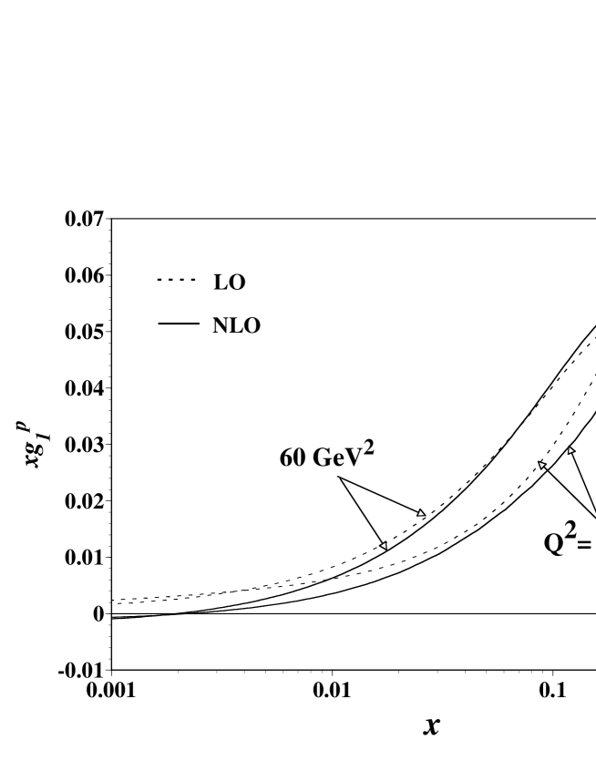
FIG. 1.: $Q^{2}$ evolution results for the proton structure function $g_{1}^{\,p}$. The initial LO and NLO-1 $g_{1}$ structure functions are evolved to those at 60 GeV² by the LO and NLO DGLAP evolution equations.

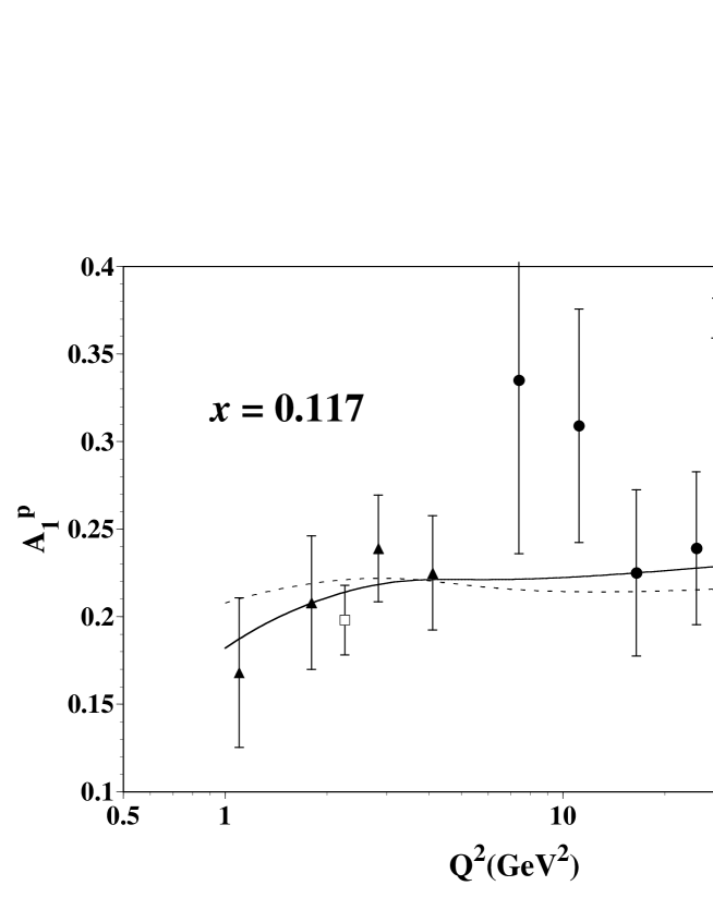
FIG. 2.: Calculated LO and NLO spin asymmetries $A_{1}$ for the proton are compared with the experimental results by the SMC, SLAC-E143, and HERMES collaborations at $x\approx 0.117$. The theoretical curves are obtained by using our LO and NLO-1 fitting results at $Q^{2}$=1 GeV².

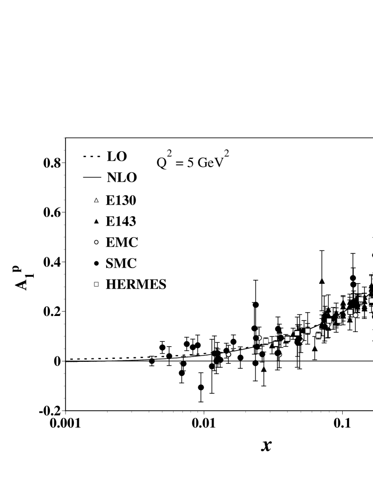
(a)

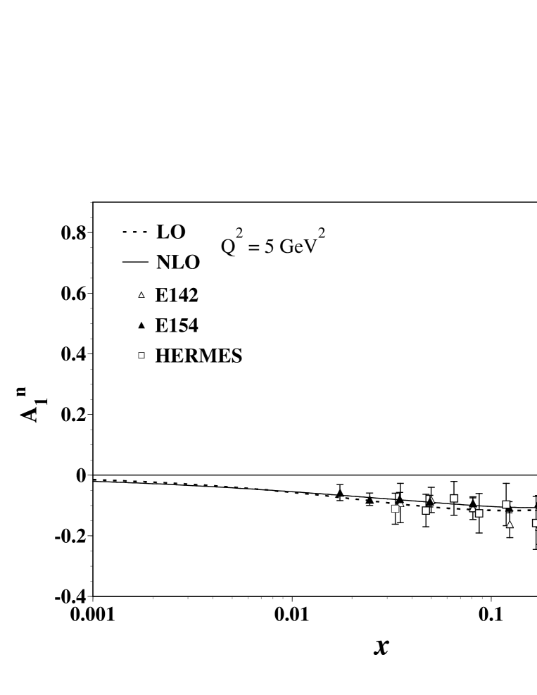
(b)

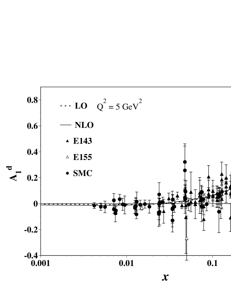
(c)

FIG. 3.: Comparison of our calculations with the experimental asymmetry $A_{1}(x,Q^{2})$ data for the (a) proton, (b) neutron, and (c) deuteron. Our results are obtained at $Q^{2}$=5 GeV² with the optimum parameters in Tables II (LO) and III (NLO-1). The NLO and LO results are shown by the solid and dotted lines, respectively.

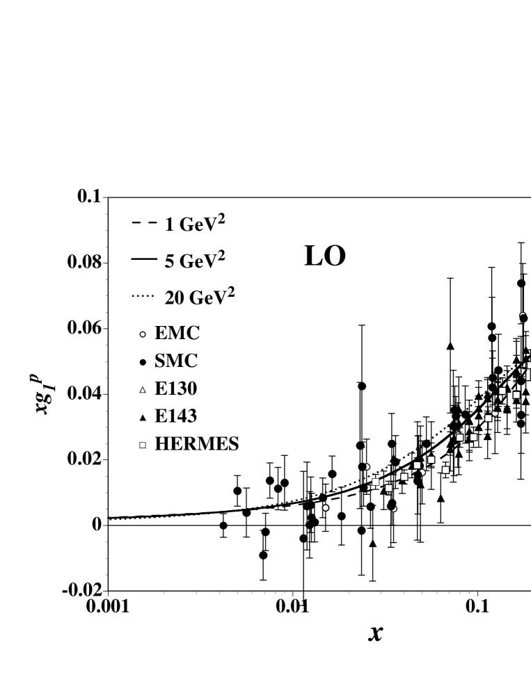
(a)

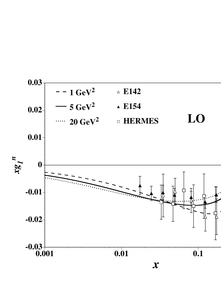
(b)

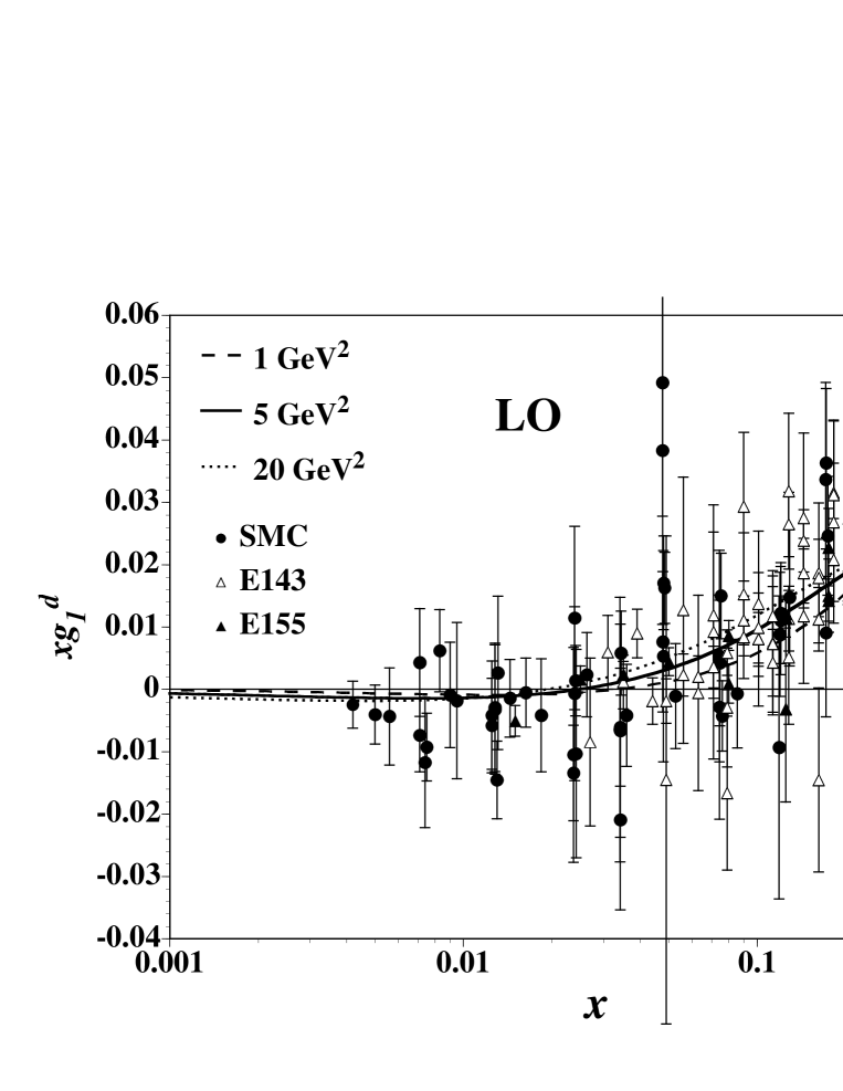
(c)

FIG. 4.: Experimental spin-dependent structure functions $xg_{1}(x,Q^{2})$ are compared with our LO results for the (a) proton, (b) neutron, and (c) deuteron. Our fitting results are calculated at $Q^{2}$=1, 5, 20 GeV² by using the LO evolution equations with the optimum parameters in Table II, and they are shown by the dashed, solid, and dotted curves, respectively. The experimental data are obtained from the $A_{1}(x,Q^{2})$ data and the $F_{2}(x,Q^{2})$ calculated with the unpolarized GRV distributions and $R_{1990}(x,Q^{2})$.

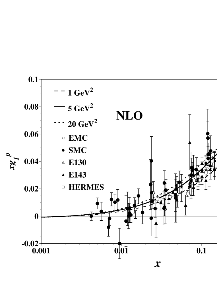
(a)

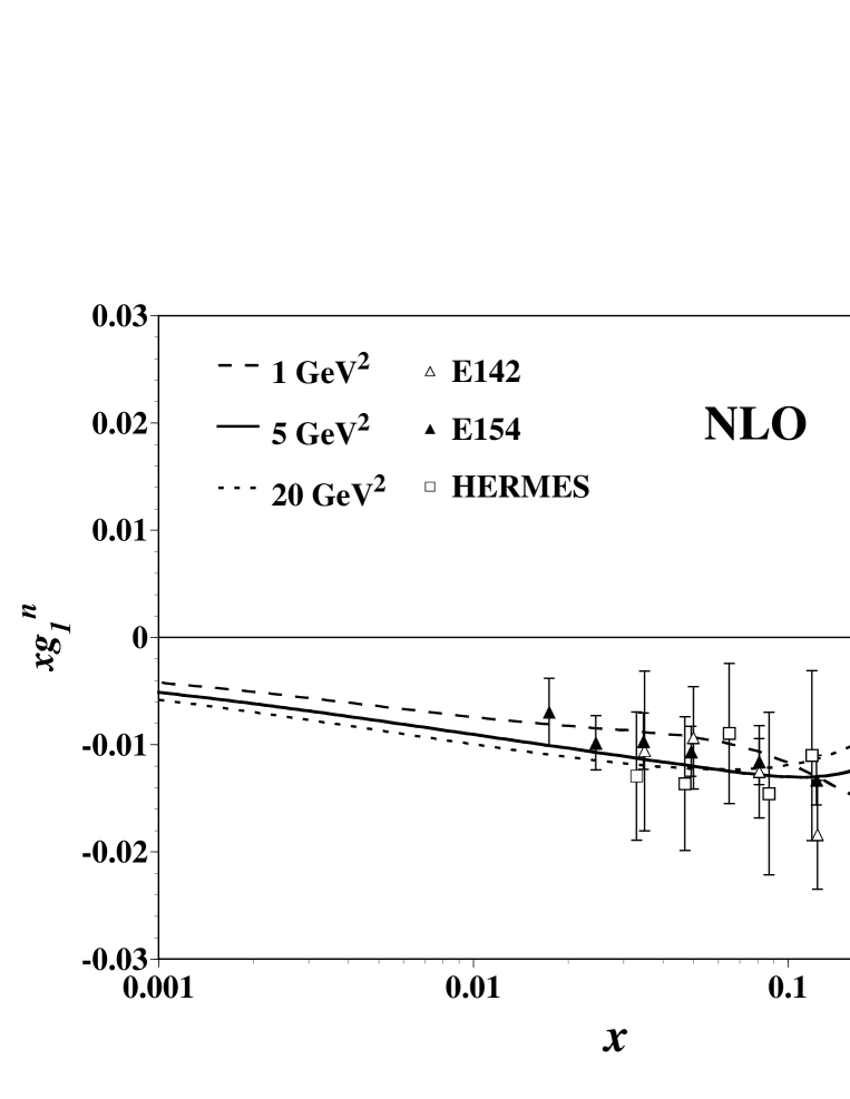
(b)

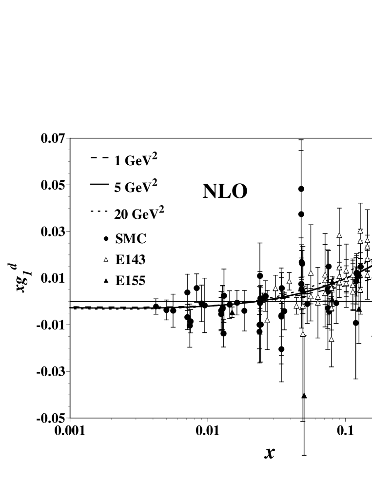
(c)

FIG. 5.: Experimental data of $xg_{1}(x,Q^{2})$ are compared with our NLO-1 results for the (a) proton, (b) neutron, and (c) deuteron. The notations are the same as those in Fig. 4.

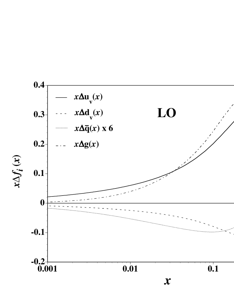
(a)

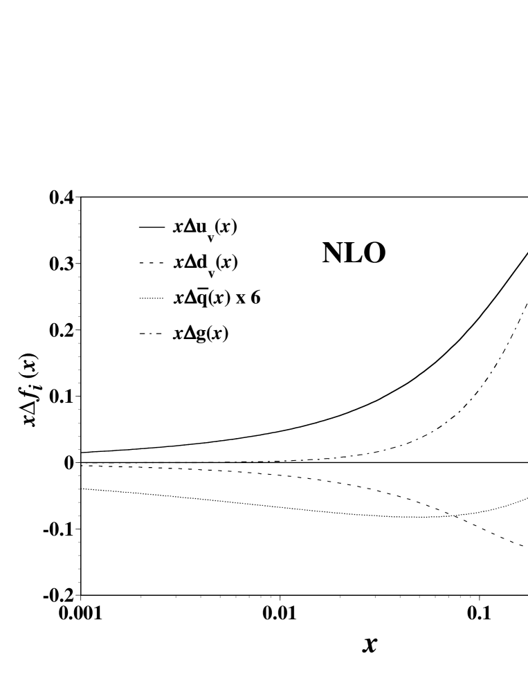
(b)

FIG. 6.: Obtained LO and NLO-1 polarized parton distributions $x\Delta f_{i}(x,Q^{2})$ at $Q^{2}=1$ GeV² in (a) and (b), respectively.

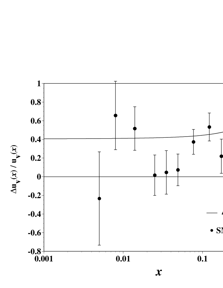
(a)

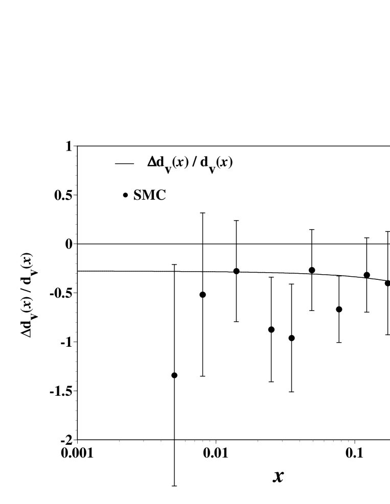
(b)

FIG. 7.: Our LO ratios $\Delta u_{v}/u_{v}$ and $\Delta d_{v}/d_{v}$ are compared with the SMC data in (a) and (b), respectively. Our results are calculated at $Q^{2}=10$ GeV² by using the polarized distributions in the LO.

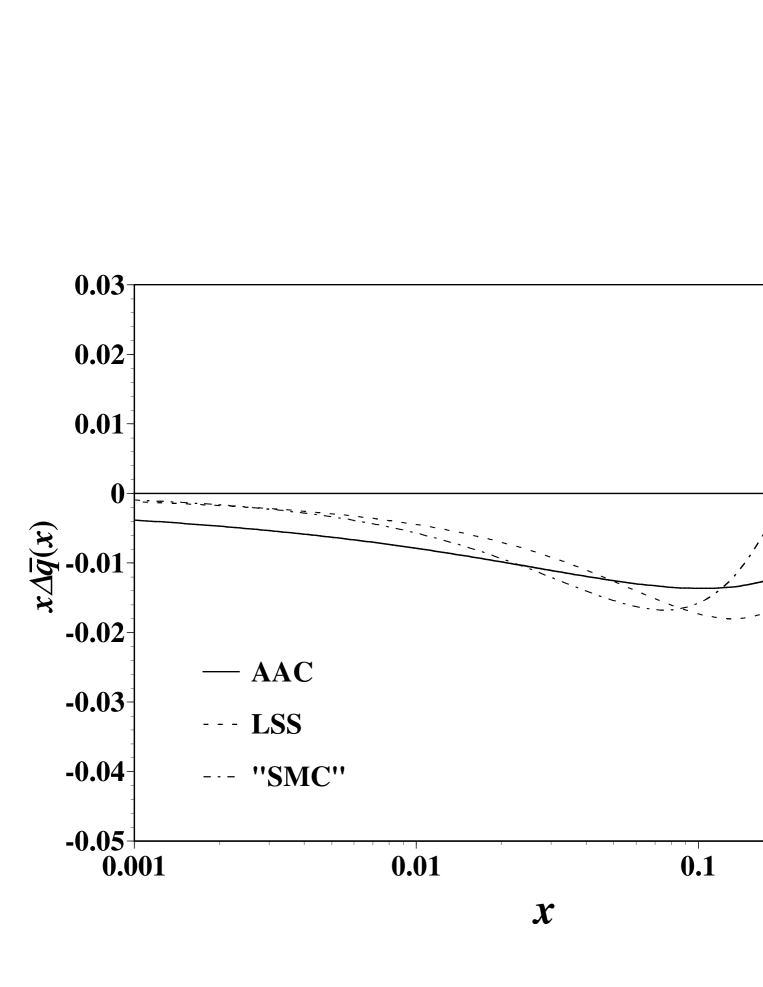
FIG. 8.: The antiquark distributions of transformed SMC (“SMC”) and LSS(1999) are compared with our NLO-1 distribution at $Q^{2}$=1 GeV².

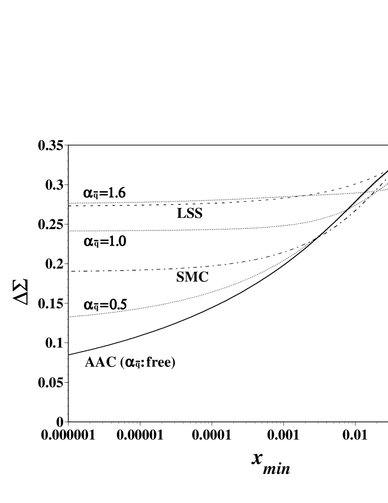
FIG. 9.: The $x_{min}$ dependence of $\Delta\Sigma(x_{min})=\int_{x_{min}}^{1}\Delta\Sigma(x)dx$ is compared with the recent parametrizations of SMC and LSS(1999) at $Q^{2}$=1 GeV².

REFERENCES

- [1] European Muon Collaboration (EMC), J. Ashman et al., Phys. Lett. B206, 364 (1988); Nucl. Phys. B328, 1 (1989).
- [2] Spin Muon Collaboration (SMC), B. Adeva et al., Phys. Rev. D58, 112001 (1998).
- [3] SMC, B. Adeva et al., Phys. Lett. B412, 414 (1997).
- [4] SLAC-E143 collaboration, K. Abe et al., Phys. Rev. D58, 112003 (1998).
- [5] HERMES collaboration, K. Ackerstaff et al., Phys. Lett. B404, 383 (1997); A. Airapetian et al., Phys. Lett. B442, 484 (1998).
- [6] G. Bunce et al., Particle World 3, 1 (1992).
- [7] Common Muon and Proton Apparatus for Structure and Spectroscopy (COMPASS) collaboration, G. Baum et al., CERN/SPSLC 96-14 (unpublished).
- [8] R. Mertig and W. L. van Neerven, Z. Phys. C70, 637 (1996).
- [9] W. Vogelsang, Phys. Rev. D54, 2023 (1996).
- [10] M. Glück, E. Reya, M. Stratmann, and W. Vogelsang, Phys. Rev. D53, 4775 (1996).
- [11] T. Gehrmann and W. J. Stirling, Phys. Rev. D53, 6100 (1996).
- [12] G. Altarelli, R. D. Ball, S. Forte, and G. Ridolfi, Nucl. Phys. B496, 337 (1997); Acta Phys. Pol. B29, 1145 (1998).
- [13] C. Bourrely, F. Buccella, O. Pisanti, P. Santorelli, and J. Soffer, Prog. Theor. Phys. 99, 1017 (1998).
- [14] L. E. Gordon, M. Goshtasbpour, and G. P. Ramsey, Phys. Rev. D58, 094017 (1998); G. P. Ramsey, Prog. Part. Nucl. Phys. 39, 599 (1997).
- [15] SMC, B. Adeva et al., Phys. Rev. D58, 112002 (1998).
- [16] E. Leader, A. V. Sidrov, and D. B. Stamenov, Phys. Rev. D58, 114028 (1998); Phys. Lett. B445, 232 (1998); B462, 189 (1999).
- [17] J. A. Gracey, J. Phys. G25, 1547 (1999).
- [18] L. W. Whitlow, S. Rock, A. Bodek, S. Dasu, and E. M. Riordan, Phys. Lett. B250, 193 (1990); L. W. Whitlow, report SLAC-0357 (1990).
- [19] New Muon Collaboration (NMC), M. Arneodo et al., Nucl. Phys. B483, 3 (1997).
- [20] S. Kumano, Phys. Rep. 303, 183 (1998); J.-C. Peng and G. T. Garvey, hep-ph/9912370.
- [21] T. Morii and T. Yamanishi, hep-ph/9905294, to be published in Phys. Rev. D.
- [22] N. Saito, in Spin structure of the nucleon, edited by T.-A. Shibata, S. Ohta, and N. Saito, (World Scientific, Singapare, 1996).
- [23] S. Kumano and M. Miyama, hep-ph/9909432, Phys. Lett. B in press.
- [24] R. D. Ball, S. Forte, and G. Ridolfi, Phys. Lett. B378, 255 (1996).
- [25] S. L. Adler and W. A. Bardeen, Phys. Rev. 182, 1517 (1969).
- [26] M. Anselmino, A. Efremov, and E. Leader, Phys. Rep. 261, 1 (1995).
- [27] H.-Y. Cheng, Int. J. Mod. Phys. A11, 5109 (1996).
- [28] J. F. Gunion, Phys. Rev. D10, 242 (1974); R. Blankenbeckler and S. J. Brodsky, Phys. Rev. D10, 2973 (1974); G. R. Farrar and D. R. Jackson, Phys. Rev. Lett. 35, 1416 (1975).
- [29] C. Bourrely, E. Leader, O. V. Teryaev, hep-ph/9803238 (unpublished).
- [30] S. J. Brodsky, M. Burkardt, and I. Schmidt, Nucl. Phys. B441, 197 (1995).
- [31] SLAC-E130 collaboration G. Baum et al., Phys. Rev. Lett. 51, 1135 (1983).
- [32] SLAC-E142 collaboration, P. L. Anthony et al., Phys. Rev. D54, 6620 (1996).
- [33] SLAC-E154 collaboration, K. Abe et al., Phys. Rev. Lett. 79, 26 (1997).
- [34] SLAC-E155 collaboration, P. L. Anthony et al., Phys. Lett. B463, 339 (1999).
- [35] M. Glück, E. Reya, and A. Vogt, Eur. Phys. J. C5, 461 (1998).
- [36] A. D. Martin, R. G. Roberts, W. J. Stirling, and R. S. Thorne, Eur. Phys. J. C4, 463 (1998).
- [37] CTEQ collaboration, H. L. Lai et al., hep-ph/9903282, to be published in Eur. Phys. J. C (1999).
- [38] M. Miyama and S. Kumano, Comput. Phys. Commun. 94, 185 (1996); M. Hirai, S. Kumano, and M. Miyama, loc. cit. 108, 38 (1998).
- [39] Particle Data Group, Eur. Phys. J. C3, 1 (1998).
- [40] F. James, CERN Program Library Long Writeup D506 (unpublished).
- [41] SMC, B. Adeva et al., Phys. Lett. B420, 180 (1998).
- [42] For example, see http://quark.phy.bnl.gov/~raju/eRHIC.html.
- [43] J. Ellis and M. Karliner, Phys. Lett. B213, 73 (1988).
- [44] B. Lampe and E. Reya, hep-ph/9810270.
- [45] F. E. Close and R. G. Roberts, Phys. Rev. Lett. 60, 1471 (1988).
- [46] N. Saito, Nucl. Phys. B (Proc. Suppl.) 79, 584 (1999).