Non-leptonic hyperon weak decays in the Skyrme model revisited

Abstract

Non-leptonic hyperon weak decays are investigated in the $SU(3)$ Skyrme model. We use a collective coordinate scheme, following the approach in which the symmetry breaking terms in the strong effective action are diagonalized exactly. To describe the weak interactions we use an octet dominated weak effective lagrangian that leads to a good description of the known $2\pi$ and $3\pi$ kaon decays. We show that the observed $S$-wave decays are reasonably well reproduced in the model. On the other hand, our calculated $P$-wave amplitudes do not agree with the empirical ones even though both pole and contact contributions to these amplitudes are properly taken into account. Finally, an estimate of the non-octet contributions to the decay amplitudes is presented.

I Introduction

Although during the last few decades much progress has been done in the theoretical study of hadron structure, the non-leptonic weak decays of hyperons still remain far from being well understood. This class of decays involve not only weak interactions but also low momentum strong processes, which have made their first principle calculation unfeasible so far. In this situation, different hadron models have been used to get the corresponding theoretical predictions. The available experimental information allows to determine both $S$- and $P$-wave decay amplitudes separately for various processes. In the case of the $S$-wave decays, the predictions given by quark models with QCD enhancement factors turn out to be quite successful (see Ref.[1] and references therein). These models, however, have serious difficulties in reproducing at the same time the empirical results in the case of the $P$-wave amplitudes. Indeed, this seems to be a problem (so called “$S/P$ wave puzzle”) which is common to other approaches as e.g. heavy baryon chiral perturbation theory[2], QCD sum rules[3], etc.

A possible solution to the $S/P$ wave puzzle has been suggested some years ago within the context of chiral topological soliton models[1, 4]. It was shown that in these models the $P$-wave amplitudes receive, in addition to the standard pole diagrams, extra contributions from contact terms. Then, it was speculated that these extra terms could provide a clue to this issue. Unfortunately, at the time this suggestion was made such models were hampered by several serious problems, such as very poor predictions for the hyperon spectrum[5], far too small results for the $S$-wave non-leptonic decay amplitudes[4, 6], etc. Therefore, it was hard to draw definite conclusions about the real relevance of the contact terms. With the introduction of more refined methods to treat the chiral symmetry breaking terms in the effective action the situation has significantly improved. Indeed, a scheme in which one introduces $SU(3)$ collective coordinates and the hamiltonian —including a symmetry breaking piece— is diagonalized exactly leads to very good results for the hyperon spectra, as well as reasonable predictions for different baryon properties (for a review see Ref.[7]). Moreover, it has been recently shown[8] that within such scheme, and using a simple Cabbibo current-current form for the weak interaction, one can obtain the correct $S$-wave absolute values. Thus, we are now in position to verify whether chiral soliton models can provide a unified and consistent description of the hyperon non-leptonic decays. In this work we will describe the weak interactions by means of an effective weak chiral lagrangian —which is more general than the Cabbibo current-current coupling often used in previous Skyrme model calculations [6, 8, 9, 10]—, where the low energy coupling constants will be fixed to reproduce the known $2\pi$ and $3\pi$ $K$-meson decays. We will concentrate mostly in the dominant octet-like piece of this $\Delta S=1$ lagrangian, considering terms up to order $p^{4}$. In addition, possible non-octet contributions will be considered for the particular case of the ${\cal A}(\Sigma^{+}_{+})$ amplitude which, as well known, vanishes in the pure octet approximation. The non-leptonic hyperon decay amplitudes will be obtained by evaluating the corresponding matrix elements using the topological soliton model wave functions.

The article is organized as follows: in Sec. II we give a brief overview of the $SU(3)$ soliton model and introduce the octet-like weak effective chiral lagrangian to be used in the following two sections. In Sec. III and IV we describe the calculation of the $S$-wave and $P$-wave amplitudes respectively, and present the corresponding results. The impact of the non-octet-like components of the weak effective lagrangian is discussed in Sec. V and in Sec. VI we state our conclusions. Finally, in the Appendix we give some details concerning the evaluation of the matrix elements of the collective operators which appear in the calculation of the decay amplitudes.

II The model

In chiral topological soliton models baryons are described as topological excitations of a chiral effective action which depends only on meson fields. We use the form

$$\Gamma=\Gamma_{SK}+\Gamma_{WZ}+\Gamma_{SB}\ ,$$ (1)

where $\Gamma_{SK}$ and $\Gamma_{WZ}$ stand for the Skyrme and Wess-Zumino actions respectively, and $\Gamma_{SB}$ is an $SU(3)$ symmetry breaking piece. The Skyrme action has the usual form

$$\Gamma_{SK}=\int d^{4}x\Big{\{}{f^{2}_{\pi}\over 4}{\,\mbox{Tr}}\left[\partial_{\mu}U(\partial^{\mu}U)^{\dagger}\right]+{1\over{32\epsilon^{2}}}{\,\mbox{Tr}}\left[[U^{\dagger}\partial_{\mu}U,U^{\dagger}\partial_{\nu}U]^{2}\right]\Big{\}}\,,$$ (2)

where the chiral field $U$ is a non–linear realization of the pseudoscalar octet, $f_{\pi}=93$ MeV is the pion decay constant and $\epsilon$ is the dimensionless Skyrme parameter. The Wess-Zumino action reads

$$\Gamma_{WZ} = -{iN_{c}\over{240\pi^{2}}}\int d^{5}x\,\epsilon^{\mu\nu\rho\sigma\tau}{\,\mbox{Tr}}\,[L_{\mu}L_{\nu}L_{\rho}L_{\sigma}L_{\tau}]\,,$$ (3)

where $L_{\mu}=U^{\dagger}\partial_{\mu}U$ and $N_{c}=3$ is the number of colors. Finally the symmetry breaking piece $\Gamma_{SB}$ is given by

$$\Gamma_{SB} = \int d^{4}x\left\{{f_{\pi}^{2}m_{\pi}^{2}+2f_{K}^{2}m_{K}^{2}\over{12}}{\,\mbox{Tr}}\left[U+U^{\dagger}-2\right]+\sqrt{3}{f_{\pi}^{2}m_{\pi}^{2}-f_{K}^{2}m_{K}^{2}\over{6}}{\,\mbox{Tr}}\left[\lambda_{8}\left(U+U^{\dagger}\right)\right]\right.$$ (5)

$$\qquad\left.+{f_{K}^{2}-f_{\pi}^{2}\over{12}}{\,\mbox{Tr}}\left[(1-\sqrt{3}\lambda_{8})\left(U(\partial_{\mu}U)^{\dagger}\partial^{\mu}U+U^{\dagger}\partial_{\mu}U(\partial^{\mu}U)^{\dagger}\right)\right]\right\}\,,$$

where $f_{K}$ is the kaon decay constant and $m_{\pi}$ and $m_{K}$ are the pion and kaon masses, respectively. In our numerical calculations below we will set these parameters to their empirical values and take $\epsilon=4.1$ which is suitable for a good description of many baryon properties in this model.

In the soliton picture we are using the strong interaction properties of the low–lying $\frac{1}{2}^{+}$ and $\frac{3}{2}^{+}$ baryons are computed following the standard $SU(3)$ collective coordinate approach to the Skyrme model. We introduce for the chiral field the ansatz

$$U_{0}({\bf r},t)=A(t)\ \left(\begin{array}[]{cc}c\ \openone+i\mbox{\boldmath$\tau$}\cdot{\hat{\mbox{\boldmath$r$}}}\ s&0\\ 0&1\end{array}\right)\ A^{\dagger}(t)\ ,$$ (6)

where we have used the abbreviations $c=\cos F(r)$ and $s=\sin F(r)$, $F(r)$ being the chiral angle that parameterizes the soliton. The collective rotation matrix $A(t)$ is $SU(3)$ valued. Substituting the configuration Eq. (6) into $\Gamma$ yields (upon canonical quantization of $A$) the collective Hamiltonian. Its eigenfunctions are identified as the baryon wavefunctions $\Psi_{B}$. Due to the symmetry breaking piece $\Gamma_{SB}$, the Hamiltonian is obviously not $SU(3)$ symmetric. However, as shown by Yabu and Ando [11], it can be diagonalized exactly. The diagonalization essentially amounts to admixtures of states from higher $SU(3)$ representations into the octet ($J=\frac{1}{2}$) and decouplet ($J=\frac{3}{2}$) states. This procedure has proven to be quite successful in describing the hyperon spectrum and static properties [7].

In order to describe the non-leptonic hyperon decays we have to introduce an effective weak $\Delta S=1$ lagrangian. The latter is constrained by weak interactions to transform either as $\underline{8}$ or $\underline{27}$ under the chiral group $SU(3)_{L}$. Here, we will take into account only the dominant octet-like couplings, which lead to pure $\Delta I=1/2$ transitions. The remaining $\underline{27}$ piece includes both $\Delta I=1/2$ and $\Delta I=3/2$ operators and turns out to be suppressed in view of the yet not completely understood “$\Delta I=1/2$ rule”. Further considerations about these non-octet-like terms will be given in Sec. V. We consider the effective lagrangian given by [14]

$${\cal L}^{(8)}_{w}=g{\,\mbox{Tr}}\,[\lambda_{6}\partial_{\mu}U\partial^{\mu}U^{\dagger}]+g^{\prime}{\,\mbox{Tr}}\,[\lambda_{6}\partial_{\mu}U\partial^{\mu}U^{\dagger}\partial_{\nu}U\partial^{\nu}U^{\dagger}]+g^{\prime\prime}{\,\mbox{Tr}}\,[\lambda_{6}\partial_{\mu}U\partial_{\nu}U^{\dagger}\partial^{\mu}U\partial^{\nu}U^{\dagger}]\ .$$ (7)

It should be noticed that this is not the most general octet-like $\Delta S=1$ interaction one can write down up to ${\cal O}(p^{4})$ in the momentum power expansion. The latter, containing many other terms, has been presented in Ref.[12]. For the decays we are interested in (no external fields), it turns out that the most general lagrangian includes 15 independent terms of order $p^{4}$ leading to pure $\Delta I=1/2$ transitions. However, to this order, it has been shown[13] that the couplings considered in (7) are sufficient to fit the known data on $K\to\pi\pi$ and $K\to\pi\pi\pi$. In the absence of further information from the meson sector, we will just stick to this simple form. In order to give an idea of the uncertainties in our calculations, we will consider two sets of values for the constants $g,g^{\prime}$ and $g^{\prime\prime}$ which provide fits to the kaon data of similar quality. Set A corresponds to the parameters used in Refs. [4, 14],

$$g=3.60\times 10^{-8}\ m_{\pi}^{2}\quad;\quad g^{\prime}/g=1.50\times 10^{-1}\ {\rm fm}^{2}\quad;\quad g^{\prime\prime}/g=-6.74\times 10^{-2}\ {\rm fm}^{2}\;,$$ (8)

while Set B corresponds to the values obtained in Ref.[13],

$$g=2.98\times 10^{-8}\ m_{\pi}^{2}\quad;\quad g^{\prime}/g=1.69\times 10^{-1}\ {\rm fm}^{2}\quad;\quad g^{\prime\prime}/g=1.87\times 10^{-2}\ {\rm fm}^{2}\;.$$ (9)

To calculate the hyperon decays in the context of the Skyrme model with $SU(3)$ collective coordinates, we include the soft meson fluctuations on top of the soliton background. This is achieved using

$$U=U_{M}\ U_{0}({\bf r},t)\ U_{M}\ ,$$ (10)

where $U_{M}=1+i\vec{\tau}\cdot\vec{\pi}/(2\,f_{\pi})+...$. Inserting this expression into ${\cal L}^{(8)}_{w}$ and taking the appropriate matrix elements one can obtain the desired $S$-wave and $P$-wave decay amplitudes. This is worked out in the following two sections.

III $S$-wave amplitudes

As mentioned in the Introduction, it has been recently shown[8] that if the Cabbibo current-current form is used to describe the weak interactions, the present soliton model leads to a reasonably good description of the $S$-wave hyperon decay amplitudes. In this section we study these amplitudes using the effective weak chiral lagrangian given by Eqs. (7–9).

As usual, we assume that isospin symmetry is preserved. In such limit, the following relations between the non-leptonic decay amplitudes can be derived:

$$\Sigma^{-}_{-} = \Sigma_{+}^{+}-\sqrt{2}\ \Sigma^{+}_{0}$$ (12)

$$\Lambda_{-}^{0} = -\sqrt{2}\ \Lambda^{0}_{0}$$ (13)

$$\Xi_{-}^{-} = -\sqrt{2}\ \Xi^{0}_{0}\ ,$$ (14)

where the lower indices indicate the charge of the outgoing pion. In this way, only four of the seven measurable amplitudes need to be considered as independent. For simplicity, we choose these amplitudes to be $\Lambda^{0}_{0}$, $\Sigma^{+}_{0}$, $\Xi^{0}_{0}$ and $\Sigma_{+}^{+}$.

For a process $B\rightarrow B^{\prime}\pi$, we can define the amplitudes ${\cal A}$ and ${\cal B}$, corresponding to $S$- and $P$-wave decays respectively, according to

$$i\,\langle B^{\prime}\pi|{\cal L}^{(8)}_{w}|B\rangle=\bar{u}_{B^{\prime}}\,({\cal A}+{\cal B}\,\gamma_{5})\,u_{B}\ .$$ (15)

In the soft-pion limit, the octet nature of ${\cal L}^{(8)}_{w}$, together with current algebra relations, lead to an additional constraint for the $S$-wave $\Sigma$ decay amplitudes, namely ${\cal A}(\Sigma^{-}_{-})=-\sqrt{2}\,{\cal A}(\Sigma^{+}_{0})$. Thus from (12) one obtains ${\cal A}(\Sigma^{+}_{+})=0$. The remaining ${\cal A}$ amplitudes can be calculated by replacing Eqs. (10) and (6) in ${\cal L}^{(8)}_{w}$ and taking the corresponding matrix elements. We find

$${\cal A}(B\rightarrow B^{\prime}\pi^{0})=\alpha\ \langle B^{\prime}|R_{78}|B\rangle\,,$$ (16)

where

$$\alpha=\frac{4\pi\,i}{\sqrt{3}f_{\pi}}\int dr\ r^{2}\left[g\left(F^{\prime 2}+2\ \frac{\sin^{2}F}{r^{2}}\right)-g^{\prime}\left(F^{\prime 2}+2\ \frac{\sin^{2}F}{r^{2}}\right)^{2}-g^{\prime\prime}\left(F^{\prime 4}-4\ \frac{F^{\prime 2}\sin^{2}F}{r^{2}}\right)\right]\,.$$ (17)

In Eq. (16), $R_{78}$ stands for an $SU(3)$ rotation matrix, $R_{ab}=1/2\ {\,\mbox{Tr}}\left[\lambda_{a}A\lambda_{b}A^{\dagger}\right]$. As explained in the Appendix, its matrix elements between the collective wavefunctions describing the different baryon states can be calculated as linear combinations of $SU(3)$ Clebsch-Gordan coefficients.

Our results for the ${\cal A}$ amplitudes are summarized in Table I, where we also quote the values corresponding to the quark model (QM) [1]. Following the usual convention, the overall phase has been fixed to obtain ${\cal A}(\Lambda^{0}_{-})$ real and positive. It can be seen from the table that the predictions obtained with Set A are about 15 % higher than those arising from Set B. In both cases, our results are somewhat below the experimental values. However, since the deviation is in the same direction for all processes (notice that this is not the case for the QM values), the agreement is significantly improved if one considers the ratios between the different amplitudes. In general, it could be said that our results and those corresponding to the QM are of similar quality.

It is also interesting to compare the present results with those of previous soliton calculations. As already mentioned, in some of them[6, 8, 9, 10] the Cabbibo current-current has been used. Within such scheme the best agreement with empirical data has been obtained in Ref.[8] where, as done here, the baryon wavefunctions arise from an exact diagonalization of the SU(3) collective hamiltonian. Generally speaking the results reported in Table I are somewhat smaller (in absolute value) than those of Ref.[8]. However, it should be stressed that the present calculation is free from the uncertainties related to the question of whether (and to which extent) QCD enhancement factors have to be included in soliton calculations. Here, such factors are already accounted for in the value of the low energy constants that appear in the weak lagrangian. On the other hand, if our results are compared with previous calculations based on effective weak chiral lagrangians[4], we see that the use of empirical input parameters in the strong effective action, together with the exact diagonalization of the SU(3) collective hamiltonian, lead to a significant improvement in the predictions.

A final comment concerns Ref.[16] and its Addendum [17]. In Ref.[16], the author studies weak decays of hyperons in a chiral topological soliton model, starting with a $\Delta S=1$ lagrangian including six ${\cal O}(p^{4})$ terms. As shown in the Addendum, the Cayley-Hamilton theorem can be used to reduce these six terms to only four independent ones. Moreover, following the same steps as in our calculation, one arrives to further relations between the corresponding hyperon decay amplitudes. At the end one is effectively left with only two terms, which —as done in the present work— can be chosen to be those proportional to $g^{\prime}$ and $g^{\prime\prime}$ in Eq. (7). Following Ref.[16], one might try to see whether it is possible to find a set of coefficients for those terms capable to reproduce the empirical values for both kaon and hyperon decays. For this purpose, and in order to relate the coefficients with the hyperon amplitudes, the author of Ref.[16] makes use of the relation (16) and takes the $SU(3)$ symmetric limit. In this way all decay amplitudes can be expressed in terms of one of them and the $f/d$ ratio. The use of empirical values for the latter leads to an incompatible system of equations, so that the author argues that this precludes a successful application of the chiral lagrangian model. We believe that the results found in the present work provide some ground to disagree with such strong conclusion. In fact, the relations in Ref.[16] are expected to be modified by $SU(3)$ breaking effects and by next-to-leading order corrections in $N_{c}$, which in general introduce modifications to Eq. (16). From the results displayed in Table I it is seen that if the chiral soliton approach is used together with an effective weak chiral lagrangian consistent with $K$ meson decays, one can obtain a reasonably good description of the $S$-wave hyperon decays, already at leading order in $N_{c}$.

IV $P$-wave amplitudes

We turn now to the evaluation of the $P$-wave amplitudes. In the non-relativistic limit, they can be calculated using

$${\cal B}\,\bar{u}_{B^{\prime}}\,\gamma_{5}\,u_{B}\simeq-{{\cal B}\over{2\overline{M}}}\ \chi^{\dagger}(\lambda^{\prime})\ \vec{\sigma}\cdot\vec{q}\ \chi(\lambda)\ ,$$ (18)

where $\overline{M}$ is the average of the $B$ and $B^{\prime}$ empirical masses. As stated in the Introduction, in the present model ${\cal B}$ receives contributions of two different kinds[4]. One of them arises from contact terms in ${\cal L}^{(8)}_{w}$ (see Fig. 1a), whereas the other one is given by the pole diagrams shown in Figs. 1b-1d. Our evaluation of the contact contribution in the case of $\pi^{0}$ emission leads to

$${\cal B}_{contact}(B\rightarrow B^{\prime}\pi^{0})=-\frac{2\overline{M}}{3f_{\pi}}\ \langle B^{\prime}|\int d^{3}r\ {\hat{\cal P}}_{c}|B\rangle\,,$$ (19)

where

$${\hat{\cal P}}_{c} = \quad g\left\{(1+c)(F^{\prime}+2\frac{s}{r})R_{63}-\frac{2}{\sqrt{3}}(1-c)(F^{\prime}-2\frac{s}{r})R_{3}^{(+)}\right\}$$ (24)

$$+\;g^{\prime}\left(F^{\prime 2}+2\frac{s^{2}}{r^{2}}\right)\left\{-(1+c)(F^{\prime}+2\frac{s}{r})R_{63}+\frac{2}{\sqrt{3}}\left[F^{\prime}(3-c)+2\frac{s}{r}(3c-1)\right]R_{3}^{(+)}\right\}$$

$$+\;g^{\prime\prime}\left\{(1+c)F^{\prime}\left(-F^{\prime 2}+2\frac{s}{r}F^{\prime}+2\frac{s^{2}}{r^{2}}\right)R_{63}\right.$$

$$\qquad\qquad\left.+\frac{2}{\sqrt{3}}\left[F^{\prime 3}(3-c)+2\frac{s}{r}F^{\prime}(1-c)(F^{\prime}-\frac{s}{r})+4\frac{s^{3}}{r^{3}}c\right]R_{3}^{(+)}\right.$$

$$\left.\qquad\qquad-\frac{8}{\sqrt{3}}\frac{s}{r}\left[cF^{\prime 2}+F^{\prime}\frac{s}{r}+c\frac{s^{2}}{r^{2}}\right]R_{3}^{(-)}\right\}\;,$$

with

$$R_{3}^{(\pm)}=R_{68}R_{33}\pm R_{63}R_{38}\;.$$ (25)

Similar expressions can be found in the case of charged outgoing pions. On the other hand, from the pole diagrams we obtain

$${\cal B}_{pole}(B\rightarrow B^{\prime}\pi^{0})=-2\sqrt{2}\ \overline{M}\ \sum_{B^{\prime\prime}}\left[g_{A}^{B^{\prime}B^{\prime\prime}}\frac{{\cal A}(B\rightarrow B^{\prime\prime}\pi^{0})}{M_{B}-M_{B^{\prime\prime}}}+g_{A}^{BB^{\prime}}\frac{{\cal A}(B^{\prime\prime}\rightarrow B^{\prime}\pi^{0})}{M_{B^{\prime}}-M_{B^{\prime\prime}}}\right]\ ,$$ (26)

where we have neglected the small $K$ pole term contribution in Fig. 1d, and we have made use of the generalized Goldberger-Treiman relations to write the strong coupling constants in terms of the axial charges. Notice that Eq. (26) includes a sum over a set of intermediate states $B^{\prime\prime}$. In our calculations, we have included the $J^{\pi}=\frac{1}{2}^{+}$ collective eigenfunctions that arise from the exact diagonalization of the strong Hamiltonian. It turns out that only a few excited states are needed to find convergence and their contribution represents, at most, $15\%$ of the total values of ${\cal B}_{pole}$.

For the sake of consistency, in order to estimate the size of the ${\cal B}_{pole}$ amplitudes we will take into account both the axial charges and the ${\cal A}$ amplitudes obtained within our model. Therefore, we consider the axial charge operator $\hat{g}_{A}$ arising from the action (1), which reads

$$\frac{\hat{g}_{A}}{\sqrt{2}} = -\frac{1}{3}\int d^{3}r\left\{f_{\pi}^{2}\left(F^{\prime}+2c\frac{s}{r}\right)+\frac{2}{e^{2}}\frac{s}{r}\left(c\frac{s^{2}}{r^{2}}+\frac{s}{r}F^{\prime}+cF^{\prime 2}\right)\right\}R_{33}$$ (29)

$$+\frac{f_{K}^{2}-f_{\pi}^{2}}{9}\int d^{3}r\ (1-c)\left\{\left[\frac{2s}{r}(1+2c)+F^{\prime}\right](1-R_{88})R_{33}+\left[\frac{2s}{r}-F^{\prime}\right]R_{83}R_{38}\right\}$$

$$+\frac{N_{c}}{36\pi^{2}\Theta_{K}}\int d^{3}r\ (1-c)\frac{s}{r}\left(\frac{s}{r}-2F^{\prime}\right)d_{3kk^{\prime}}R_{3k}J_{k^{\prime}}\ ,$$

where $\Theta_{K}$ is the kaonic moment of inertia. It is worth to mention that this operator leads to a low value for the neutron beta decay form factor, $g_{A}\simeq 0.75$, compared with the experimental result of about 1.25.

Numerical results for both the contact and pole contributions to the ${\cal B}$ amplitudes are given in Table II. It can be seen that the absolute values for the total amplitudes are far too small in comparison with the experimental results. In the case of the pole contributions, this could be explained in part by an underestimation of the axial form factors, as suggested by the low value in the case of the neutron beta decay. In particular, for ${\cal B}(\Lambda^{0}_{0})$, the contribution obtained from Eq. (26) using the empirical values of the ${\cal A}$ amplitudes and axial charges is in very good agreement with the experimental result (see the value corresponding to the chiral fit in Table II). In our calculation, instead, the suppression arising from the somewhat low predictions for the $S$-wave amplitudes, together with the underestimation of the axial form factors, conspire to end up with a reduction factor of about 1/3. In the case of the remaining $P$-wave amplitudes, it is well known that the usage of phenomenological values in (26) does not allow to get a good fit of the experimental values. In this sense, the contact contributions have been suggested as a possible novel ingredient to solve the discrepancy. Our results show, however, that the values for ${\cal B}_{contact}$ amount at most 1/10 of the empirical ${\cal B}$ amplitudes. Thus, even if the effect goes in the right direction, the contact contributions appear to be too small to represent a potential solution for the $S/P$ problem.

To check the dependence of our results on the Skyrme parameter $\epsilon$ we have considered departures from the central value $\epsilon=4.1$. We find that the absolute values of the amplitudes tend to increase as $\epsilon$ increases. The amplitudes which turn out to be the most sensitive to the variation of $\epsilon$ are those corresponding to the $\Lambda\to n\pi^{0}$ process. For $\epsilon=4.5$, which already implies an increase of more that $25\%$ for the $\Delta N$ splitting, we find, for Set A, ${\cal A}(\Lambda^{0}_{0})\approx-2\times 10^{-7}$ which is quite close to the empirical value ${\cal A}(\Lambda^{0}_{0})_{emp}=-2.37\times 10^{-7}$. However, even in this case, the predicted ${\cal B}(\Lambda^{0}_{0})$ is still more than a factor 2 below the corresponding empirical value. Thus, we can conclude that the statements above are quite robust under variations of the only adjustable parameter in our calculation.

V Contributions of non-octet-like components

As stated in Sec. II, the non-leptonic decay amplitudes are dominated by the octet-like components of the weak effective lagrangian, hence only these components have been considered in the previous two sections. On the other hand, we have also mentioned that this approximation leads to a vanishing $\Sigma_{+}^{+}$ $S$-wave amplitude. In fact, the experimental value of ${\cal A}(\Sigma_{+}^{+})$, although significantly smaller than the other measured $S$-wave amplitudes, is found to be different from zero. In this section we will investigate whether within the present model the standard non-octet-like contributions to the weak effective lagrangian are able to account for this difference. It is clear that such contributions will also modify the results obtained in the previous sections for the other $S$-wave and $P$-wave decay amplitudes. However, the modifications are, in the worst case, of the same order of magnitude than the uncertainties involved in the parameters $g$, $g^{\prime}$ and $g^{\prime\prime}$ in the weak effective lagrangian. Therefore, in what follows we will concentrate only on the $S$-wave $\Sigma_{+}^{+}$ decay amplitude.

The lowest order 27-plet contribution to the weak effective lagrangian occurs at $p^{2}$. It can be written as [12]

$${\cal L}^{(27)}_{2}=c_{3}\ t_{cd}^{ab}\ {\,\mbox{Tr}}\left(Q_{a}^{c}\ U^{\dagger}\partial_{\mu}U\right)\ {\,\mbox{Tr}}\left(Q_{d}^{b}\ U^{\dagger}\partial^{\mu}U\right)$$ (30)

where $\left(Q^{c}_{a}\right)_{ij}=\delta_{cj}\delta_{ai}$, and

$$t_{21}^{31} = t_{12}^{13}=t_{13}^{12}=t_{31}^{21}=\frac{3}{2}\ ,$$ (31)

$$t_{12}^{31} = t_{21}^{13}=t_{13}^{21}=t_{31}^{12}=1\ ,$$ (32)

with $t_{cd}^{ab}=0$ otherwise. As in the case of the octet-like piece, we will take into account also the effect of next-to-leading order couplings. We consider the ${\cal O}(p^{4})$ interaction

$${\cal L}^{(27)}_{4} = \quad g_{1}\ t_{cd}^{ab}\ {\,\mbox{Tr}}\left(Q_{a}^{c}\,L_{\mu}\right)\ {\,\mbox{Tr}}\left(Q_{d}^{b}\ L_{\nu}\,L^{\mu}\,L^{\nu}\right)$$ (35)

$$+\,g_{2}\ t_{cd}^{ab}\ {\,\mbox{Tr}}\left(Q_{a}^{c}\ L_{\mu}\right)\ {\,\mbox{Tr}}\left(Q_{d}^{b}\ \{L^{\mu},L^{2}\}\right)$$

$$+\,g_{3}\ t_{cd}^{ab}\ {\,\mbox{Tr}}\left(Q_{a}^{c}\ [L_{\mu},L_{\nu}]\right)\ {\,\mbox{Tr}}\left(Q_{d}^{b}\ [L^{\mu},L^{\nu}]\right)\ .$$

Once again the most general lagrangian allowed by chiral symmetry includes many possible terms[12], and the coupling constants cannot be fully determined from the available information on the kaon sector. The structure chosen in (35) is, however, sufficient to get a good fit of $2\pi$ and $3\pi$ $K$ decays. From such a fit one obtains[13] $g_{1}\simeq 1.0\times 10^{-10}$, $g_{2}\simeq-0.4\times 10^{-10}$, $g_{3}\simeq 0.1\times 10^{-10}$ together with $c_{3}/f_{\pi}^{2}\simeq-0.8\times 10^{-9}$. This set of values is used in the numerical calculation below.

The desired $S$-wave $\Sigma^{+}_{+}$ amplitude can be now easily obtained by inserting the explicit form of the chiral field $U$ in the effective couplings (30) and (35). By doing this we arrive to

$${\cal A}^{(27)}(\Sigma^{+}\rightarrow n\,\pi^{+})=\frac{\sqrt{15}}{8\sqrt{2}}\;\left(I_{2}\,+\,I_{4}\right)\;\langle n|D^{27}_{-{3\over 2},0}|\,\Sigma^{+}\rangle\ .$$ (36)

Here, the left lower index of the SU(3) Wigner function $D$ stands for $(Y,I,I_{3})=(1,3/2,-3/2)$ while the right lower index corresponds to $(0,0,0)$. The radial integrals $I_{2}$ and $I_{4}$ are given by

$$I_{2} = -\frac{16\pi}{3f_{\pi}}\,c_{3}\int dr\ r^{2}\left(F^{\prime 2}+2\ \frac{\sin^{2}F}{r^{2}}\right)$$ (37)

$$I_{4} = -\frac{16\pi}{3f_{\pi}}\int dr\ r^{2}\left[g_{1}\,F^{\prime 2}\left(F^{\prime 2}-4\ \frac{\sin^{2}F}{r^{2}}\right)+2g_{2}\left(F^{\prime 2}+2\ \frac{\sin^{2}F}{r^{2}}\right)^{2}\right.$$ (39)

$$\qquad\qquad\qquad\quad\left.+\,g_{3}\,\frac{8\,\sin^{2}F}{r^{2}}\left(2\,F^{\prime 2}+\frac{\sin^{2}F}{r^{2}}\right)\right]\ .$$

Even if the integrand of $I_{4}$ is suppressed by the coefficients $g_{i}$ (which are one to two orders of magnitude lower that $c_{3}/f_{\pi}^{2}$), it can be seen that the suppression is compensated by the values of the radial integrals, in such a way that at the end $I_{4}$ dominates over $I_{2}$. Evaluating the matrix element in (36), we finally obtain

$${\cal A}(\Sigma^{+}_{+})\simeq 0.01\times 10^{-7}\ ,$$ (40)

to be compared with the empirical value ${\cal A}_{emp}(\Sigma^{+}_{+})=0.13\times 10^{-7}$ given in Table I. We observe that our estimation for ${\cal A}(\Sigma_{+}^{+})$, although non-vanishing, is roughly one order of magnitude smaller than the empirical result. As in the case of the octet-like contributions this statement remains valid for reasonable variations of the Skyrme parameter around its central value $\epsilon=4.1$.

VI Conclusions

In this work we have revisited the problem of the calculation of the non-leptonic hyperon decay amplitudes in the topological soliton models. We have used the approach to the $SU(3)$ Skyrme model in which both the isospin and the strange degrees of freedom are treated as collective rotations around the usual $SU(2)$ hedgehog ansatz and the symmetry breaking terms in the strong action are diagonalized exactly. To describe the weak interactions we have used a chiral effective action, in which low energy constants are adjusted to describe the known $2\pi$ and $3\pi$ weak kaon decays. For the $S$-wave decay amplitudes we have found that, compared with previous calculations based on effective weak chiral lagrangians[4], the use of empirical input parameters in the strong effective action, together with the exact diagonalization of the $SU(3)$ collective hamiltonian, lead to a significant improvement in the predictions. A similar result has been recently obtained using a Cabbibo current-current type weak interaction[8]. Although our predictions are about $30\%$ below the empirical values we consider them as satisfactory in view of the simplicity of the model and the fact that higher order $N_{c}$ corrections of that size are to be expected. On the other hand, our results badly fail to reproduce the empirical $P$-wave amplitudes. In soliton models, such amplitudes receive two types of contributions[4], namely those arising from the usual pole diagrams and those coming from contact terms. The presence of the latter provided some hope that the long standing $S/P$ wave puzzle could find a solution within these models. Our results show that, unfortunately, such contact contributions are far too small to close the gap between the predictions coming from the pole terms alone and the empirical values. Although one cannot exclude some corrections to these results due to higher order effects neglected in this work (such as e.g. the kaon induced components which are known to play a significant role in the determination of the parity violating $\pi N$ coupling constant[19]), it is difficult to believe that they could lead to a solution of this problem. Finally, we have estimated the contribution to the decay amplitudes coming from non-octet terms in the weak effective action. Since these contributions are generally very small we have concentrated only on the $S$-wave $\Sigma_{+}^{+}$ decay amplitude which, as well known, vanishes if only octet terms are considered. Our result, although non-zero, turns out to be roughly one order of magnitude smaller than the empirical value. This clearly indicates that, within the Skyrme model, more refined wave functions and/or effective weak interactions are needed to understand the subtle effects related with the small violations of the $\Delta I=1/2$ rule observed in the non-leptonic hyperon $S$-wave decays.

Calculation of the collective matrix elements

As explained in the main text the calculation of the decay amplitudes involves the matrix elements of some collective operators $\hat{\cal O}$ between baryon wavefunctions. To evaluate these matrix elements we proceed as follows.

In general, the wavefunction corresponding to a baryon $B$ can be expanded in terms of $SU(3)$ Wigner functions $D^{R}_{\alpha\beta}$,

$$\Psi_{B}=\sum_{R}C_{B}^{R}\,\sqrt{\mbox{dim\,}(R)}\,D_{\alpha\beta}^{R}\;,$$ (41)

where $\alpha=(Y,I,I_{3})$ and $\beta=(1,J,J_{3})$ carry the baryon quantum numbers, and $R$ is the corresponding representation. The coefficients $C_{B}^{R}$ are obtained from the diagonalization procedure described in Sec. II. In addition, the collective operators $\hat{\cal O}$ can always be expressed as

$$\hat{\cal O}=\sum_{\hat{\alpha},\hat{\beta},\hat{R}}\gamma_{\hat{\alpha},\hat{\beta}}^{\hat{R}}\;\;D_{\hat{\alpha},\hat{\beta}}^{\hat{R}}\;,$$ (42)

where $\gamma_{\hat{\alpha},\hat{\beta}}^{\hat{R}}$ are numerical coefficients. These coefficients result from expressing the “cartesian” $SU(3)$ indexes $a=1...8$ in terms of the “spherical” $SU(3)$ indexes $(Y,I,I_{3})$ and performing suitable Clebsch-Gordan series expansions when needed. For example, for the operator $R_{78}$ appearing in Eq. (16) we have

$$R_{78}=\frac{i}{\sqrt{2}}\left[D^{8}_{(1,\frac{1}{2},-\frac{1}{2}),(0,0,0)}-D^{8}_{(-1,\frac{1}{2},\frac{1}{2}),(0,0,0)}\right]\;,$$ (43)

while the combination $R_{3}^{(+)}$ in Eq. (25) can be written as

$$R^{(+)}_{3} = \frac{\sqrt{6}}{10}\left[D^{8}_{(1,\frac{1}{2},-\frac{1}{2}),(0,1,0)}+D^{8}_{(-1,\frac{1}{2},\frac{1}{2}),(0,1,0)}\right]+\frac{1}{10}\left[D^{27}_{(1,\frac{1}{2},-\frac{1}{2}),(0,1,0)}+D^{27}_{(-1,\frac{1}{2},\frac{1}{2}),(0,1,0)}\right]$$ (45)

$$\qquad\qquad-\frac{1}{\sqrt{5}}\left[D^{27}_{(1,\frac{3}{2},-\frac{1}{2}),(0,1,0)}+D^{27}_{(-1,\frac{3}{2},\frac{1}{2}),(0,1,0)}\right]$$

Thus, the matrix element $\langle B^{\prime}|\hat{\cal O}|B\rangle$ can finally be expressed in terms of the standard $SU(3)$ Clebsch-Gordan coefficients[20]. Namely,

$$\langle B^{\prime}|\hat{\cal O}|B\rangle=\sum_{\hat{\alpha},\hat{\beta},\hat{R}}\gamma_{\hat{\alpha},\hat{\beta}}^{\hat{R}}\;\sum_{R,R^{\prime},\mu}C_{B}^{R}\;(C_{B^{\prime}}^{R^{\prime}})^{\ast}\,\sqrt{\frac{\mbox{dim\,}(R)}{\mbox{dim\,}(R^{\prime})}}\left(\begin{array}[]{ccc}\hat{R}&R&R^{\prime}\\ \hat{\alpha}&\alpha&\alpha^{\prime}\end{array}\right)\left(\begin{array}[]{ccc}\hat{R}&R&R^{\prime}\mu\\ \hat{\beta}&\beta&\beta^{\prime}\end{array}\right)\;,$$ (46)

where the brackets indicate the Clebsch-Gordan coefficients. The sum over $\mu$ refers to the situations in which the Clebsch-Gordan expansion of the product of two $D$’s includes more than one representation with the same dimension.

TABLE I.: Calculated $S$-wave non-leptonic hyperon decay amplitudes as compared with the empirical values. For comparison we list also the results of the quark model (QM) calculations of Ref. [1]. All values should be multiplied by $10^{-7}$. The numerical values of the coefficients $g,g^{\prime}$ and $g^{\prime\prime}$ (which appear in the weak effective lagrangian) corresponding to Set A and B are given in the text.

	This calculation		QM	Emp
	SET A	SET B
$\Lambda^{0}_{0}$	-1.63	-1.28	-1.5	-2.37
$\Sigma^{+}_{0}$	-2.48	-1.94	-3.8	-3.27
$\Sigma^{+}_{+}$	0	0	0	0.13
$\Xi^{0}_{0}$	2.37	1.86	3.0	3.43

TABLE II.: Calculated $P$-wave non-leptonic hyperon decay amplitudes as compared with the empirical values. For comparison we list also the results of a typical chiral fit ($\chi\,$-fit) taken from Ref. [18]. All values should be multiplied by $10^{-7}$. The numerical values of the coefficients $g,g^{\prime}$ and $g^{\prime\prime}$ (which appear in the weak effective lagrangian) corresponding to Set A and B are given in the text.

	This calculation						$\chi\,$-fit	Emp
	SET A			SET B
	pole	contact	total	pole	contact	total
$\Lambda^{0}_{0}$	-5.15	-0.38	-5.53	-4.04	-1.46	-5.50	-16.0	-15.8
$\Sigma^{+}_{0}$	2.73	2.23	4.96	2.14	2.27	4.41	10.0	26.6
$\Sigma^{+}_{+}$	-0.65	4.52	3.87	-0.51	3.57	3.06	4.3	42.2
$\Xi^{0}_{0}$	1.98	-0.27	1.71	1.55	-0.003	1.55	3.3	-12.3

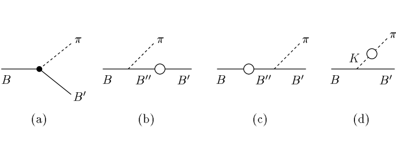
FIG. 1.: Diagrams contributing to the $P$-wave decays: (a) contact contribution, (b), (c) baryon pole contributions, (d) kaon pole contribution.

REFERENCES

- [1] J.F. Donoghue, E. Golowich and B. R. Holstein, Phys. Rep. 131, 319 (1986)
- [2] E. Jenkins, Nucl. Phys. B375, 561 (1992); R.P. Springer, Phys. Lett. B461, 167 (1999); B. Borasoy and B.R. Holstein, Phys. Rev. D59, 094025 (1999); A. Abd El-hady and J. Tandean, hep-ph/9908498
- [3] E.M. Henley, W-Y.P. Hwang and L.S. Kisslinger, hep-ph/9912530
- [4] J.F. Donoghue, E. Golowich and Y-C. R. Lin, Phys. Rev. D32, 1733 (1985); D33, 2728(E) (1986)
- [5] M. Praszalowicz, Phys. Lett. 158B, 264 (1985); M. Chemtob, Nucl. Phys. B256, 600 (1985)
- [6] M. Praszalowicz and J. Trampetic, Phys. Lett. 161B, 169 (1985)
- [7] H. Weigel, Int.J.Mod.Phys.A11, 2419 (1996)
- [8] N.N. Scoccola, Phys. Lett. B428, 8 (1998)
- [9] N. Toyota and K. Fujii, Prog. Theor. Phys. 75, 340 (1986); N. Toyota, Prog. Theor. Phys. 77, 688 (1987)
- [10] Y. Kondo, S. Saito and T. Otofuji, Phys. Lett. B236, 1 (1990)
- [11] H. Yabu and K. Ando, Nucl. Phys. B301, 601 (1988)
- [12] J. Kambor, J. Missimer and D. Wyler, Nucl. Phys. B346, 17 (1990)
- [13] J. Kambor, J. Missimer and D. Wyler, Phys. Lett. B261, 496 (1991)
- [14] J.F. Donoghue, E. Golowich and B. R. Holstein, Phys. Rev. D30, 587 (1984)
- [15] G. Ecker, J. Kambor and D. Wyler, Nucl. Phys. B394, 101 (1993)
- [16] E. Golowich, Phys. Rev. D35, 2764 (1987)
- [17] E. Golowich, Phys. Rev. D36, 3516 (1987)
- [18] J.F. Donoghue, E. Golowich and B. R. Holstein, Dynamics of the Standard Model (Cambridge Univ. Press, Cambridge, 1994)
- [19] Ulf–G. Meißner and H. Weigel, Phys. Lett. B447, 1 (1999)
- [20] J.J. de Swart, Rev. Mod. Phys. 35, 916 (1963); P. McNamee, S.J. and F. Chilton, Rev. Mod. Phys. 36, 1005 (1964)