hep-ph/0001039
          CERN-TH/2000-002
          FTUV/99-71
          IFIC/99-74

Supernova Bounds on Majoron-emitting decays of light neutrinos
M. Kachelrieß^1,2, R. Tomàs² and J. W.F. Valle^2
1 TH Division, CERN, CH-1211 Geneva 23

² Institut de Física Corpuscular – C.S.I.C.

Departament de Física Teòrica – Univ. de València

Edifici Instituts de Paterna – Apartat de Correus 2085 – 46071, València

http://neutrinos.uv.es

1 Introduction

The solar [1] and atmospheric [2] neutrino problems have provided two milestones in the search for physics beyond the Standard Model, giving strong evidence for $\nu_{e}$ and $\nu_{\mu}$ conversions, respectively. Although flavour changing neutral current interactions (FCNC) [3, 4, 5] and/or neutrino decays [6] may play an important rôle in the interpretation of the data [7, 8, 9], we concentrate here on oscillations involving very small neutrino mass splittings, because they provide the simplest picture [10, 11, 12]. Moreover, reconciling the LSND data [13] and/or hot dark matter suggests the existence of a light sterile neutrino [14]. Pending the confirmation of LSND results by future experiments, we choose however to use in this work just the solar and atmospheric data assuming the absence of sterile neutrinos, FCNC and/or of heavier neutrinos.

Within the simplest extensions of the Standard Model in which neutrino masses are introduced by an explicit breaking of lepton–number via the seesaw mechanism there are neutral-current-mediated neutrino decays $\nu^{\prime}\to 3\nu$ [3], but these decays are extremely slow for the neutrino masses of interest for us here. If neutrino masses arise from the spontaneous violation of ungauged lepton number, the corresponding Goldstone boson [15] brings in the possibility of new, potentially faster, 2-body neutrino decays [6],

$$\nu^{\prime}\to\nu+J\>.$$ (1)

However it is well-known that in the simplest well–motivated majoron models the neutrino mass and coupling matrices are proportional, so that decays are highly suppressed in vacuo [16]. As a result, neutrino decays become cosmologically and astrophysically irrelevant in these models. Moreover, for the small masses indicated by solar and atmospheric neutrino data, the annihilation channels $\nu^{\prime}+\nu^{\prime}\to J+J$ are also negligible.

The purpose of the present work is to discuss the possible impact of neutrino-majoron interactions on the supernova (SN) neutrino signal. Together with the early Universe SN are the only site where neutrinos are in thermal equilibrium and so abundant that neutrino-neutrino interactions become important. Therefore, SN physics has been one of the main tools to derive limits on neutrino parameters in majoron models [18, 19, 20, 21].

The arguments used in the literature can be divided mainly into two classes: The first uses the fact that majoron interactions violate lepton number (like in $\nu\to\bar{\nu}+J$ or $\nu+\nu\to\bar{\nu}+\bar{\nu}$) and, thereby, can reduce the trapped electron lepton number fraction $Y_{L_{e}}$ in the SN core [18, 19]. Since in several SN simulations it was found that a minimum value of $Y_{L_{e}}\raise 1.29167pt\hbox{$\;>$\kern-7.5pt\raise-4.73611pt\hbox{$\sim\;$}}0.38$ is needed in order to have a successful bounce shock, the strength of the lepton number violating interactions can be correspondingly restricted. Unfortunately, the older works [18] using this argument did not take into account the derivative nature of the coupling of a Goldstone boson calculating the scattering cross sections. Moreover, an approximation valid only in vacuum was used for the neutrino decay rates. In ref. [19] the correct medium decay rates were used for the first time, giving the stringent limit $g_{ee}\raise 1.29167pt\hbox{$\;<$\kern-7.5pt\raise-4.73611pt\hbox{$\sim\;$}}5\times 10^{-6}$.

The second argument used is a “classical” energy loss argument: the observed neutrino signal of SN 1987A should not be shortened too much by additional majoron emission [19, 20, 21]. The most comprehensive work along this line is Ref. [21] which also uses the correct derivative coupling of the majoron. The limits found there depend on the value of the $(B-L)$ breaking scale. For example the range $5\times 10^{-7}\raise 1.29167pt\hbox{$\;<$\kern-7.5pt\raise-4.73611pt\hbox{$\sim\;$}}g\raise 1.29167pt\hbox{$\;<$\kern-7.5pt\raise-4.73611pt\hbox{$\sim\;$}}6\times 10^{-5}$ is excluded for $v=20$ GeV while $1\times 10^{-5}\raise 1.29167pt\hbox{$\;<$\kern-7.5pt\raise-4.73611pt\hbox{$\sim\;$}}g\raise 1.29167pt\hbox{$\;<$\kern-7.5pt\raise-4.73611pt\hbox{$\sim\;$}}7\times 10^{-5}$ is excluded for $v=500$ GeV. The tau-neutrino masses considered in Ref. [21] are, compared to the values currently discussed, rather large, 100 eV $\raise 1.29167pt\hbox{$\;<$\kern-7.5pt\raise-4.73611pt\hbox{$\sim\;$}}m_{\nu_{\tau}}\raise 1.29167pt\hbox{$\;<$\kern-7.5pt\raise-4.73611pt\hbox{$\sim\;$}}30$ MeV. It is therefore of certain interest to extend their discussion to lower neutrino masses presently indicated by the solutions to the solar and atmospheric neutrino anomalies.

These astrophysical limits should be confronted with the available laboratory constraints. While there is a stringent limit from $\beta\beta$ experiments [22],

$$\sum_{i,j}g_{ij}U_{ei}U_{ej}\raise 1.29167pt\hbox{$\;<$\kern-7.5pt\raise-4.73611pt\hbox{$\sim\;$}}3\times 10^{-5}\,,$$ (2)

the limits from pion [23] and kaon decays [24] are rather weak,

$$\sum_{l=e,\mu,\tau}g_{el}^{2}\raise 1.29167pt\hbox{$\;<$\kern-7.5pt\raise-4.73611pt\hbox{$\sim\;$}}3\times 10^{-5}\quad{\rm and}\quad\sum_{l=e,\mu,\tau}g_{\mu l}^{2}\raise 1.29167pt\hbox{$\;<$\kern-7.5pt\raise-4.73611pt\hbox{$\sim\;$}}2.4\times 10^{-4}\,.$$ (3)

Note also that individual couplings $g_{ij}$ could be larger than the limit from $\beta\beta$ experiments due to possible cancellations [25].

The main purpose of the present work is the study of the impact of neutrino-majoron interactions on the observable neutrino signal of a supernova. Since decays of the type $\bar{\nu}_{e}\to\nu_{l}+J$ reduce the $\bar{\nu}_{e}$ flux, a limit on the neutrino majoron coupling constants can be derived from the observed signal of SN 1987A. In so–doing one must include in the analysis the fact that massive neutrinos may oscillate on their way from the SN envelope to the detector. We do that and present the excluded regions for the three currently discussed solutions of the solar neutrino problem  [10, 11]. Then we estimate the discovery potential of new experiments like Superkamiokande (SK) and the Sudbury Neutrino Observatory (SNO) in the case of a future galactic supernova. We find that these experiments could probe majoron neutrino coupling constants $g$ down to $g\raise 1.29167pt\hbox{$\;>$\kern-7.5pt\raise-4.73611pt\hbox{$\sim\;$}}\mathrm{few}\times 10^{-5}$.

2 Matter effect on neutrino-majoron interactions

We consider the simplest class of models in which neutrinos acquire mass from the spontaneous violation of ungauged lepton number [15]. In this case it is well-known that the massless Goldstone boson $J$ – the majoron – couples diagonally to the mass-eigenstate neutrinos $\nu_{i}$ to a very good approximation [16]. In other words, after rotation from the weak basis $\nu_{\alpha}$ through $\theta_{0}$ angle(s) the original coupling matrix $g_{\alpha\beta}$ transforms into

$$g_{ij}\approx\delta_{ij}g_{i}\,.$$ (4)

We denote by $\nu_{i}^{(h_{i})}$ the 4-spinor describing the majorana neutrino with mass $m_{i}$ and helicity $h=\pm 1$.

In this section, we briefly review the effect of a thermal background on the neutrino majoron interactions. It was first demonstrated by Berezhiani and Vysotsky in Ref. [26] that the effective mass induced by the interactions of neutrinos with background matter can break the proportionality between the mass matrix $m_{ij}$ and the coupling matrix $g_{ij}$ characteristic of the simplest majoron models in vacuo [16]. A thermal background consists, except in the early Universe, only of particles of the first generation and, therefore distinguishes the electron flavour from the other flavours.

In Ref. [26], the Lagrangian describing neutrino majoron interaction in a thermal background was obtained in a relativistic approximation similar to the usual treatment of neutrino oscillations in matter. Later, the authors of Ref. [29] solved this problem without using this approximation and confirmed the results of Ref. [26] in the appropriate limiting cases. Here we are concerned with SN neutrinos, which have typical energies around $10-25$ MeV. Therefore, we will take advantage of the simpler relativistic approximation and we will follow closely Ref. [26].

The Hamiltonian $H_{\rm tot}\equiv H(x)$ describing the evolution of neutrinos may be given as

$$H_{\rm tot} = H_{0}+H_{\rm med}+H_{\rm int}$$ (5)

$$= H_{0}+\sum_{i,j}\sum_{h_{i},h_{j}}\bar{\nu}_{i}^{(h_{i})}V_{ij}^{h_{i},h_{j}}\nu_{j}^{(h_{j})}+g_{ij}\bar{\nu}_{i}^{(h_{i})}\gamma_{5}\nu_{j}^{(h_{j})}J\,,$$ (6)

where the free Hamiltonian $H_{0}$ describes the propagation in vacuo, $H_{\rm med}$ describes the effects of matter and $H_{\rm int}$ takes into account the presence of neutrino-majoron interactions which may lead to decays. Instead of using the eigenstates of the free Hamiltonian $H_{0}$ as basis for perturbation theory, we will use the eigenstates of $H_{0}+H_{\rm med}$. Therefore, as a first step the Dirac equation, $(H_{0}+V)\nu_{j}^{(\pm)}=i\partial_{t}\nu_{j}^{(\pm)}$ has to be solved. In the case of ultra-relativistic neutrinos, it is well-known that a vector-like potential does not change the helicity of the neutrinos — its only effect is a rotation of the eigenstates of $H_{0}+V$ with respect to the mass basis [30]. Therefore, the Dirac equation simplifies and reduces to the standard form known from neutrino oscillations,

$$i\partial_{t}\nu_{i}^{(h)}=(H^{\rm rel}_{ij}+U_{i\alpha}V_{\alpha\beta}U^{\dagger}_{\beta j})\nu_{j}^{(h)}$$ (7)

where $H^{\rm rel}_{ij}\approx(p+m_{i}^{2}/(2p))\delta_{ij}$ and $V_{\alpha\beta}$ is the potential matrix in the weak basis

$$V_{\alpha\beta}=\left(\begin{array}[]{ccc}V_{C}+V_{N}&0&0\\ 0&V_{N}&0\\ 0&0&V_{N}\end{array}\right)\,.$$ (8)

The potentials induced by the charged and neutral currents are $V_{C}=\sqrt{2}hG_{F}n_{B}(Y_{e}+Y_{\nu_{e}})$ and $V_{N}=\sqrt{2}hG_{F}n_{B}\left(-\frac{1}{2}Y_{N}+Y_{\nu_{e}}\right)$, where $Y_{i}=(n_{i}-n_{\bar{i}})/n_{B}$ and $n_{B}$ is the baryon density. Finally, $U$ is the mixing matrix relating mass and weak basis and defined through $\nu_{i}=U_{i\alpha}\nu_{\alpha}$. Diagonalizing $H^{\rm rel}+UVU^{\dagger}$ gives the medium states $\tilde{\nu}_{i}^{(h)}=\tilde{U}_{ij}^{(h)}\nu_{j}^{(h)}$.

In the case of a two-flavor neutrino system the mixing matrices, $U$ and $\tilde{U}$, can be parametrized by $\theta_{0}$ and $\theta^{(h)}$ respectively. The diagonalization of the Hamiltonian leads us to the following expression for the effective mixing angle,

$$\sin^{2}2\theta^{(\pm)}(p)=\frac{\sin^{2}2\theta_{0}}{\sin^{2}2\theta_{0}+(\cos 2\theta_{0}-\xi^{(\pm)})^{2}}\>,$$ (9)

where

$$\xi^{(h)}=h\>\frac{\Delta_{0}}{2p\;G_{F}(Y_{e}+Y_{\nu_{e}})n_{B}}\>,$$ (10)

and $\Delta_{0}=m_{2}^{2}-m_{1}^{2}$. The effective masses in the medium are

$$m_{1,2}^{(h)\;2}=-hp(2V_{N}+V_{C})+\frac{1}{2}(m_{1}^{2}+m_{2}^{2})\mp\frac{1}{2}\Delta^{(h)}\>,$$ (11)

where the upper sign is for $m_{1}$, the lower for $m_{2}$ and

$$\Delta^{(h)}=\sqrt{(\Delta_{0}\cos 2\theta_{0}+2hpV_{C})^{2}+(\Delta_{0}\sin 2\theta_{0})^{2}}\>.$$ (12)

For typical neutrino energies and densities near the neutrino–spheres, the parameter

$$\xi=6.53\times 10^{-8}\frac{\Delta_{0}}{10^{-3}{\rm eV}^{2}}\;\frac{10{\rm MeV}}{p}\;\frac{10^{10}{\rm g/cm}^{-3}}{(Y_{e}+Y_{\nu_{e}})\rho}$$ (13)

is much smaller than one. This fact will give rise to the following simplification, $\theta^{(+)}(p)\approx-\theta_{0}$ and $\theta^{(-)}(p)\approx\pi/2-\theta_{0}$, which, as it will be shown later, will allow us to identify medium and weak interaction states.

In the three-flavor neutrino case the mixing matrix $U$ can be parametrized as $U=U_{12}U_{13}U_{23}U_{0}$, where the matrices $U_{ij}=U_{ij}(\theta_{ij})$ perform the rotation in the $ij$-plane by the angle $\theta_{ij}$ and $U_{0}$ includes possible CP-violation effects [3]. In the following we will assume for simplicity CP conservation and $\theta_{13}=0$, the latter motivated both by detailed fits of the atmospheric neutrino anomaly, but also by the results of the Chooz experiment [27]. This simplifies the mixing matrix to $\nu_{i}=U_{i\alpha}\nu_{\alpha}=U_{12}U_{23}\nu_{\alpha}$ [28] and we can make the assignment, $\theta_{12}=\theta_{\odot}$ and $\theta_{23}=\theta_{\rm atm}$. Notice that for light neutrinos near the neutrino spheres the condition $|V_{\alpha\alpha}|\gg m_{i}^{2}/(2p)$ ($\xi\ll 1$) holds and, since in the weak basis the potential is diagonal, the medium states can be identified with the weak ones up to a rotation in the $\nu_{\mu}-\nu_{\tau}$ subspace. The expressions can be simplified by choosing this arbitrary rotation angle to coincide with $\theta_{23}$. Then, only one angle, $\theta^{(h)}$, will be required to connect medium and mass eigenstates, and one will be able to recover the two-flavor neutrino case,

$$\tilde{\nu}_{i}^{(h)}=\tilde{U}_{ij}^{(h)}\nu_{j}^{(h)}=\tilde{U}_{ij}(\theta^{(h)})\nu_{j}^{(h)}=\left\{\begin{array}[]{lcl}\tilde{\nu}_{i}^{(+)}&=&\tilde{U}_{ij}(-\theta_{12})~{}~{}\nu_{j}^{(+)}\\ \tilde{\nu}_{i}^{(-)}&=&\tilde{U}_{ij}(\pi/2-\theta_{12})~{}\nu_{j}^{(-)}\\ \end{array}\right.\,.$$ (14)

Thus the medium states can be identified with weak interaction states according to Table 1 and the coupling matrix $\tilde{g}_{ij}$ in the medium basis can be approximated by the one in the weak basis, $g_{\alpha\beta}$.

medium state	weak state	potential
$\tilde{\nu}_{1}^{(+)}$	$\bar{\nu}_{e}$	$-(V_{C}+V_{N})$
$\tilde{\nu}_{2}^{(+)}$	$c_{23}\bar{\nu}_{\mu}+s_{23}\bar{\nu}_{\tau}$	$-V_{N}$
$\tilde{\nu}_{3}^{(+)}$	$-s_{23}\bar{\nu}_{\mu}+c_{23}\bar{\nu}_{\tau}$	$-V_{N}$
$\tilde{\nu}_{1}^{(-)}$	$c_{23}\nu_{\mu}+s_{23}\nu_{\tau}$	$V_{N}$
$\tilde{\nu}_{2}^{(-)}$	$\nu_{e}$	$V_{C}+V_{N}$
$\tilde{\nu}_{3}^{(-)}$	$-s_{23}\nu_{\mu}+c_{23}\nu_{\tau}$	$V_{N}$

Table 1: Medium eigenstates $\tilde{\nu}_{i}^{\pm}$, equivalent weak eigenstates in the limit $\xi\ll 1$ and their potential energy $V=m^{(\pm)2}/(2p)$.

Above, we have derived the transformation matrix $U_{ij}(\theta^{(\pm)})$ between mass and medium eigenstates. The relation between the corresponding coupling matrices in vacuo $g_{if}$ and in medium $\tilde{g}_{if}$ is given by

$$\tilde{g}_{if}^{h_{i}\to h_{f}}=\tilde{U}_{in}(\theta^{(h_{i})})g_{nm}\tilde{U}_{mf}^{T}(\theta^{(h_{f})})=\left(\begin{array}[]{ccc}c_{f}c_{i}\,g_{11}+s_{f}s_{i}\,g_{22}&s_{i}c_{f}\,g_{22}-c_{i}s_{f}\,g_{11}&0\\ c_{i}s_{f}\,g_{22}-s_{i}c_{f}\,g_{11}&s_{f}s_{i}\,g_{11}+c_{f}c_{i}\,g_{22}&0\\ 0&0&g_{33}\end{array}\right)$$ (15)

with $c_{i,f}=\cos[\theta^{(\pm)}(p_{i,f})]$ and $s_{i,f}=\sin[\theta^{(\pm)}(p_{i,f})]$. Notice that the coupling constant $g_{33}$ will only appear in decays not involving electron neutrinos or anti–neutrinos, so that it will not be important for us.

Within our relativistic approximation, only helicity–flipping neutrino decays $\nu_{i}^{\pm}\to\nu_{j}^{\mp}+J$ occur. For these decays, the differential decay rate is

$$\frac{d\Gamma}{dp_{f}}=\frac{\tilde{g}_{if}^{2}}{8\pi}\left(\frac{p_{i}-p_{f}}{p_{i}^{2}}\right)\left(\frac{m_{i}^{(\pm)2}}{2p_{i}}-\frac{m_{f}^{(\pm)2}}{2p_{f}}\right)\>.$$ (16)

In the next section, we will apply this formula to supernova. Additional simplifications of the limit $\xi\ll 1$ are in this case $m_{i,f}^{(\pm)2}/(2p_{i,f})=V_{i,f}$ and that the coupling constants do not depend on $p_{i,f}$. Hence, we can integrate Eq. (16) and obtain as total decay rate

$$\Gamma=\frac{\tilde{g}_{if}^{2}}{16\pi}(V_{i}-V_{f})$$ (17)

and as average energy of the final neutrino $\langle E_{f}\rangle=E_{i}/3$. Obviously, only those decays are possible for which $V_{i}-V_{f}>0$.

Besides enhancing the rates for neutrino decay, the dispersive effects of the medium open also completely new decay channels of the majoron into neutrinos [31]. The majoron decays $J\to\nu_{i}^{\pm}+\nu_{j}^{\pm}$ have the same matrix elements like the neutrino decays $\nu_{i}^{\mp}\to\nu_{j}^{\pm}+J$ considered above. Their total decay rate is [31]

$$\Gamma=\frac{\tilde{g}_{ij}^{2}}{8\pi}(-V_{i}-V_{j})\>S$$ (18)

and now those decays are possible for which $V_{i}+V_{j}<0$. The symmetry factor $S$ is $S=1/2$ if the two neutrinos are identical, and $S=1$ otherwise. Finally, we note that the neutrinos are emitted isotropically.

3 Supernova neutrinos and neutrino majoron decays

Here we first collect the available limits on majoron neutrino coupling constants from the observation of the neutrino signal of SN 1987A and comment on their validity. Then, we discuss the sensitivity of new experiments like SK or SNO to probe neutrino-majoron interactions in the case of a future galactic supernova.

3.1 Constraints from collapsing phase

Massive stars become inevitably unstable at the end of their life, when their iron core reaches the Chandrasekhar limit. The collapse of the iron core is only intercepted when nuclear density, $\rho_{0}\approx 3\times 10^{14}$ g/cm³, is reached. At this point, the implosion is turned into an explosion: a shock wave forms at the edge of the core and moves outward. The strength of this bounce shock and its successful propagation is extremely sensitive to the trapped electron lepton fraction $Y_{L_{e}}=Y_{e}+Y_{\nu_{e}}$, attained by the core during its infall. A successful SN explosion occurs only if at least 90% of the initial $Y_{L_{e}}$ is still present [32], which translates to $Y_{L}(t_{\rm bounce})\raise 1.29167pt\hbox{$\;>$\kern-7.5pt\raise-4.73611pt\hbox{$\sim\;$}}0.375$ [33].

We now use this requirement in order to derive a limit on majoron decays. Such decays clearly change $Y_{L_{e}}$ either by two units ($\nu_{e}\to\bar{\nu}_{e}+J$) or by one ($\nu_{e}\to\bar{\nu}_{\mu}+J$). Since the allowed change in $Y_{L}$ is small, we can still use the profiles $Y_{e}(t)$ and $Y_{\nu_{e}}(t)$ from a “standard” SN simulation [34]. One can easily check from Table 1 that only the first of the above decays takes place, since $Y_{e}+3/2Y_{\nu_{e}}<1/2$. Hence the deleptonization rate is governed by

$$\frac{dY_{L,{\rm decays}}}{dt}=-2\Gamma(\nu_{e}\to\bar{\nu}_{e}+J)Y_{\nu_{e}}\,.$$ (19)

We integrate Eq. (19) numerically from $t_{0}$, the time when neutrinos start to become trapped (at $\rho(t_{0})\approx 5\times 10^{11}$ g/cm³), to the time of the bounce $t_{\rm bounce}$. Note that in the numerical simulation [34] whose results we are using $Y_{L}$ increases from $Y_{L}(t_{0})\approx 0.37$ up to $Y_{L}(t_{\rm bounce})\approx 0.39$. Requiring that $Y_{L}(t_{\rm bounce})>0.375$ [32, 33], i.e. $|\Delta Y_{L,{\rm decays}}|<0.015$, we obtain

$$g_{ee}=g_{11}\cos^{2}\theta_{0}+g_{22}\sin^{2}\theta_{0}\raise 1.29167pt\hbox{$\;<$\kern-7.5pt\raise-4.73611pt\hbox{$\sim\;$}}2\times 10^{-6}\,.$$ (20)

Using the same argument, the limit $g_{ee}\raise 1.29167pt\hbox{$\;<$\kern-7.5pt\raise-4.73611pt\hbox{$\sim\;$}}5\times 10^{-6}$ was derived in Ref. [19].

This limit relies on numerical modeling of SN explosions, in particular on the success of the explosion in specific models. However, it is probably fair to say that current supernova models have generally problems to produce successful explosions. Therefore, Eq. (20) cannot be viewed as a trustworthy limit as long we do not have a better understanding of SN dynamics.

3.2 Constraints from majoron luminosity

Numerical computations [35] of the total amount of binding energy $E_{b}$ released in a supernova explosion yield, within a plausible range of progenitor star masses and somewhat depending on the equation of state used,

$$E_{b}=(1.5-4.5)\times 10^{53}\>{\rm erg}\,.$$ (21)

This range of values is confirmed by likelihood analysis of the observed $\bar{\nu}_{e}$ spectrum of SN 1987A under the hypothesis of small mixing of $\bar{\nu}_{e}$ with other neutrino flavours [36]. Therefore, the parameter space of models which give rise to majoron luminosity large enough that the observed $\bar{\nu}_{e}$ signal is significantly shortened can be restricted. The most comprehensive analysis of SN cooling and majoron emission using this argument was given in Ref. [21].

Our following analysis has three main differences compared to Ref. [21]: First, we are interested in relatively light neutrinos ($m^{2}\raise 1.29167pt\hbox{$\;<$\kern-7.5pt\raise-4.73611pt\hbox{$\sim\;$}}{\rm eV}^{2}\ll 2pV$) as suggested by the simplest interpretation of data from solar and atmospheric neutrino experiments. Therefore, medium effects become important not only for decays like $\nu\to\nu^{\prime}+J$ but also for scattering processes like $J+\nu\to J+\nu$. Second, we do not include the process $J+J\to J+J$ in the calculation of the majoron opacity. A discussion of why self-scattering processes do not contribute to the opacity was given in Ref. [37] for the case of $\nu+\nu\to\nu+\nu$ scattering. Note that trapping due to $J+J\to J+J$ scattering prevented Choi and Santamaria from excluding majoron–neutrino couplings for the case of light neutrino masses, $m_{\nu_{\tau}}\raise 1.29167pt\hbox{$\;<$\kern-7.5pt\raise-4.73611pt\hbox{$\sim\;$}}100$ eV. Third, we calculate the majoron luminosity in the trapping regime in a different way.

Let us discuss first the mean free path of majorons. The main source of opacity for majorons are the processes $J+J\to\nu+\nu$, $J+\nu\to J+\nu$, and $J+\nu\to\nu$ (cf. [21]). Taking into account the effective mass of the neutrinos, the corresponding mean free paths inside the SN core with radius $r_{0}\sim 10$ km and density $\rho\sim\rho_{\rm nuc}$ are given by,

$$l^{-1}(J+J\to\nu+\nu) = 1.9\times 10^{18}g^{4}\left(\frac{{\rm keV}}{m_{\rm eff}}\right)^{2}\left(\frac{T}{25\rm MeV}\right)^{3}{\rm cm}^{-1}$$ (22)

$$l^{-1}(J+\nu\to J+\nu) = 1.5\times 10^{18}g^{4}\left(\frac{{\rm keV}}{m_{\rm eff}}\right)^{2}\left(\frac{T}{25\rm MeV}\right)^{3}{\rm cm}^{-1}$$ (23)

$$l^{-1}(\nu+J\to\nu) = 1\times 10^{4}g^{2}\;\left(\frac{T}{25\rm MeV}\right){\rm cm}^{-1}\,.$$ (24)

For the effective neutrino mass inside the SN core, $m_{\rm eff}^{2}\sim 2pV$, we use $m_{\rm eff}\sim 20$ keV. Requiring that the mean free path of the majorons is $\raise 1.29167pt\hbox{$\;>$\kern-7.5pt\raise-4.73611pt\hbox{$\sim\;$}}10$ km, we obtain that they escape freely for $g\raise 1.29167pt\hbox{$\;<$\kern-7.5pt\raise-4.73611pt\hbox{$\sim\;$}}3\times 10^{-6}$.

Next, we consider the luminosity for the case that majorons are not trapped. Then they are emitted by the whole core volume with luminosity

$${\cal L}(\nu+\nu\to J+J) = 5.5\times 10^{80}g^{4}\left(\frac{\rm keV}{m_{\rm eff}}\right)^{2}{\rm erg/s}$$ (25)

$${\cal L}(\nu\to\nu+J) = 4.8\times 10^{65}g^{2}\;{\rm erg/s}\,.$$ (26)

We require now that the majoron luminosity during 10 s does not exceed the maximal theoretical value of the binding energy, ${\cal L}_{J}\raise 1.29167pt\hbox{$\;<$\kern-7.5pt\raise-4.73611pt\hbox{$\sim\;$}}5\times 10^{52}$erg/s, and obtain the limit $g\raise 1.29167pt\hbox{$\;<$\kern-7.5pt\raise-4.73611pt\hbox{$\sim\;$}}3\times 10^{-7}$. In the trapping regime, the energy loss argument therefore excludes the band

$$3\times 10^{-7}\raise 1.29167pt\hbox{$\;<$\kern-7.5pt\raise-4.73611pt\hbox{$\sim\;$}}g\raise 1.29167pt\hbox{$\;<$\kern-7.5pt\raise-4.73611pt\hbox{$\sim\;$}}3\times 10^{-6}$$ (27)

for vacuum neutrino masses $m\ll m_{\rm eff}\sim 20$ keV.

Let us now discuss the case that majorons are trapped, $g\raise 1.29167pt\hbox{$\;>$\kern-7.5pt\raise-4.73611pt\hbox{$\sim\;$}}3\times 10^{-6}$. We recall first the standard treatment as presented, e.g., in Ref. [21]. The main assumption is that ${\cal L}_{J}$ can be approximated by blackbody surface emission

$${\cal L}_{J}=\frac{\pi^{3}}{30}R_{J}^{2}T^{4}$$ (28)

of a thermal majoron–sphere which radius $R_{J}$ is defined to be at optical depth 2/3,

$$\int_{R_{J}}^{\infty}dr\>l^{-1}(r)=\frac{2}{3}\,.$$ (29)

Assuming furthermore a temperature profile $T(r)$ outside the supernova core, one can determine for which range of coupling constants ${\cal L}_{J}$ exceeds a certain critical value.

There are two shortcomings in this argumentation. First, the profile $T(r)\propto r^{-2}$ used for $r>r_{0}$ in [21] represents the temperature of ordinary matter (nucleons, $e^{\pm}$, photons). However, majorons couple mainly to neutrinos and would at best be in thermal equilibrium with neutrinos, if at all, but not with nucleons. Second, the use of Eqs. (22-24) which were derived for isotropic distributions inside the core is not justified for the highly non–isotropic distributions outside the neutrino– or majoron–spheres. Using for the density $n_{i}(r)$ of a particle species $i$ with sphere radius $R_{i}$ the expression

$$n_{i}(r)=\frac{{\cal L}_{i}}{\langle E_{i}\rangle}\frac{1}{4\pi r^{2}}\,,$$ (30)

and introducing the additional factor $\langle 1-\cos\theta\rangle\sim(R_{i}/r)^{2}$ which represents the averaging over the angle $\theta$ between the momenta of the radially outgoing test majoron and the particle $i$ in the mean free path one finds that $n_{i}(r)\propto 1/r^{4}$. This renders support to our claim that there is a sharp drop in the majoron opacity in crossing the neutrino spheres. Note also that it was recently stressed in Ref. [38] that a naive application of the Stefan-Boltzmann law can be dangerous for the calculation of neutrino–sphere radii.

We prefer therefore not to rely on the argumentation presented above. Instead, we calculate the volume rather than the surface luminosity, but taking into account that only majorons emitted from the shell $[r_{0}-l:r_{0}]$ can escape [19]. We find that the majoron luminosity drops below ${\cal L}_{\nu,{\rm tot}}\sim E_{b}/10$ s for $g\raise 1.29167pt\hbox{$\;>$\kern-7.5pt\raise-4.73611pt\hbox{$\sim\;$}}2\times 10^{-5}$. Going even to larger values of $g$, majorons and neutrinos are becoming so strongly coupled that it is reasonable to assume that the SN core emits roughly the same luminosity in form of majorons as in one neutrino species, ie. ${\cal L}_{J}\sim{\cal L}_{\nu,{\rm tot}}/6$. Therefore, majoron emission in this regime is not constrained at all by the energy loss argument. Combining the both limits obtained, majoron couplings one concludes that the range

$$3\times 10^{-7}\raise 1.29167pt\hbox{$\;<$\kern-7.5pt\raise-4.73611pt\hbox{$\sim\;$}}g\raise 1.29167pt\hbox{$\;<$\kern-7.5pt\raise-4.73611pt\hbox{$\sim\;$}}2\times 10^{-5}$$ (31)

is excluded for vacuum neutrino masses $m\ll m_{\rm eff}\sim 20$ keV.

A final remark is in order. We have been using rather loosely only one coupling constant $g$ in this section. More precisely, we mean by $g$ the element of the coupling matrix $g_{\alpha\beta}$ in the weak basis with the largest absolute value.

3.3 Constraints from neutrino spectra

During the Kelvin-Helmholtz cooling phase, $t\approx 1-10$ s after core bounce, the protoneutron star slowly contracts and cools by neutrino emission. The neutrino luminosities are governed by the energy loss of the core and are, therefore, approximately equal for each type of (anti-) neutrinos. Since the opacity of, e.g., $\bar{\nu}_{\mu,\tau}$ is smaller than of $\bar{\nu}_{e}$, due to their smaller cross section, their energy-exchanging reactions already freeze out in the denser part of the protoneutron star. Hence, one expects the spectral temperatures of $\bar{\nu}_{e}$ to be smaller than the one of $\nu_{h}=\{\nu_{\mu,\tau},\bar{\nu}_{\mu,\tau}\}$. Typically, the average energies $\langle E_{i}\rangle$ found in simulations [39] are

$$\langle E_{\nu_{e}}\rangle\approx 11~{}{\rm MeV}\,,\qquad\langle E_{\bar{\nu}_{e}}\rangle\approx 16\;{\rm MeV}\,,\qquad\langle E_{\nu_{h}}\rangle\approx 25~{}{\rm MeV}\,.$$ (32)

It is convenient to define three energy spheres $R_{E,\nu_{e}}$, $R_{E,\bar{\nu}_{e}}$ and $R_{E,\nu_{h}}$, outside of which only energy-conserving reactions contribute to the neutrino opacity. These reactions, mainly neutral current neutrino-nucleon and neutrino-nucleus scattering, do not change the neutrino spectra, although the neutrinos still undergo several scattering as they diffuse outward. Eventually, the neutrinos reach the transport sphere at $R_{t,\nu_{i}}$, where also the energy-conserving reactions freeze out, and escape freely. This sphere, i.e. the surface of last scattering, is what most authors mean with “the” neutrino–sphere.

For the numerical evaluation of the decay rates, we use profiles for $\rho(r)$ and $Y_{e}(r)$ from Wilson’s SN model [40] at the time $t=6$ s after core bounce. For all radii of interest, only anti-neutrinos can decay into neutrinos. Correspondingly, the allowed majoron decay channels can be determined from Table 1. For the average position of the various neutrino–spheres, we use the implicit definition

$$\rho(R_{E,\nu_{h}})=2\times 10^{13}{\rm g/cm}^{3}\,,\qquad\rho(R_{E,\bar{\nu}_{e}})=2\times 10^{12}{\rm g/cm}^{3}\,,\qquad\rho(R_{E,\nu_{e}})=2\times 10^{11}{\rm g/cm}^{3}\,,$$ (33)

and

$$\rho(R_{T,\nu_{h}})=\rho(R_{T,\bar{\nu}_{e}})=\rho(R_{T,\nu_{e}})=2\times 10^{11}{\rm g/cm}^{3}\,.$$ (34)

In calculating the effect of majoron–emitting neutrino decays on the emitted $\nu$ spectra we must distinguish three regions. If a $\bar{\nu}_{i}$ is produced inside its own energy sphere, $r<R_{E,\bar{\nu}_{i}}$, it is still in thermal and chemical equilibrium with the stellar medium. Therefore, the production (or the decay) of a $\bar{\nu}_{i}$ within $r<R_{E,\bar{\nu}_{i}}$ does not influence the emitted $\bar{\nu}_{i}$ spectrum. In contrast, the spectrum of $\bar{\nu}_{i}$ neutrinos is fixed for $r>R_{E,\bar{\nu}_{i}}$ and both its decay or its production changes its spectra. The only difference between the two regions $R_{E,\bar{\nu}_{i}}<r<R_{t,\bar{\nu}_{i}}$ and $r>R_{t,\bar{\nu}_{i}}$ is the different “effective” velocity $v$ of the decaying neutrino. In the latter, the neutrino can escape freely ($v=1$), while in the first it diffuses outward with $v\approx\lambda/(R_{E,\bar{\nu}_{i}}-R_{t,\bar{\nu}_{i}})$. Here, $\lambda$ is the average mean free path of the neutrino $\bar{\nu}_{i}$. Hence, we can compute the survival probability $N(\bar{\nu}_{i})$ of a $\bar{\nu}_{i}$ neutrino emitted from its energy sphere as

$$N(\bar{\nu}_{i})=\exp\left\{-\int_{R_{E,\bar{\nu}_{i}}}^{R_{t,\bar{\nu}_{i}}}\frac{dr^{\prime}}{v}\>\Gamma_{\bar{\nu}_{i}}(r^{\prime})-\int_{R_{t,\bar{\nu}_{i}}}^{\infty}dr^{\prime}\>\Gamma_{\bar{\nu}_{i}}(r^{\prime})\right\}\,,$$ (35)

where

$$\Gamma_{\bar{\nu}_{i}}=\sum_{l=e,\mu,\tau}\Gamma(\bar{\nu}_{i}\to\nu_{l}+J)$$ (36)

is its total decay rate. Denoting with $p_{ij}[r_{1},r_{2}]$ the probability that the decay $\bar{\nu}_{i}\to\nu_{j}+J$ happens in between $r_{1}$ and $r_{2}$, it follows that

$$p_{ij}[r_{1},r_{2}]=\int_{r_{1}}^{r_{2}}\frac{dr^{\prime}}{v}\>\Gamma(\bar{\nu}_{i}\to\nu_{j}+J;r^{\prime})N(r^{\prime})\,.$$ (37)

and $\sum_{j}p_{ij}[r_{1},r_{2}]+N=1$, where N denotes the neutrino survival probability.

Finally, we have to consider the effect of majoron decays $J\to\nu_{i}+\nu_{j}$ on the neutrino spectra. If $g\raise 1.29167pt\hbox{$\;<$\kern-7.5pt\raise-4.73611pt\hbox{$\sim\;$}}3\times 10^{-6}$, majorons escape freely. Thus they are emitted by the core with luminosity given by Eq. (25). For their mean energy we assume $\langle E_{J}\rangle=3T\sim 50$ MeV, so that the number of emitted majorons per unit time is $N_{J}={\cal L}_{J}/\langle E_{J}\rangle$. In the intermediate regime, $3\times 10^{-6}\raise 1.29167pt\hbox{$\;<$\kern-7.5pt\raise-4.73611pt\hbox{$\sim\;$}}g\raise 1.29167pt\hbox{$\;<$\kern-7.5pt\raise-4.73611pt\hbox{$\sim\;$}}2\times 10^{-5}$, we use the same average energy for the majorons but use the reduced luminosity due to emission from the shell $[r_{0}-l:r_{0}]$. Finally, for $g\raise 1.29167pt\hbox{$\;>$\kern-7.5pt\raise-4.73611pt\hbox{$\sim\;$}}2\times 10^{-5}$, we identify simply the majoron–sphere $R_{J}$ with the energy sphere of the neutrino species which has the largest coupling to the majoron. In the following, we will use $R_{J}=R_{E,\nu_{h}}$ and we will also assume that its average energy is similar to the one of $\nu_{h}$, $\langle E_{J}\rangle\approx\langle E_{\nu_{h}}\rangle\approx 25~{}{\rm MeV}$.

The decay probability $P=1-N$ of a majoron is given by

$$N(J)=\exp\left\{-\int_{R_{J}}^{\infty}dr^{\prime}\>\Gamma_{J}(r^{\prime})\right\}$$ (38)

Together with the majoron luminosity ${\cal L}_{J}$ this allows us to calculate the spectra of the produced neutrinos.

3.3.1 Neutrino signal from SN1987A

The existing observational data on the supernova SN 1987A were already used in Ref. [41], in order to constrain the allowed permutation between the $\bar{\nu}_{e}$ and all other types of neutrinos as a result of neutrino oscillations. At 99% (95%) confidence level, it was found that no more than 35% (23%) of the $\bar{\nu}_{e}$ flux could be converted into $\bar{\nu}_{\mu,\tau}$ or $\nu_{\mu,\tau}$. This limit can be applied to any process which diminishes the flux of $\bar{\nu}_{e}$ and is only weakly energy dependent, such as the case of medium-induced neutrino decays. Thus one can apply their results in order to restrict the neutrino decay models under consideration here.

Since $\nu_{\mu}$ and $\nu_{\tau}$ feel the same potential, the decay rates $\Gamma(\bar{\nu}_{e}\to\nu_{\mu}+J)$ and $\Gamma(\bar{\nu}_{e}\to\nu_{\tau}+J)$ differ only due to their different coupling constants. We define therefore $g_{eh}^{2}=g_{e\mu}^{2}+g_{e\tau}^{2}$ and present the region excluded by the SN 1987A signal in Fig. 1 in the $g_{ee}-g_{eh}$ plane. The region excluded at 95% confidence level corresponds approximately to the one given by the condition

$$g_{ee}^{2}+g_{e\mu}^{2}+g_{e\tau}^{2}\raise 1.29167pt\hbox{$\;>$\kern-7.5pt\raise-4.73611pt\hbox{$\sim\;$}}1\times 10^{-7}\,.$$ (39)

Up to now, we have neglected that massive neutrinos do not simply decay but may also oscillate on their way. In the high-density region where the decays occur this approximation is legitimate because the medium states coincide essentially with the weak flavour eigenstates.

However, the SN 1987A neutrinos must also propagate first through the SN envelope, then through vacuum before they cross the Earth on the way to the detectors. Let us consider now what will be the impact of neutrino oscillations for the three popular solutions the solar neutrino problem, namely small-angle (SMA) MSW, large-angle (LMA) MSW and the just-so or vacuum oscillations. These solutions are characterized by particular values of $\Delta_{0}$ and $\sin^{2}2\theta_{0}$, which define different regimes in the dynamics of neutrino propagation through the supernova.

Let us first analyze the two MSW solutions. For the usual neutrino mass hierarchy, anti-neutrinos will not encounter an MSW resonance on their way through the SN envelope. Furthermore, they propagate adiabatically, because in both cases $\Delta_{0}\sim 10^{-5}$ eV². Therefore, neutrinos that had been created as $\tilde{\nu}_{1}^{+}(\rho)\approx\bar{\nu}_{e}$ leave the star as $\tilde{\nu}_{1}^{+}(\rho=0)=\nu_{1}^{+}$, i.e. as a definite mass eigenstate. Consequently, no neutrino oscillations take place on the way from the SN to the Earth and the probability of $\bar{\nu}_{e}\to\bar{\nu}_{\mu}$ transitions (permutation factor) equals $P_{\rm osc}=|\langle\bar{\nu}_{\mu}|\tilde{\nu}_{1}^{+}\rangle|^{2}=\sin^{2}\theta_{0}$, as long as matter effects in the Earth can be neglected. Since decays $\bar{\nu}_{\alpha}\to\nu_{\beta}$ and oscillations $\bar{\nu}_{\alpha}\leftrightarrow\bar{\nu}_{\beta}$ are decoupled, the total survival probability can be written as

$$N=N_{\rm decay}N_{\rm osc}=N_{\rm decay}(1-P_{\rm osc})\,.$$ (40)

where $P_{\rm osc}$ is the neutrino conversion probability due to oscillations.

In the SMA-MSW case, $\sin^{2}2\theta_{0}\approx 7\times 10^{-3}$, oscillations can be neglected both in the SN envelope and in the Earth, so that $P_{\rm osc}\approx 0$. Thus, one can use directly the results obtained above, shown in Fig. 1.

In contrast, the matter effect inside the Earth has to be taken into account in the LMA-MSW case, for which $\sin^{2}2\theta_{0}\approx 0.6$ [10]. The permutation probabilities due to oscillations is given by,

$$P_{\rm osc}=\sin^{2}2\theta_{0}-\sin 2\theta\sin(2\theta_{0}-2\theta)\sin^{2}(\pi d/l_{\rm osc})\,.$$ (41)

The distance $d$ traveled inside the Earth by the neutrinos and the average density $\rho$ are different for Kamiokande and IMB detectors. For Kamiokande we have $d=3900$ km and $\rho=3.4$ g/cm³ while for IMB $d=8400$ km and $\rho=4.6$ g/cm³. As an approximation we will use therefore the average value $P_{\rm osc}=(12P_{\rm osc,Kam}+8P_{\rm osc,IBM})/20$ according to the number of events detected in each detector. In Fig. 2, we show the excluded region for $\sin^{2}2\theta_{0}=0.6$, $\Delta_{0}=10^{-5}$ eV², and in addition the experimental limit Eq. (3). The coupling $g_{22}$ is fixed by

$$g_{22}=g_{11}\sqrt{1+\frac{\Delta_{0}}{m_{1}^{2}}}\,.$$ (42)

Therefore, for $m_{1}/\Delta_{0}\to 0$, $g_{22}$ becomes larger for constant $g_{11}$. Hence, the limit on $g_{11}$ becomes stronger. Note also that we can not fix $g_{33}$ by the solar neutrino data. Therefore, we have set conservatively $g_{33}=0$. As can be seen from the Fig. 2, for the range of masses involved, the values $g_{11}>10^{-4}$ are excluded at $95\%$ C.L.

The remaining case to consider is the ’just-so’ solution, in which $\Delta_{0}\approx 10^{-10}$ eV². For such small values of the mass splitting, the neutrino propagation out of the SN is non-adiabatic. Therefore, neutrinos leave the SN envelope as flavor eigenstates which then oscillate on their way to the Earth. Taking into account that in this case the Earth effect is unimportant, their averaged permutation probability due to oscillation is simply

$$P_{\rm osc}=\frac{1}{2}\;\sin^{2}2\theta_{0}\,.$$ (43)

Let us consider now the typical value $\sin^{2}2\theta_{0}\approx 0.9$ [11]. Then, according to the analysis of Ref. [41], this case is already disfavored assuming only oscillation. In any case for completeness we have plotted in Fig. 3 the regions corresponding to $P=0.55,0.7$ and the experimental limit Eq. (3).

To summarize, the limits we have obtained in this subsection from the observed $\bar{\nu}_{e}$ signal of SN 1987A are more than one order of magnitude stronger than the limit from pion decay. They require as theoretical input some knowledge about the spectral shape of the emitted neutrino fluences (e.g. $\langle E_{\nu_{i}}\rangle$) and are therefore to a certain extent model dependent. However this model dependence is much weaker than that implicit in the limit from the collapsing phase (20).

3.3.2 Constraints from a future galactic supernova

The neutrino signal from SN 1987A observed by Kamiokande and IBM confirmed the general astrophysical picture of a supernova explosion. However the small number of observed neutrinos prevents a sensitive probe of neutrino properties or of the equation of state of super–dense matter. Meanwhile, several new experiments like Super–Kamiokande or the Sudbury Neutrino Observatory (SNO) have been constructed and it seems therefore interesting to estimate their sensitivity to new physics, such as the majoron–emitting neutrino decays, through their ability to determine the spectra of SN neutrinos.

All detectors in the near future can detect SN only in our own Galaxy and in the Large and Small Magellanic Cloud, with however a much smaller rate than expected for the Milky Way. Therefore, we use in the following 10 kpc as the reference distance to the hypothetical Supernova. Then, according to Ref. [42], the number of $\bar{\nu}_{e}+p\to n+e^{+}$ events expected in SK is 5310, compared to 220 events in all other channels. While a light-water detector like SK acts like a $\bar{\nu}_{e}$ filter, a heavy-water detector has a broad response to all types of neutrinos: from the total of 781 events expected at SNO, 200 events are neutral-current reactions of $\nu_{h}$ (=$\nu_{\mu},\bar{\nu}_{\mu},\nu_{\tau}$ or $\bar{\nu}_{\tau}$) with deuterium. In addition, there are 82 charged-current reactions of $\nu_{e}$ with deuterium. The combined spectral information of these reactions should contain the major part of the information extractable from all data. In the following, we will consider therefore only the reaction $\bar{\nu}_{e}+p\to n+e^{+}$ for SK, and $\nu_{h}+d\to\nu_{h}+n+p$ and $\nu_{e}+d\to p+p+e^{-}$ for SNO.

The predicted number of events has a rather strong dependence on how the cooling of the SN is modeled. In Ref. [43], e.g., the expected number of $\nu_{h}+d\to\nu_{h}+n+p$ reactions is 485 in SNO. An important question is therefore how well different astrophysical and/or particle physics processes (e.g. neutrino oscillations versus decays) can be disentangled using observational data. We will comment shortly on this question at the end of this section.

The neutrino spectrum $n_{\nu}(E_{\nu})$ emitted by the SN can be be inferred in a rather indirect way from the experimentally measured energies $E_{i}$ of the observed events. Let us consider first the reaction $\bar{\nu}_{e}+p\to n+e^{+}$ and $\nu_{e}+d\to p+p+e^{-}$. Experimentally, the neutrino energy $E_{\nu}$ is reconstructed in both reactions from the number of photo-multipliers that have been triggered by Cherenkov photons emitted by the $e^{\pm}$. The probability that a certain energy $E_{i}$ is ascribed to an event $i$ where the $e^{\pm}$ has the energy $E_{e}$ depends in principle on the geometry and the details of the detector. For our purposes it is enough to take into account the Poissonian nature of the emission and detection of the Cherenkov photons. In this case the probability distribution function that the energy $E_{i}$ is ascribed to an $e^{\pm}$ with energy $E_{e}$ is a Gaussian distribution,

$$G(E_{i},E_{e})=\frac{1}{\sqrt{2\pi}\sigma(E_{e})}\exp\left(-\frac{(E_{e}-E_{i})^{2}}{2\sigma^{2}(E_{e})}\right)$$ (44)

with $\sigma(E_{e})=\sqrt{E_{e}E_{\sigma}}$, where $E_{\sigma}$ is the energy resolution. Following Refs. [44], we use $E_{\sigma}=0.22$ MeV for SK and $E_{\sigma}=0.20$ MeV for SNO. Apart from its resolution $E_{\sigma}$, the other main feature of a detector is its efficiency $\epsilon(E)$. For both experiments, we use the approximation $\epsilon(E)=\epsilon_{0}\theta(E-E_{\rm cut})$ with $\epsilon_{0}=1$ and a conservative value for $E_{\rm cut}=7$ MeV for SK and $E_{\rm cut}=5$ MeV for SNO. Combining the Gaussian kernel $G(E_{i},E_{e})$ with the detector efficiency $\epsilon(E)$, the relation between the $e^{\pm}$ energy $E_{e}$ and the measured energy $E_{i}$ is

$$n(E_{i})=\epsilon_{0}\int_{E_{cut}}^{\infty}dE\;G(E_{i},E_{e})n_{e}(E_{e})\>.$$ (45)

In contrast to the two reactions considered above, the neutral-current reaction $\nu_{h}+d\to\nu_{h}+n+p$ used to detect $\nu_{h}$ in SNO does not allow to measure the energy $E_{\nu}$. Nevertheless, it is possible to reconstruct partially the $\nu_{h}$ energy spectrum comparing the observed signal in different detector materials with different energy responses (cf., e.g., Fig. 3 of Ref. [43]).

As next ingredient, we need the relation between the time–integrated neutrino spectra $n_{i}(E)$ and the spectra of the secondary $e^{\pm}$’s. For the reaction $\bar{\nu}_{e}+p\to n+e^{+}$, the positron spectrum is given by

$$n_{e}(E_{e})=\frac{N_{p}}{4\pi D^{2}}\sigma_{\bar{\nu}_{e}+p\to n+e^{+}}(E+\mu)n_{\bar{\nu}_{e}}(E+\mu)\,$$ (46)

where $N_{p}$ is the number of target protons in SK and $D$ the distance to the supernova. For the cross section, we use

$$\sigma_{\bar{\nu}_{e}+p\to n+e^{+}}=\sigma_{0}E^{2}\left(1-\frac{\mu}{E}\right)\left(1-\frac{2\mu}{E}+\frac{\mu^{2}+m_{e}^{2}}{E^{2}}\right)^{1/2}$$ (47)

with $\sigma_{0}=2.3\times 10^{-44}$ cm², where $\mu=1.227$ MeV is the proton-neutron mass difference and $m_{e}$ the electron mass. In the case of the two neutrino-deuterium reactions, we use the cross-sections tabulated in Ref. [45] and replace $N_{p}$ by the number of deuterium nuclei.

Numerical simulations of the neutrino transport show that the instantaneous neutrino spectra can be described as Fermi-Dirac distributions with an effective degeneracy parameters $\eta_{i}$ [46, 47]. The instantaneous neutrino spectra found are pinched, i.e. their low- and high-energy parts are suppressed relative to a Maxwell-Boltzmann distribution. Janka and Hillebrandt found that during the cooling process the effect of pinching becomes less important. Moreover, the pinching of the instantaneous neutrino spectra is compensated by the superposition of different spectra with decreasing temperatures.

In the following, we assume for the time-integrated energy spectra of the different neutrino types

$$n_{i}(E)=N_{i}\frac{E^{2}}{e^{E/T_{i}-\eta_{i}}+1}$$ (48)

with $\langle E_{\nu_{e}}\rangle=11$ MeV, $\langle E_{\bar{\nu}_{e}}\rangle=16$ MeV and $\langle E_{\nu_{h}}\rangle=25$ MeV. For the degeneracy parameter, we use the values of the lower end of the range found by Janka and Hillebrandt, namely $\eta=3$ for $\nu_{e}$, $\eta=2$ for $\bar{\nu}_{e}$ and $\eta=0$ for $\nu_{h}$. Then the relation between the effective temperature $T_{i}$ is given by $3T\approx 0.751\langle E_{\nu_{e}}\rangle$ for $\nu_{e}$, $3T\approx 0.832\langle E_{\bar{\nu}_{e}}\rangle$ for $\bar{\nu}_{e}$ and $3T=\langle E_{\nu_{h}}\rangle$ for $\nu_{h}$.

We have performed a simulation of the expected neutrino signals in SK and SNO in the case of a galactic Supernova. Here have assumed $g_{11}\approx g_{22}\approx g_{33}$, as suggested by a scheme with all three neutrino masses are quasi-degenerate, in the eV range [48]. Moreover, here we have chosen the solar and atmospheric mixing angles to be maximal [49]. The resulting average neutrino signals disregarding neutrino oscillations are shown for several values of $g_{11}$ in Fig. 4 and 5. As one could expect from the discussion in Section 3.3.1, for the chosen values of $g$ neutrino decays do not influence drastically the $\bar{\nu}_{e}$ signal (Fig. 4). In contrast the $\nu_{h}$ signal shown in Fig. 5 shows two main features. First, in the presence of majoron interactions, the spectra show a surplus of low-energy ($E\raise 1.29167pt\hbox{$\;<$\kern-7.5pt\raise-4.73611pt\hbox{$\sim\;$}}18$ MeV) and a deficit of high-energy ($E\raise 1.29167pt\hbox{$\;>$\kern-7.5pt\raise-4.73611pt\hbox{$\sim\;$}}18$ MeV) $\nu_{h}$ compared to the reference Standard Model spectrum with $g=0$. One sees that the decays $\bar{\nu}_{h}\to\nu_{l}+J$ reduce the $\nu_{h}$ fluence by at most a factor 2. Since the decays $\bar{\nu}_{h}\to\nu_{l}+J$ and the majoron decays $J\to\nu+\nu^{\prime}$ both produce also low-energy $\nu_{\tau,\mu}$, the $\nu_{h}$ signal shows a surplus of events at low energies.

We have not shown the $\nu_{e}$ spectra because they are basically unchanged with respect to the reference spectrum with $g=0$. Since the $\nu_{e}$ energy sphere at $R_{E,\nu_{e}}$ is located at a much smaller density than those of $\bar{\nu}_{e}$ and $\nu_{h}$, most ($\sim 95\%$) $\bar{\nu}_{e}$ and $\nu_{h}$ decay inside $R_{E,\nu_{e}}$ where the $\nu_{e}$ are still in chemical equilibrium. Therefore, its spectrum is hardly affected by $\bar{\nu}_{e}$ and $\nu_{h}$ decays.

Finally, we want to comment on the dependence of our results on the assumed astrophysical parameters. First note that, an overall suppression of all three neutrino signals could be explained more naturally by an astrophysical reason than by neutrino decays. Similarly if a suppression with respect to the expectations of a given SN model were observed only in the $\nu_{h}$ signal, this would indicate an astrophysical explanation, since the $\nu_{h}$ temperature has the largest uncertainty. It is therefore of importance that part of the spectral information of the $\nu_{h}$ signal can be recovered by comparing the signal in different detector materials. The signature for majoron neutrino decays would be two-fold. First, a reduction of the observed $\nu_{h}$ fluence compared to the one expected from the observed $\nu_{h}$ temperature. Second, a non-thermal $\nu_{h}$ spectrum with a surplus of low-energy and a deficit of high-energy $\nu_{h}$.

A more quantitative study of the restrictions on the majoron–neutrino couplings attainable at SK and SNO would require a detailed likelihood analysis. However, from Fig. 5 one expects that the sensitivity of these experiments will be restricted to $g\raise 1.29167pt\hbox{$\;<$\kern-7.5pt\raise-4.73611pt\hbox{$\sim\;$}}5\times 10^{-5}$. Therefore, we conclude that although these experiments could narrow down the allowed window for majoron–neutrino interactions, but not close it completely.

4 Conclusions

We have reconsidered the influence of majoron neutrino decays on the neutrino signal of supernovae in the full range of allowed neutrino masses, in the light of recent Super–Kamiokande data on solar and atmospheric neutrinos. In the high–density supernova medium the effects of Majoron–emitting neutrino decays are important even if they are suppressed in vacuo by small neutrino masses and/or off-diagonal couplings. In contrast to previous works, we have considered scattering and decay processes, taking into account medium effects for both kinds of processes. The dispersive effects of the dense SN core are particularly important since the currently favoured interpretation of the solar and atmospheric neutrino data points towards light neutrinos.

The observation of SN 1987A excludes two parts of the possible range of neutrino majoron coupling constants. In the range $3\times 10^{-7}\raise 1.29167pt\hbox{$\;<$\kern-7.5pt\raise-4.73611pt\hbox{$\sim\;$}}g\raise 1.29167pt\hbox{$\;<$\kern-7.5pt\raise-4.73611pt\hbox{$\sim\;$}}2\times 10^{-5}$, where $g$ is the largest element of the coupling matrix $g_{\alpha\beta}$, the supernova looses to much energy into majorons, thereby shortening the neutrino signal too much. For larger couplings, the fluence of escaping $\bar{\nu}_{e}$ is reduced due to decays $\bar{\nu}_{e}\to\nu_{l}+J$. Depending on which is the correct solution to the solar neutrino problem, different values of $g_{\rm eff}$ can be excluded: $g_{ee}^{2}+g_{eh}^{2}\raise 1.29167pt\hbox{$\;>$\kern-7.5pt\raise-4.73611pt\hbox{$\sim\;$}}1\times 10^{-7}$ for SMA-MSW (Fig. 1) and $g_{11}\raise 1.29167pt\hbox{$\;>$\kern-7.5pt\raise-4.73611pt\hbox{$\sim\;$}}1\times 10^{-4}$ for LMA-MSW (Fig. 2). In the case of vacuum oscillations, the predicted number of $\bar{\nu}_{e}$ events is already disfavored (even in the absence of decays) by the observed number of events and by the current theoretical understanding of supernova explosions. The corresponding sensitivities are displayed in Fig. 3.

Finally, we have discussed the potential of Superkamiokande and the Sudbury Neutrino Observatory to detect majoron neutrino interactions in the case of a future galactic supernova. We have found that although these experiments could narrow down the allowed window for majoron–neutrino interactions, but not close it completely, reaching a sensitivity at the few $\times 10^{-5}$ level, as seen from Fig. 5.

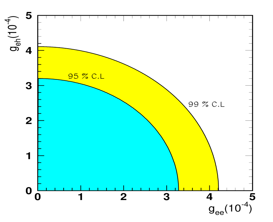
Figure 1: SN 1987A constraint on the majoron-neutrino effective coupling constants in the $g_{ee}-g_{eh}$ plane. Parameters corresponding to the SMA-MSW solution to the solar neutrino problem are assumed.

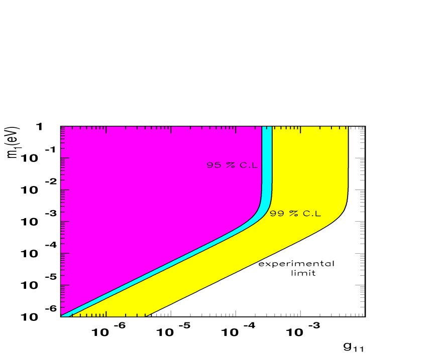
Figure 2: SN 1987A constraint plotted in the $m_{1}-g_{11}$ plane. Parameters corresponding to the LMA-MSW solution to the solar neutrino problem are assumed, $\sin^{2}2\theta=0.6$ and $\Delta_{0}=10^{-5}$ eV².

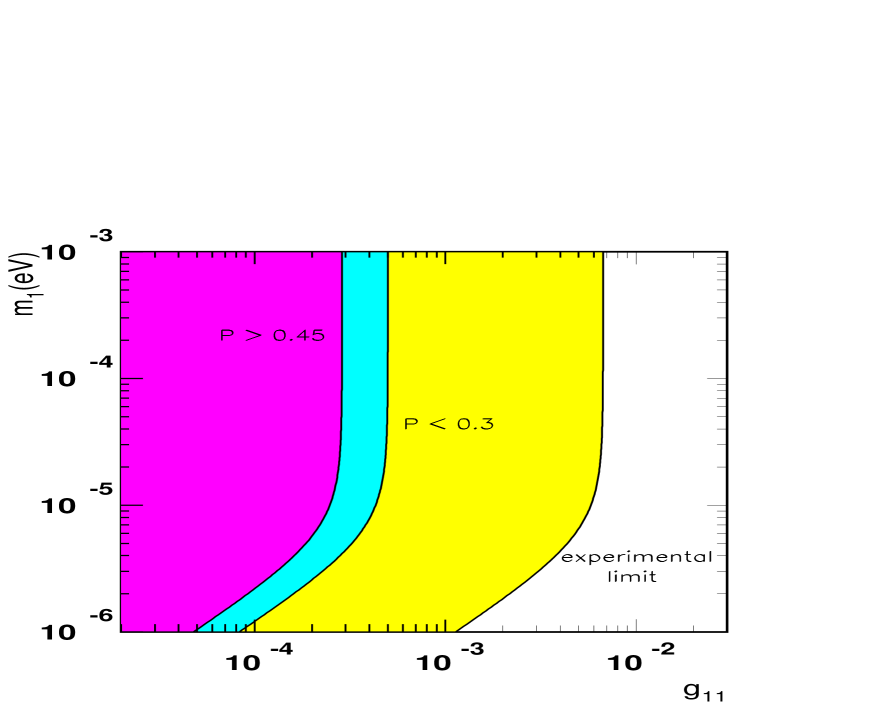
Figure 3: Regions of total transition probability plotted in the $m_{1}-g_{11}$ plane. Here we assume the just–so solution to the solar neutrino problem, $\sin^{2}2\theta=0.9$ and $\Delta_{0}=10^{-10}$ eV² and include both the effects of neutrino decays and oscillation.

Figure 4: Signal expected in Super-Kamiokande due to the reaction $\bar{\nu}_{e}+p\to n+e^{+}$ for a galactic supernova. Here $N_{\nu}$ denotes the number of events for $g_{11}=0$ (solid line) and $g_{11}=10^{-4}$ (dashed line) with $g_{11}=g_{22}=g_{33}$.

Figure 5: Signal expected at SNO due to the reaction $\nu_{h}+D\to\nu_{h}+p+n$ for a galactic supernova. Here $N_{\nu}$ denotes the number of events for the indicated values of $g_{11}$ with $g_{11}=g_{22}=g_{33}$.

References

- [1] Invited talks by T. Kirsten at TAUP 99, Paris, September, 1999 and by Y. Suzuki at XIX Lepton Photon Symposium at Stanford University, August 1999. For a recent overview see also J. Bahcall and R. Davis, “The evolution of neutrino astronomy,” astro-ph/9911486.
- [2] Invited talk by A. Mann at XIX Lepton Photon Symposium at Stanford University, August 1999
- [3] J. Schechter and J.W.F. Valle, Phys. Rev. D22 (1980) 2227.
- [4] L.J. Hall, V.A. Kostelecky and S. Raby, Nucl. Phys. B267 (1986) 415.
- [5] S. Bergmann and A. Kagan, Nucl. Phys. B538 (1999) 368 hep-ph/9803305.
- [6] J.W.F. Valle, Phys. Lett. 131B (1983) 87; G.B. Gelmini and J.W.F. Valle, Phys. Lett. 142B (1984) 181; M.C. Gonzalez-Garcia and J.W.F. Valle, Phys. Lett. B216 (1989) 360; J.C. Romao and J.W.F. Valle, Nucl. Phys. B381 (1992) 87. A.S. Joshipura and J.W.F. Valle, Nucl. Phys. B440 (1995) 647, hep-ph/9410259.
- [7] V. Barger, J.G. Learned, P. Lipari, M. Lusignoli, S. Pakvasa and T.J. Weiler, hep-ph/9907421.
- [8] P.I. Krastev and J.N. Bahcall, hep-ph/9703267.
- [9] M.C. Gonzalez-Garcia et al., Phys. Rev. Lett. 82 (1999) 3202 hep-ph/9809531; N. Fornengo, M.C. Gonzalez-Garcia and J.W.F. Valle, hep-ph/9906539.
- [10] Updated global MSW analyses including the latest 825 day SuperKamiokande data have been given in M.C. Gonzalez-Garcia, P.C. de Holanda, C. Pena-Garay, and J.W.F. Valle, Status of the MSW Solutions of the Solar Neutrino Problem, hep-ph/9906469, to be published in Nucl. Phys. B (1999) and by G.L. Fogli, E. Lisi, D. Montanino and A. Palazzo, hep-ph/9912231.
- [11] Updated vacuum oscillation fits are given in V. Barger and K. Whisnant, Phys. Rev. D59, 093007 (1999); S. Goswami, D. Majumdar and A. Raychaudhuri, hep-ph/9909453.
- [12] M. C. Gonzalez-Garcia, H. Nunokawa, O. L. G. Peres, T. Stanev, J. W. F. Valle, Phys. Rev. D58 (1998) 033004 [hep-ph 9801368]; M.C. Gonzalez-Garcia, H. Nunokawa, O.L. Peres and J.W.F. Valle, Nucl. Phys. B543, 3 (1998), hep-ph/9807305; G.L. Fogli, E. Lisi, D. Montanino and G. Scioscia, Phys. Rev. D55 (1997) 4385; for the most recent update including the 52 kton yr data sample of SuperKamiokande see M.C. Gonzalez-Garcia, hep-ph/9910494, proceedings of the 5th International Workshop “Valencia 99: Particles in Astrophysics and Cosmology”, May 3-8, 1999, Valencia, Spain, ed. V. Berezinsky, G. Raffelt, J. W. F. Valle, Nucl. Phys. Proc. Suppl.
- [13] W.C. Louis [LSND Collaboration], Prog. Part. Nucl. Phys. 40 (1998) 151.
- [14] J.T. Peltoniemi, D. Tommasini and J.W.F. Valle, Phys. Lett. B298 (1993) 383. A. Ioannisian and J.W.F. Valle, hep-ph/9911349. J.T. Peltoniemi and J.W.F. Valle, Nucl. Phys. B406 (1993) 409 hep-ph/9302316. D.O. Caldwell and R.N. Mohapatra, Phys. Rev. D48 (1993) 3259.
- [15] Y. Chikashige, R.N. Mohapatra and R.D. Peccei, Phys. Lett. 98B (1981) 265; G.B. Gelmini and M. Roncadelli, Phys. Lett. 99B (1981) 411.
- [16] J. Schechter and J.W.F. Valle, Phys. Rev. D25 (1982) 774.
- [17] J.W.F. Valle, Prog. Part. Nucl. Phys. 26 (1991) 91.
- [18] E.W. Kolb, D.L. Tubbs and D.A. Dicus, Astrophys J. 255, L57 (1982); D.A. Dicus, E.W. Kolb and D.L. Tubbs, Nucl. Phys. B223, 532 (1983). G.M. Fuller, R. Mayle and J.R. Wilson, Astrophys J. 332, 826 (1988);
- [19] Z.G. Berezhiani and A.Y. Smirnov, Phys. Lett. B220, 279 (1989).
- [20] K. Choi, C.W. Kim, J. Kim and W.P. Lam, Phys. Rev. D37, 3225 (1988); A. Manohar, Phys. Lett. 192B, 217 (1987); J.A. Grifols, E. Masso and S. Peris, Phys. Lett. B215, 593 (1988).
- [21] K. Choi and A. Santamaria, Phys. Rev. D42, 293 (1990).
- [22] T. Bernatowicz et al., Phys. Rev. Lett. 69, 2341 (1992).
- [23] D.I. Britton et al., Phys. Rev. D49, 28 (1994).
- [24] V. Barger, W.Y. Keung and S. Pakvasa, Phys. Rev. D25, 907 (1982).
- [25] L. Wolfenstein, Nucl. Phys. B186 (1981) 147; J.W.F. Valle, Phys. Rev. D27 (1983) 1672; J.W.F. Valle and M. Singer, Phys. Rev. D28 (1983) 540.
- [26] Z.G. Berezhiani and M.I. Vysotsky, Phys. Lett. B199, 281 (1987).
- [27] C. Bemporad [Chooz Collaboration], Nucl. Phys. Proc. Suppl. 77, 159 (1999).
- [28] This simplified form of the lepton mixing matrix was first given in J. Schechter and J.W.F. Valle, Phys. Rev. D21, 309 (1980).
- [29] C. Giunti, C.W. Kim and U.W. Lee, Phys. Rev. D45, 1557 (1992).
- [30] P.D. Mannheim, Phys. Rev. D37, 1935 (1988).
- [31] Z.G. Berezhiani and A. Rossi, Phys. Lett. B336, 439 (1994).
- [32] S.W. Bruenn, Astrophys. J. 340, 955 (1989).
- [33] E. Baron, H.A. Bethe, G.E. Brown, J. Cooperstein, and S. Kahana, Phys. Rev. Lett. 59, 736 (1989).
- [34] S.W. Bruenn, Astrophys. J. Supp. 58, 771 (1985).
- [35] K. Sato and H. Suzuki, Phys. Lett. B196, 267 (1987); H.-T. Janka, in Proc. 5th Ringberg Workshop on Nuclear Astrophysics, Schloß Ringberg 1989.
- [36] B. Jegerlehner, F. Neubig and G. Raffelt, Phys. Rev. D54, 1194 (1996).
- [37] D.A. Dicus, S. Nussinov, P.B. Pal and V.L. Teplitz, Phys. Lett. B218, 84 (1989).
- [38] H.-T. Janka and G. Raffelt, Phys. Rev. D59, 023005 (1999).
- [39] H.-T. Janka, in Proc. Frontier Objects in Astrophysics and Particle Physics, Vulcano 1992, eds. F. Giovaelli and G. Mannocchi.
- [40] We adopt Wilson’s profile as given in H. Nunokawa, J.T. Peltoniemi, A. Rossi and J.W.F. Valle, Phys. Rev. D56, 1704 (1997).
- [41] A.Yu. Smirnov, D.N. Spergel and J.N. Bahcall, Phys. Rev. D49, 1389 (1994).
- [42] A. Burrows, D. Klein and R. Gandhi, Phys. Rev. D45, 3361 (1992).
- [43] J.F. Beacom, preprint hep-ph/9909231 and references therein.
- [44] J.N. Bahcall, P.I. Krastev and E. Lisi, Phys. Rev. C55, 494 (1997).
- [45] S. Ying, W.C. Haxton and E.M. Henley, Phys. Rev. C45, 1982 (1992); K. Kubodera and S. Nozawa, Int. J. Phys. E3, 102 (1994).
- [46] H.-T. Janka and W. Hillebrandt, Astron. Astrophys. 224, 49 (1989).
- [47] P.M. Givanoni, D.C. Ellison and S.W. Bruenn, Astrophys. J. 342, 416 (1989).
- [48] A. Ioannissyan, J.W.F. Valle, Phys. Lett. B332 (1994) 93; B. Bamert, C.P. Burgess, Phys. Lett. B329 (1994) 289; D. Caldwell and R.N. Mohapatra, Phys. Rev. D50 (1994) 3477; D.G. Lee and R.N. Mohapatra, Phys. Lett. B329 (1994) 463; A.S. Joshipura, Z. Phys. C64 (1994) 31.
- [49] V. Barger, S. Pakvasa, T.J. Weiler and K. Whisnant, Phys. Lett. B437, 107 (1998), hep-ph/9806387; S. Davidson and S.F. King, Phys. Lett. B445, 191 (1998).