On the Resummed Hadronic Spectra
of Inclusive $B$ Decays

Abstract

In this paper we investigate the hadronic mass spectra of inclusive $B$ decays. Specifically, we study how an upper cut on the invariant mass spectrum, which is necessary to extract $V_{ub}$, results in the breakdown of the standard perturbative expansion due to the existence of large infrared logs. We first show how the decay rate factorizes at the level of the double differential distribution. Then, we present closed form expressions for the resummed cut rate for the inclusive decays $B\rightarrow X_{s}\,\gamma$ and $B\rightarrow X_{u}\,e\,\nu$ at next-to-leading order in the infrared logs. Using these results, we determine the range of cuts for which resummation is necessary, as well as the range for which the resummed expansion itself breaks down. We also use our results to extract the leading and next to leading infrared log contribution to the two loop differential rate. We find that for the phenomenologically interesting cut values, there is only a small region where the calculation is under control. Furthermore, the size of this region is sensitive to the parameter $\bar{\Lambda}$. We discuss the viability of extracting $V_{ub}$ from the hadronic mass spectrum.

I Introduction

Inclusive $B$ decays are considered fertile ground for precision tests of the standard model. The process $B\to X_{u}\,e\,\nu$ can be used to extract the all important Cabibbo-Kobayashi-Maskawa (CKM) matrix element $V_{ub}$, while $B\to X_{s}\gamma$ decays are important for discovering new physics. However, the utility of experimental measurements of these processes is bounded by our ability to control the theoretical errors. Tremendous effort has gone into determining ways to calculate these rates in a systematic fashion. Indeed, the algorithm for calculating these rates is now part of the theoretical canon [1]. Unfortunately, experimental cuts complicate life for theorists. In particular, these cuts often force us to work near the boundary of the phase space, where the aforementioned canonical techniques break down. Only now are we learning how to retool our calculations to accommodate these highly non-trivial issues.

The complications arise if the cut forces us into a corner of phase space, since the calculation can now depend on a new parameter, $\rho$, which is a measure of the relative size of phase space of interest. When this parameter becomes parametrically small, the systematics of the calculation usually break down; perturbative QCD corrections become enhanced by large logs of the form $\log{\rho}$, while the non-perturbative expansion in $\Lambda/m_{b}$ becomes an expansion in $\Lambda/(\rho\,m_{b})$.

The most relevant cut rate arises in semi-leptonic $B$ decays, where one wishes to measure $V_{ub}$ by eliminating the large background from charmed transitions. To eliminate this background, we have a choice of variables with which to cut. Perhaps the simplest choice is the electron energy, which is the oldest method used for extracting $|V_{ub}|$. Unfortunately, as has been widely discussed in the literature, such extractions are typically model dependent since the rate in this window is sensitive to the Fermi motion of the heavy quark. There is no way to write down a meaningful theoretical error for such extractions. It is only very recently that a model independent method has been proposed, within a well defined systematic scheme [2], that could lead to an extraction with a well defined error.

It is also possible to remove the background from charmed transitions by cutting on the hadronic invariant mass [3]. While this choice presents a greater experimental challenge, it benefits from the fact that, unlike the electron spectrum, most of the $B\rightarrow X_{u}e\nu$ decays are expected to lie within the region $s_{H}<M_{D}^{2}$. Furthermore, it is believed that even though both the invariant mass region $s_{H}<M_{D}^{2}$ and electron energy regions $M_{B}/2>E_{e}>(M_{B}^{2}-M_{D}^{2})/(2M_{B})$ receive contributions from hadronic final states with invariant mass up to $M_{D}$, the cut mass spectrum will be less sensitive to local duality violations. This belief rests on the fact that the contribution of large mass states is kinematically suppressed for the electron energy spectrum in the region of interest.

The goal of this paper is to study the viability of extracting $V_{ub}$ from the invariant mass spectrum. In particular, we are interested in studying the breakdown of the perturbative expansion for the cut rate, and whether or not a reorganized expansion can be used reliably.

Building upon the work of Korchemsky and Sterman [4], we begin by discussing how the doubly differential decay rate factorizes in moment space. We then use the recent results of [2] to calculate a closed form expression for the inverse Mellin transform at next-to-leading logarithmic (NLL) order. The result for the resummed rate is presented in terms of the partonic as well as hadronic invariant mass. This result is used to extract a piece of the two loop rate, the size of which can be compared to the Brodsky-Lepage-Mackenzie (BLM) two loop correction. We then determine the region of invariant mass where resummation is necessary as well as the region where the reorganized expansion breaks down. We conclude with a brief discussion of the phenomenology, saving a complete discussion, including the effects of Fermi motion, for a later publication[5].

II Factorization in Hadronic Variables

The problem of summing large threshold logarithms in perturbative expansions, which arise due to incomplete KLN cancellation of the IR sensitivity at the edge of phase space, has been addressed for various processes [6]. The technique relies on factorization, which allows for resummations via a renormalization group equation. The factorization in $B$ decays has been previously discussed in leptonic variables in [4, 7]. Here we review the arguments that are germane to our discussion of factorization in terms of hadronic variables.

Consider the inclusive semi-leptonic decay of the $b$ quark into a lepton pair with momenta $q=(p_{e}+p_{\nu})$ and a hadronic jet of momenta $p_{h}$. It is convenient to define the following partonic kinematic variables in the rest frame of the $B$ meson $v=(1,\vec{0})$,

$$\hat{s}_{0}=\frac{p_{h}^{2}}{m_{b}^{2}},\quad h=\frac{2v\cdot p_{h}}{m_{b}},\quad x=\frac{2v\cdot p_{e}}{m_{b}},$$ (1)

with phase space boundaries

$$0\leq\hat{s}_{0}\leq 1,\quad 2\sqrt{\hat{s}_{0}}\leq h\leq 1+\hat{s}_{0},\quad 1-\frac{h}{2}-\frac{1}{2}\sqrt{h^{2}-4\hat{s}_{0}}\leq x\leq 1-\frac{h}{2}+\frac{1}{2}\sqrt{h^{2}-4\hat{s}_{0}}.$$ (2)

In addition, it is customary to define the leptonic variables

$$y_{0}=\frac{2v\cdot q}{m_{b}},\quad y=\frac{q^{2}}{m_{b}^{2}}.$$ (3)

In terms of the leptonic variables, $\hat{s}_{0}=(1-y_{0}+y)$ and $h=2-y_{0}$, one can see that in the endpoint region of the electron energy spectrum when $x\to 1$ with $y<1$, the invariant mass of the jet approaches zero with its energy held fixed. In addition, the jet hadronizes at a much later time in the rest frame of the $B$ meson, due to the time dilation. Factorization exploits this and separates the particular differential rate under consideration into subprocesses with disparate scales. This factorization fails when the jet energy vanishes in the dangerous region $y\to x\to 1$. However, this problematic region of phase space is suppressed because the rate to produce soft massless fermions vanishes at tree level.

The infrared sensitive regions, which give rise to the large logarithms, can be determined by constructing a reduced diagram, as shown in Fig. 1. According the Coleman-Norton theorem [8], a diagram at the infrared singular point must describe a physically realizable process after contracting all off-shell lines to a point. In the figure, $S$ denotes a soft blob which interacts with the jet and the $b$ quark via soft lines. $J$ denotes the hadronic jet and $H$ the hard scattering amplitude. Thus, the reduced diagram in Fig. 1 is simply a visualization of factorization. An important consequence of this factorization is that the soft function $S$ is universal. Moreover, it has been shown [4] that the soft function $S$ contains the non-perturbative structure function introduced in Ref. [9]. It is this universality that will eventually allow us to eliminate the dependence on unknown non-perturbative hadronic dynamics[2, 5].

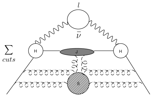
FIG. 1.: Reduced diagram for inclusive B decays.

From the above discussions one can see that in terms of the variables introduced earlier, factorization holds when $\hat{s}_{0}\sim 0$ and $h\sim 1$, or equivalently $1\gg\hat{s}_{0}/h$. The typical momenta flowing through the hard subprocesses are ${\cal O}(m_{b})$. Thus, $H$ does not contain any large threshold logarithms and has a well-defined perturbative expansion in $\alpha_{s}(m_{b})$. The soft function $S$ contains typical momentum $k$, with $k^{+}\sim k^{-}\sim k_{\perp}={\cal O}(m_{b}\,\hat{s}_{0}/h)$. By soft we mean soft compared to $m_{b}$, but still larger than $\Lambda_{\rm QCD}$. For an energetic $u$ quark moving in the ’$-$’ direction, the jet subprocess has typical momenta $p$ such that $p^{-}\gg p^{+},p_{\perp}$ with $p^{+}={\cal O}(m_{b}\,\hat{s}_{0}/h)$, $p^{2}_{\perp}={\cal O}(m_{b}^{2}\,\hat{s}_{0}/h)$, and $p^{-}={\cal O}(m_{b})$. In order to delineate between momentum regimes, a factorization scale $\mu$ is introduced. The fact that the process is independent of the factorization scale $\mu$ is utilized to sum the large threshold logarithms in the soft and jet functions. The reduced diagram for the inclusive radiative decays $B\to X_{s}\gamma$ is exactly the same as above if we replace the lepton pair with a photon and ignore the strange quark mass.

In terms of $\hat{s}_{0}$ and $h$, the triply differential rate, which factorizes into hard, jet and soft subprocesses[4], may be written as

$$\frac{1}{\Gamma_{0}}\frac{d^{3}\Gamma}{d\hat{s}_{0}\,dh\,dx}=$$ (4)

$$\quad\quad 12\,(2-h-x)(x+h-1-\hat{s}_{0})\int_{\xi}^{M_{B}/m_{b}}dz\,S(z)\,m_{b}^{2}\,J[m_{b}^{2}\;h(z-\xi),\mu]\,H(m_{b}\,h/\mu),$$ (5)

$$\phantom{\frac{d^{3}\Gamma}{d\hat{s}_{0}\,dh\,dx}}\Gamma_{0}=\frac{G_{F}^{2}}{192\pi^{3}}|V_{ub}|^{2}m_{b}^{5},$$ (6)

where $\xi=1-\hat{s}_{0}/h$ is analogous to the Bjorken scaling variable in deep inelastic scattering. $z=1+k_{+}/m_{b}$, where $k_{+}$ is the heavy quark light cone residual momentum. $S(z)$ essentially describes the probability for the $b$ quark to carry light cone momentum fraction $z$ and allows for a leakage past the partonic endpoint, as can be seen explicitly in the upper limit of $z$. A similar factorized expression holds for the inclusive radiative decays near the endpoint,

$$\frac{1}{\Gamma_{0}^{\gamma}}\frac{d\Gamma^{\gamma}}{d\hat{s}_{0}} = \int_{1-\hat{s}_{0}}^{M_{B}/m_{b}}dz\;S(z)\,m_{b}^{2}J[m_{b}^{2}(z-1+\hat{s}_{0}),\mu^{2}]\,H(m_{b}/\mu),$$ (7)

$$\Gamma_{0}^{\gamma} = \frac{G_{F}^{2}}{32\pi^{4}}|V_{ts}^{*}V_{tb}|^{2}\,\alpha\;C_{7}^{2}\,m_{b}^{5}.$$ (8)

For the inclusive semi-leptonic decays, the integration over $x$ can be done in the endpoint region and the resulting doubly differential rate is

$$\frac{1}{\Gamma_{0}}\frac{d^{2}\Gamma}{d\hat{s}_{0}\,dh}=2h^{2}(3-2h)\int_{\xi}^{M_{B}/m_{b}}dz\,S(z)\,m_{b}^{2}\,J[m_{b}^{2}\,h(z-\xi),\mu]\,H(m_{b}\,h/\mu)+{\cal O}(\hat{s}_{0}).$$ (9)

This is where the factorization in the invariant mass spectrum is simpler than in the electron energy spectrum. In the latter case, none of the integrals in the triply differential rate can be done trivially and one has to take an extra derivative with respect to $x$ to arrive at an expression similar to Eq. (9). An interesting consequence of factorization is that it connects the electron energy spectrum in the region $x\to 1$ with the invariant mass spectrum, in the region $\hat{s}_{0}\to 0$,

$$\left.\frac{d\Gamma}{d\hat{s}_{0}}\right|_{\hat{s}_{0}\to 1-x}=-\frac{1}{2}\;\frac{d}{dx}\,\frac{d\Gamma}{dx},$$ (10)

which can be verified explicitly at the one loop level using the corresponding expressions in Ref. [10].

III The Perturbative Resummation

At one loop level the differential rates are [10, 11]

$$\frac{1}{\Gamma_{0}}\,\frac{d^{2}\Gamma}{d\hat{s}_{0}\,dh} = 2h^{2}\,(3-2h)\left[\delta(\hat{s}_{0})+\frac{C_{F}\alpha_{s}}{4\pi}E_{1}(h,\hat{s}_{0})\right]+\frac{C_{F}\alpha_{s}}{4\pi}E_{2}(h,\hat{s}_{0}),$$ (11)

$$\frac{1}{\Gamma_{0}^{\gamma}}\,\frac{d\Gamma^{\gamma}}{d\hat{s}_{0}} = \delta(\hat{s}_{0})\left[1-\frac{C_{F}\alpha_{s}}{4\pi}\left(13+\frac{4}{3}\pi^{2}\right)\right]$$ (13)

$$+\frac{C_{F}\alpha_{s}}{4\pi}\left[6+3\hat{s}_{0}-2\hat{s}_{0}^{2}-2(2-\hat{s}_{0})\log\hat{s}_{0}-\left(\frac{7}{\hat{s}_{0}}+4\,\frac{\log\hat{s}_{0}}{\hat{s}_{0}}\right)_{+}\right],$$

where

$$E_{1}(h,\hat{s}_{0}) = -\delta(\hat{s}_{0})\left[8\log^{2}(h)-10\log h+\frac{2\log h}{1-h}+4\,{\rm Li}_{2}(1-h)+5+\frac{4}{3}\pi^{2}\right]$$ (15)

$$-4\left(\frac{\log\hat{s}_{0}}{\hat{s}_{0}}\right)_{+}+(8\log h-7)\left(\frac{1}{\hat{s}_{0}}\right)_{+}+\frac{1}{\hat{s}_{0}}\left[8\log\left(\frac{1+t}{2}\right)+7(1-t)\right],$$

$$E_{2}(h,\hat{s}_{0}) = \delta(\hat{s}_{0})\,\frac{4h^{3}\log h}{1-h}-4\left[2h(3-4h)-3(1-2h)\hat{s}_{0}-2\hat{s}_{0}^{2}\right]\log\left(\frac{1+t}{1-t}\right)$$ (17)

$$+\,4\,h\,t\,(10-15h+8\hat{s}_{0}),$$

and $t=\sqrt{1-4\hat{s}_{0}/h^{2}}$. We also adopt the following definition for the ’+’ distributions

$$\left(\frac{\log^{n}(\hat{s}_{0})}{\hat{s}_{0}}\right)_{+}=\lim_{\epsilon\to 0}\left[\theta(\hat{s}_{0}-\epsilon)\frac{\log^{n}(\hat{s}_{0})}{\hat{s}_{0}}+\delta(\hat{s}_{0})\,\frac{\log^{n+1}(\epsilon)}{n+1}\right].$$ (18)

This definition is such that

$$\int_{0}^{\rho}\,d\hat{s}_{0}\,F(\hat{s}_{0})\left(\frac{\log^{n}(\hat{s}_{0})}{\hat{s}_{0}}\right)_{+}=F(0)\,\frac{\log^{n+1}(\rho)}{n+1}\,+\,\int_{0}^{\rho}\,d\hat{s}_{0}\,\left[F(\hat{s}_{0})-F(0)\right]\,\frac{\log^{n}(\hat{s}_{0})}{\hat{s}_{0}}.$$ (19)

Note that if the parameter $\rho$ becomes parametrically small, the first term on the right hand side of Eq. (19) will give large logarithms thereby spoiling the systematics of the perturbative expansions, while the second term must be regular as $\rho\to 0$. To perform the resummation we go into the moment space where the amplitudes factorize completely. In the case of inclusive semi-leptonic decays, it is convenient to define a new variable $\lambda=\hat{s}_{0}/h$ with kinematic range

$$0\leq h\leq 1\;;\quad 0\leq\lambda\leq\frac{h}{4},$$ (20)

$$1\leq h\leq 2\;;\quad 1-\frac{1}{h}\leq\lambda\leq\frac{h}{4}.$$ (21)

The region with $h\geq 1$ is populated with real gluon emissions only, whereas the region with $h\leq 1$ has both real and virtual gluon corrections. In the relevant region $h\to 1$ and $\lambda\to 0$ the contributions from real and virtual gluon emissions combine to give terms which are ’+’ distributions, which upon integrating up to a cut, lead to the large logs we wish to resum.

To proceed, we take the $N$th moment with respect to $\xi=1-\lambda$ in the large $N$ limit. In the region $\hat{s}_{0}\sim 0$ and $z\sim\xi\sim 1$, one can replace $J[m_{b}^{2}\,h(z-\xi)]$ in Eq. (9) with $J[m_{b}^{2}\,h(1-\xi/z)]$. This replacement is permissible to the order we are working. We then obtain

$$M_{N} = \int_{0}^{1}d\lambda\;(1-\lambda)^{N-1}\frac{1}{\Gamma_{0}}\,\frac{d^{2}\Gamma}{d\lambda\,dh}$$ (22)

$$= 2h^{2}(3-2h)\,S_{N}\,J_{N}(m_{b}^{2}\,h/\mu^{2})\,H(m_{b}\,/\mu)+{\cal O}(1/N),$$ (23)

$$J_{N}(m_{b}^{2}/\mu^{2}) = m_{b}^{2}\int_{0}^{1}dy\,y^{N-1}J[m_{b}^{2}(1-y),\mu],$$ (24)

$$S_{N} = \int_{0}^{M_{B}/m_{b}}dz\;z^{N}S(z).$$ (25)

The soft moment $S_{N}$ further decomposes into a perturbative soft piece, which accounts for soft gluon radiation and a non-perturbative piece which incorporates bound state dynamics and serves as the boundary condition for the renormalization group equation [4].

$$S(z) = \int_{z}^{M_{b}/m_{b}}\frac{dy}{y}f[m_{b}(1-y)]\,\sigma(z/y),$$ (26)

$$S_{N} = f_{N}\,\sigma_{N},$$ (27)

where $f(y)=\langle B(v)|\,\bar{b}_{v}\,\delta(y-iD_{+})\,b_{v}\,|B(v)\rangle$ is the non-perturbative structure function defined in Ref. [9]. A similar expression holds for the inclusive radiative decays $B\to X_{s}\gamma$

$$M_{N}^{\gamma} = \int_{0}^{1}d\hat{s}_{0}\,(1-\hat{s}_{0})^{N-1}\frac{1}{\Gamma_{0}^{\gamma}}\,\frac{d\Gamma^{\gamma}}{d\hat{s}_{0}}$$ (28)

$$= f_{N}\,\sigma_{N}\,J_{N}\,H^{\gamma}+{\cal O}(1/N),$$ (29)

Subsequently, we will ignore the non-perturbative structure function $f(y)$ and concentrate on the perturbative resummations.

It merits emphasizing that the large $N$ asymptotics of the moments corresponds to the behavior of the spectra in the region $\hat{s}_{0}\sim\lambda\sim 0$. Taking the large $N$ limit also enables us to extend the integration limit of $\lambda$ in Eq. (22) up to $1$, despite the fact that the kinematic range of $\lambda$ never goes up to $1$. In this limit the contribution from the region $\lambda\sim 1$ is power suppressed.

Comparing Eq. (22) with the corresponding expression for the electron energy spectrum in Ref. [4], one sees that the moments $\sigma_{N}$ and $J_{N}$ are identical with those in the electron energy spectrum, with change of variables $x\to 1-\lambda$ and $2-y_{0}\to h$. A similar identification for the resummed radiative decays, Eq. (28), can be made with the change of variables $x\to 1-\hat{s}_{0}$. In moment space the soft and jet functions [12] have been calculated to NLL order and are given by

$$\sigma_{N}\,J_{N} = \exp[\,\log(N)\,g_{1}(\chi)+g_{2}(\chi)]$$ (30)

$$\sigma_{N}\,J_{N}^{\gamma} = \exp[\,\log(N)\,g_{1}(\chi)+g_{2}^{\gamma}(\chi)],$$ (31)

where $\chi=\alpha_{s}(m_{b}^{2})\beta_{0}\log N$, and $g_{1}$ and $g_{2}$ are given explicitly as [7]

$$g_{1}(\chi) = -\frac{2}{3\pi\beta_{0}\chi}[(1-2\chi)\log(1-2\chi)-2(1-\chi)\log(1-\chi)],$$ (32)

$$g_{2}(\chi) = g_{2}^{\gamma}(\chi)+g_{sl}(\chi,h),$$ (33)

$$g_{2}^{\gamma}(\chi) = -\frac{k}{3\pi^{2}\beta_{0}^{2}}\left[\,2\log(1-\chi)-\log(1-2\chi)\right]-\frac{2\beta_{1}}{3\pi\beta_{0}^{3}}\left[\log(1-2\chi)-2\log(1-\chi)\frac{}{}\right.$$ (36)

$$+\left.\,\frac{1}{2}\log^{2}(1-2\chi)-\log^{2}(1-\chi)\right]-\frac{1}{\pi\beta_{0}}\log(1-\chi)-\frac{2}{3\pi\beta_{0}}\log(1-2\chi)$$

$$+\,\frac{4\gamma_{E}}{3\pi\beta_{0}}\left[\log(1-2\chi)-\log(1-\chi)\right],$$

$$g_{sl}(\chi,h) = \frac{4}{3\pi\beta_{0}}\log(h)\log(1-\chi).$$ (37)

In the above, $\beta_{0}=(11\,C_{A}-2\,N_{f})/(12\pi)$, $\beta_{1}=(17\,C_{A}^{2}-5\,C_{A}\,N_{f}-3\,C_{F}\,N_{f})/(24\pi^{2})$, $k=C_{A}\,(67/18-\pi^{2}/6)-10\,T_{R}\,N_{f}/9$, and $\gamma_{E}=0.577216...$ is the Euler-Mascheroni constant. In our case, $C_{A}=3$, $C_{F}=4/3$, and $T_{R}=1/2$. To get back the physical spectra from the moment space, the inverse Mellin transform has to be evaluated at NLL accuracy as well. To this end, we apply the identity derived in the Appendix of Ref. [2]

$$\frac{1}{2\pi i}\;\int_{C-i\infty}^{C+i\infty}\,dN\,x^{-N}\,e^{\log(N)\,F_{1}[\alpha_{s}\log N]+F_{2}[\alpha_{s}\log N]}$$ (38)

$$\phantom{\frac{1}{2\pi i}\;\int_{C-i\infty}^{C+i\infty}}=-x\frac{d}{dx}\;\left\{\theta(1-x)\frac{e^{l\>F_{1}(\alpha_{s}l)+F_{2}(\alpha_{s}l)}}{\Gamma\left[1-F_{1}(\alpha_{s}l)-\alpha_{s}l\,F_{1}^{\prime}(\alpha_{s}l)\right]}\times\left[1+{\cal F}(\alpha_{s},l)\right]\right\},$$ (39)

where $l=-\log(-\log x)\approx-\log(1-x)$, and

$${\cal F}(\alpha_{s},l)=\sum_{k=1}^{\infty}\alpha_{s}^{k}\,\sum_{j=0}^{k-1}f_{kj}\,l^{j}$$ (40)

represents next-to-next-to-leading log contributions. Changing variables from $\lambda$ back to $\hat{s}_{0}/h$, we obtain

$$\frac{1}{\Gamma_{0}}\,\frac{d^{2}\Gamma}{d\hat{s}_{0}\,dh} = 2h^{2}(3-2h)\,H(h)$$ (42)

$$\times\frac{d}{d\hat{s}_{0}}\left\{\,\theta\left(\frac{\hat{s}_{0}}{h}-\eta\right)\,\frac{e^{l\>g_{1}(\alpha_{s}\beta_{0}\,l)+g_{2}(\alpha_{s}\beta_{0}\,l)}}{\Gamma\left[1-g_{1}(\alpha_{s}\beta_{0}\,l)-\alpha_{s}\beta_{0}\,l\,g_{1}^{\prime}(\alpha_{s}\beta_{0}\,l)\right]}\right\},$$

$$\frac{1}{\Gamma_{0}^{\gamma}}\,\frac{d\Gamma^{\gamma}}{d\hat{s}_{0}} = H^{\gamma}\,\frac{d}{d\hat{s}_{0}}\left\{\,\theta(\hat{s}_{0}-\eta)\,\frac{e^{l\>g_{1}(\alpha_{s}\beta_{0}\,l^{\gamma})+g_{2}^{\gamma}(\alpha_{s}\beta_{0}\,l^{\gamma})}}{\Gamma\left[1-g_{1}(\alpha_{s}\beta_{0}\,l^{\gamma})-\alpha_{s}\beta_{0}\,l^{\gamma}\,g_{1}^{\prime}(\alpha_{s}\beta_{0}\,l^{\gamma})\right]}\right\},$$ (43)

where $l=-\log\left(-\log(1-\lambda)\right)\approx-\log(\hat{s}_{0}/h)$, and $l^{\gamma}=-\log\left(-\log(1-\hat{s}_{0})\right)\approx-\log(\hat{s}_{0})$. The $\theta$-functions define the differential rates in a distribution sense, as $\eta\to 0$, and turn the singular terms into the ’$+$’ distributions, as can be seen explicitly by expanding in power series of $\log\hat{s}_{0}$ and using the definition Eq. (18).

The hard parts can be obtained through the one loop results Eq. (11) and Eq. (13)

$$H(h) = 1-\frac{2\alpha_{s}}{3\pi}\left[4\log^{2}(h)-5\log h+\frac{3\log h}{3-2h}+2{\rm Li}_{2}(1-h)+\frac{5}{2}+\frac{2\pi^{2}}{3}\right]$$ (44)

$$H^{\gamma} = 1-\frac{2\alpha_{s}}{3\pi}\left(\frac{13}{2}+\frac{2\pi^{2}}{3}\right).$$ (45)

Eq. (42) and Eq. (43) reproduce the dominate contribution at one loop level in the limit $\lambda\to 0$ and $\hat{s}_{0}\to 0$, respectively, and include the infinite set of terms of the form $\alpha_{s}^{n}\log^{n+1}(\hat{s}_{0})$ and $\alpha_{s}^{n}\log^{n}(\hat{s}_{0})$ in the Sudakov exponent for both semi-leptonic and radiative decays.

IV The Integrated Cut Invariant Mass Spectrum

As previously mentioned, it has been proposed that we measure the modulus of the CKM matrix element $V_{ub}$ from inclusive decays by making a cut on the hadronic invariant mass below $M_{D}^{2}$. This cut eliminates the overwhelming background from bottom to charm transitions. While it is the hadronic invariant mass which is of interest, we shall first consider the cut partonic invariant mass, as it will be relevant to our conclusions.

The use of an upper cut $c_{0}$ on the partonic invariant mass introduces large logs of the form $\alpha_{s}\log^{2}(c_{0})$. As $c_{0}$ approaches zero, the logs become parametrically large and need to be resummed. Using the resummation formulas in the previous section, it is simple to generate an expression for the resummed cut rate, since our expression can be written as a total derivative with respect to $\hat{s}_{0}$. The cut rate may be written as

$$\frac{1}{\Gamma_{0}}\,\Gamma(c_{0})=\int_{0}^{1}~{}dh\;2h^{2}(3-2h)\left[\xi\left(\frac{c_{0}}{h}\right)-\xi_{\alpha_{s}}\left(\frac{c_{0}}{h}\right)\right]+\int_{0}^{c_{0}}d\hat{s}_{0}\,\int^{1+\hat{s}_{0}}_{2\sqrt{\hat{s}_{0}}}dh\;\gamma_{\alpha_{s}}(h,\hat{s}_{0}),$$ (46)

where

$$\xi(c_{0}/h)=\left.\frac{e^{l\>g_{1}(\alpha_{s}\beta_{0}\,l)+g_{2}(\alpha_{s}\beta_{0}\,l)}}{\Gamma\left[1-g_{1}(\alpha_{s}\beta_{0}\,l)-\alpha_{s}\beta_{0}\,l\,g_{1}^{\prime}(\alpha_{s}\beta_{0}\,l)\right]}\right|_{l=-\log(c_{0}/h)},$$ (47)

and $\gamma_{\alpha_{s}}(h,\hat{s}_{0})$ is simply the one loop rate defined in Eq. (11). $\xi_{\alpha_{s}}$ stands for terms up to ${\cal O}(\alpha_{s})$ when expanding $\xi$ in power series of $\alpha_{s}$. We subtracted it from $\xi$ in order to ensure that we correctly reproduce the one loop result at order $\alpha_{s}$. From Eq. (46) one can see that the large logs arise when $\hat{s}_{0}$ approaches zero, which is not only the lower kinematic limit for $\hat{s}_{0}$, but also the phase space boundary for virtual and real gluon emissions.

The perturbative expansion has been reorganized into an expansion in the exponent. The systematics of this expansion have been discussed at length in [2, 13]. Here we just recall that we may test the convergence of the reorganized expansion by comparing the NLL resummed result with the leading-logarithm (LL) resummed result. Fig. 2 shows the cut rate as a function of $c_{0}$. In this figure we show the one loop cut rate as well as the resummed cut rate with and without NLL corrections. We see that for $0.1<c_{0}<0.2$ the resummation becomes necessary, while for $c_{0}<0.1$ the NLL dominates the LL, so that we can no longer trust our results. Indeed, this breakdown occurs well before we reach the Landau pole at $\hat{s}_{p}=e^{-1/(2\alpha_{s}\beta_{0})}\approx 0.028$.

FIG. 2.: The rate as a function of the partonic cut. The dotted line is the one loop result, the dashed line is the LL result, while the solid line is the NLL log result. The difference between the one loop and resummed results at large $c_{0}$ is due to two loop corrections introduced in the resummation. We use $\alpha_{s}(m_{b})=0.21$.

We now expand this result to pick out the leading and next to leading infrared log contribution to the two loop differential rate. This contribution is given by

$$\frac{1}{\Gamma_{0}}\left.\frac{d\Gamma}{d\hat{s}_{0}dh}\right|_{{\cal O}(\alpha_{s}^{2})}=2h^{2}(3-2h)\,\frac{\alpha_{s}^{2}}{3\pi^{2}}\,\left[\frac{8}{3}\left(\frac{\log^{3}(\hat{s}_{0})}{\hat{s}_{0}}\right)_{+}+(14-6\pi\beta_{0})\left(\frac{\log^{2}(\hat{s}_{0})}{\hat{s}_{0}}\right)_{+}\right]$$ (48)

As expected, we see that the most singular contribution at ${\cal O}(\alpha_{s}^{2})$ doesn’t have any terms proportional to $\beta_{0}$. It may be the case that, in this particular region of phase space the infrared logs terms may dominate over the BLM terms. Such a conclusion was reached in [2, 13] for the two loop contribution to lepton and photon spectra in semi-leptonic and radiative decays, respectively. Naturally , this does not preclude the possibility that there exist a cancellation with other uncalculated terms, such that the $\alpha_{s}^{2}\beta_{0}$ still dominate.

Let us now consider the physical case, where we are interested in placing an upper cut on the hadronic invariant mass. The hadronic invariant mass may be written as

$$\hat{s}_{H} = \frac{s_{H}}{m_{b}^{2}}=\hat{s}_{0}+\epsilon h+\epsilon^{2},$$ (49)

$$\epsilon = \frac{\bar{\Lambda}}{m_{b}},$$ (50)

where $\bar{\Lambda}$ is the mass difference $M_{B}-m_{b}$ in the infinite $b$ quark mass limit, which is a measure of binding energy for the $b$ quark inside the $B$ meson. Thus, given a cut on $\hat{s}_{H}$, $c$, we may translate this into an $h$ dependent cut on $\hat{s}_{0}$. After changing the order of integration we find that the cut rate may be written as

$$\frac{1}{\Gamma_{0}}\Gamma(c)=\int^{\frac{c-\epsilon(1+\epsilon)}{1+\epsilon}}_{0}d\hat{s}_{0}\int_{2\sqrt{\hat{s}_{0}}}^{1+\hat{s}_{0}}dh\left(\frac{d\Gamma}{d\hat{s}_{0}dh}\right)+\int_{\frac{c-\epsilon(1+\epsilon)}{1+\epsilon}}^{(\sqrt{c}-\epsilon)^{2}}d\hat{s}_{0}\int^{\frac{c-\hat{s}_{0}-\epsilon^{2}}{\epsilon}}_{2\sqrt{\hat{s}_{0}}}dh\left(\frac{d\Gamma}{d\hat{s}_{0}dh}\right),$$ (51)

if $c>\epsilon(1+\epsilon)$, whereas if $c<\epsilon(1+\epsilon)$ then

$$\frac{1}{\Gamma_{0}}\Gamma(c)=\int^{(\sqrt{c}-\epsilon)^{2}}_{0}d\hat{s}_{0}\int_{2\sqrt{\hat{s}_{0}}}^{\frac{c-\hat{s}_{0}-\epsilon^{2}}{\epsilon}}dh\left(\frac{d\Gamma}{d\hat{s}_{0}dh}\right).$$ (52)

This situation is different from the partonic invariant mass spectrum. In the present case, the lower kinematic limit of $\hat{s}_{H}$ is $\epsilon^{2}$, while the phase space boundary for virtual and real gluon emissions has been moved to $\rho_{\epsilon}=\epsilon(1+\epsilon)$, above which only real gluon emissions contribute. Hence there could potentially be two kinds of parametrically large logarithms $\log(c-\epsilon^{2})$ and $\log(c-\rho_{\epsilon})$ appearing. However, as can be seen from Eq. (49), $\hat{s}_{H}\to\epsilon^{2}$ corresponds to vanishing $\hat{s}_{0}$ and $h$, which is the dangerous region where the infra-red factorization fails and is kinematically suppressed by the tree level rate. More explicitly, $\log(c-\epsilon^{2})$ will be killed by the pre-factor $2(c-\epsilon^{2})^{2}$ so that the rate vanishes as $c\to\epsilon^{2}$. The only important parametrically large logarithms are those resulting from the incomplete cancellation between virtual and real corrections at the phase space boundary $\rho_{\epsilon}$. From this argument it would seem that we only need to resum logs of the form $\log(c-\rho_{\epsilon})$. However, in this particular case, the distance from $\rho_{\epsilon}$ to $\epsilon^{2}$ is only $\epsilon$, which is expected to be a numerically small quantity at around $0.08$. If the experimental cut $c$ lies below $\rho_{\epsilon}$, the partially integrated rate could still be sensitive to $\log(c-\epsilon^{2})$ due to the smallness of $\epsilon$. We thus chose to resum all logs of the form $\log(c-\epsilon^{2})$ as well. Fortunately, since we have the resummed rate at the doubly differential level, this is not a problem. The resummed rate with hadronic mass cut $c>\rho_{\epsilon}$ is given by

$$\frac{1}{\Gamma_{0}}\Gamma(c)_{>}= \int_{0}^{1}~{}dh\,2h^{2}(3-2h)\,\left\{\xi\left[\frac{c-\rho_{\epsilon}}{h(1+\epsilon)}\right]-\xi_{\alpha_{s}}\left[\frac{c-\rho_{\epsilon}}{h(1+\epsilon)}\right]\right\}$$ (53)

$$+ \int_{\frac{c-\rho_{\epsilon}}{1+\epsilon}}^{(\sqrt{c}-\epsilon)^{2}}d\hat{s}_{0}\int_{2\sqrt{\hat{s}_{0}}}^{\frac{c-\hat{s}_{0}-\epsilon^{2}}{\epsilon}}dh\,2h^{2}(3-2h)\,\left[\xi^{\prime}(\hat{s}_{0}/h)-\xi^{\prime}_{\alpha_{s}}(\hat{s}_{0}/h)\right]$$ (54)

$$+ \int_{0}^{\frac{c-\rho_{\epsilon}}{1+\epsilon}}d\hat{s}_{0}\int_{2\sqrt{\hat{s}_{0}}}^{1+\hat{s}_{0}}dh\;\gamma_{\alpha_{s}}(h,\hat{s}_{0})+\int_{\frac{c-\rho_{\epsilon}}{1+\epsilon}}^{(\sqrt{c}-\epsilon)^{2}}d\hat{s}_{0}\int_{2\sqrt{\hat{s}_{0}}}^{\frac{c-\hat{s}_{0}-\epsilon^{2}}{\epsilon}}dh\;\gamma_{\alpha_{s}}(h,\hat{s}_{0}),$$ (55)

where

$$\xi^{\prime}(\hat{s}_{0}/h)=\frac{d}{d\hat{s}_{0}}\xi(\hat{s}_{0}/h).$$ (56)

While the resummed rate with hadronic mass cut $c<\rho_{\epsilon}$ is given by

$$\frac{1}{\Gamma_{0}}\Gamma(c)_{<}= \int_{0}^{\frac{c-\epsilon^{2}}{\epsilon}}dh\;2h^{2}(3-2h)\,\left\{\xi\left[\frac{(\sqrt{c}-\epsilon)^{2}}{h}\right]-\xi_{\alpha_{s}}\left[\frac{(\sqrt{c}-\epsilon)^{2}}{h}\right]\right\}$$ (57)

$$+ \int_{0}^{\left(\sqrt{c}-\epsilon\right)^{2}}d\hat{s}_{0}\int_{2\sqrt{\hat{s}_{0}}}^{1+\hat{s}_{0}}\,\gamma_{\alpha_{s}}(h,\hat{s}_{0}).$$ (58)

Analytic expressions for the partially integrated rate at one loop level, last lines in Eq. (53) and Eq. (57), can be found in Ref. [10].

FIG. 3.: The rate with a hadronic cut. The dotted line is the one loop result, the dashed line is the LL resummed result, while the solid line is the NLL resummed result. For $\bar{\Lambda}=0.39\,{\rm GeV}$, we have $\rho_{\epsilon}=0.0861$. In the region above $\rho_{\epsilon}$, we run into Landau pole at $c_{p}=0.1159$ and interpolate in the small region between $\rho_{\epsilon}$ and $c_{p}$.

V Results and Conclusions

In Fig. 3 we show the one loop, LL resummed (including $g_{1}$ only) and NLL resummed (including $g_{1}$ and $g_{2}$) results for $\bar{\Lambda}=0.39\,\mbox{GeV}$. We see the for $c\leq 0.18$, the next to leading order approximation breaks down, as the next to leading order piece becomes just as large as the leading order piece. Notice that when $c\simeq 0.18$, the effective cut on the partonic invariant mass is $c_{0}\simeq 0.09$, which from Fig. 2 we see is consistent with the breakdown of the resummed expansion. This is contrast with the result that an energy cut of $2.1{\rm\ GeV}$, on the rate for $B\rightarrow X_{s}\gamma$ does not necessitate resummation, as the argument of the logs in the case of the radiative decay is about $0.12$.

It is clear from Fig. 3 that resummation shifts the whole spectrum toward the high invariant mass region such that the number of events which lie below the cut $c$ is decreased. This occurs because the high invariant mass region with $\hat{s}_{H}>\rho_{\epsilon}$ is populated with real gluon emissions only.

FIG. 4.: The cut rate for several different values of $\bar{\Lambda}$. The dashed line is for $\bar{\Lambda}=0.28\,{\rm GeV}$, the dot-dashed line is for $\bar{\Lambda}=0.50\,{\rm GeV}$, while the solid line is for $\bar{\Lambda}=0.39\,{\rm GeV}$. The dotted line is the one loop result for $\bar{\Lambda}=0.39\,{\rm GeV}$.

In Fig. 4 we show the cut rate for several different values of $\bar{\Lambda}$. It is clear that the cut rate can be very sensitive to the value of the unphysical parameter $\bar{\Lambda}$. This occurs because the argument of the large logs is now $c-\rho_{\epsilon}$. The parameter $\bar{\Lambda}$ is well defined at a given fixed order in perturbation theory and the values chosen in Fig. 3 are the mean value and one sigma values extracted in Ref. [15] at one loop. Soon the errors in the extraction of $\bar{\Lambda}$ will become less significant. In this paper we will not delve into the phenomenology of the extraction of $V_{ub}$, as the calculation we have discussed here has not included the important non-perturbative corrections coming from the Fermi motion. These corrections are parameterized in terms of a well defined structure function, $f(y)$ defined in Eq. (26), and as discussed in [10], can be very large. We will reexamine the issue of the structure function in a future publication, where following [2], we will eliminate the structure function from the cut rate prediction by utilizing the data from the end-point of radiative $B$ decays, which in turn encodes all the information contained in the structure function.

From Fig. 4 we see that, for large values of $\bar{\Lambda}$, the resummation is not under control for phenomenologically interesting cuts and thus it may not be possible to extract $V_{ub}$ in this way. However, when modding out by the soft function using the $b\to s\gamma$ rate, there are cancellations which lead to a perturbative series which is better behaved. This is indeed what happened in the case for the electron energy spectrum[2]. Thus, we refrain from drawing any conclusions regarding the viability of extracting $V_{ub}$ from the invariant mass spectrum at this time.

The purpose of this paper was to determine the effect of threshold resummation on the rate for semi-leptonic $B$ decays with a cut on the hadronic invariant mass. We first showed how the rate factorizes when written in terms of hadronic variables, generalizing the results of [4]. Using this factorization, we resummed the cut rate at next to leading order in the infrared logs and found that, for cuts of interest, the resummation is crucial, and that for $c<0.18$, even the next to leading order resummed rate is no longer reliable. However, this breakdown point depends on the value of $\bar{\Lambda}$, and becomes smaller as $\bar{\Lambda}$ is decreased. A more phenomenological analysis, including the effects of the structure function responsible for the Fermi motion, is forthcoming.

REFERENCES

• [1] For a review and references see, A. Buras hep-ph/9901409.
• [2] A.K. Leibovich, I. Low, and I.Z. Rothstein, hep-ph/9909404.
• [3] J. Dai, Phys. Lett. B333 (1994) 212. V. Barger, C.S. Kim, and R.J.N. Phillips, Phys. Lett. B251 (1990) 629; J. Dai, Phys. Lett. B333 (1994) 212; C. Greub and S.J. Rey, Phys. Rev. D56 (1997) 4250; A. Falk, Z. Ligeti and M.B. Wise, Phys. Lett. B406 (1997) 225.
• [4] G.P. Korchemsky and G. Sterman, Phys. Lett. B340 (1994) 96.
• [5] A.K. Leibovich, I. Low, and I.Z. Rothstein, in preparation.
• [6] For a review of resummation techniques see, G. Sterman, in QCD and Beyond, Proceedings of the Theoretical Advanced Study Institute in Elementary Particle Physics (TASI 95), ed. D.E. Soper (World Scientific), 1996, hep-ph/9606312.
• [7] R. Akhoury and I.Z. Rothstein, Phys. Rev. D54 (1996) 2349.
• [8] S. Coleman and R. E. Norton, Nuovo Cimento 38 (1965) 438; G. Sterman, Phys. Rev. D17 (1978) 2773.
• [9] M. Neubert, Phys. Rev. D49 (1994) 3392; T. Mannel and M. Neubert, Phys. Rev. D50 (1994) 2037; I.I. Bigi, M.A. Shifman, N.G. Uraltsev, and A.I. Vainshtein, Int. J. Mod. Phys. A9 (1994) 2467.
• [10] F. De Fazio and M. Neubert, J. High Energy Phys. 06 (1999) 017.
• [11] A. Ali and C. Greub, Z. Phys. C49 (1991) 431; Phys. Lett. B259 (1991) 182; Phys. Lett. B287 (1992) 191.
• [12] J. Kodaira and L. Trentedue, Phys. Lett. B112 (1982) 66; G. Sterman, Nucl. Phys. B281 (1987) 310; S. Catani and L. Trentadue, Nucl. Phys. B327 (1989) 323; G. P. Korchemsky and G. Marchesini, Phys. Lett. B313 (1993) 433.
• [13] A.K. Leibovich and I.Z. Rothstein, hep-ph/9907391.
• [14] S. Catani and B. R. Webber, J. High Energy Phys. 10 (1997) 005.
• [15] M. Gremm, A. Kapustin, Z. Ligeti, and M.B. Wise, Phys. Rev. Lett. 77 (1996) 20.