Neutralino Proton Cross Sections In Supergravity Models

Abstract

The neutralino-proton cross section is examined for supergravity models with R-parity invariance with universal and non-universal soft breaking. The region of parameter space that dark matter detectors are currently (or will be shortly) sensitive i.e. $(0.1-10)\times 10^{-6}$ pb, is examined. For universal soft breaking (mSUGRA), detectors with sensitivity $\sigma_{\tilde{\chi}_{1}^{0}-p}\geq 1\times 10^{-6}$ pb will be able to sample parts of the parameter space for $\tan\beta\stackrel{{\scriptstyle>}}{{\sim}}25$. Current relic density bounds restrict $m_{\tilde{\chi}_{1}^{0}}\leq 120$ GeV for the maximum cross sections, which is below where astronomical uncertainties about the Milky Way are relevant. Nonuniversal soft breaking models can allow much larger cross sections and can sample the parameter space for $\tan\beta\stackrel{{\scriptstyle>}}{{\sim}}4$. In such models, $m_{0}$ can be quite large reducing the tension between proton decay bounds and dark matter analysis. We note the existance of two new domains where coannihilation effects can enter, i.e. for mSUGRA at large $\tan\beta$, and for nonuniversal models with small $\tan\beta$.

I Introduction

Supersymmetric models with R-parity invariance generally predict the existance of dark matter relics from the Big Bang. Experimental bounds on exotic isotopes strongly imply that the lightest supersymmetric particle (LSP), which is absolutely stable by R-parity invariance, must be electrically neutral and weakly interacting. The minimal supersymmetric model (MSSM) then has two possible candidates, the lightest neutralino ($\tilde{\chi}^{0}_{1}$) and the sneutrino ($\tilde{\nu}$). In gravity mediated supergravity (SUGRA) grand unified models (GUTs) [1], the allowed region in the supersymmetry (SUSY) parameter space where the $\tilde{\nu}$ is the LSP is generally small. The absence of the decay $Z\rightarrow\tilde{\nu}+\tilde{\nu}$ at LEP implies $m_{\tilde{\nu}}\geq 45$ GeV and LEP bounds on the light Higgs is sufficient to eliminate the $\tilde{\nu}$ as the LSP for the minimal SUGRA model (mSUGRA) [2]. If one further includes cosmological constraints, the sneutrino is also excluded for the general MSSM [3]. Thus for these models, the $\tilde{\chi}^{0}_{1}$ is the unique candidate for cold dark matter (CDM). It is an appealing feature then of SUGRA models that the predicted amount of relic density of neutralino CDM is consistent with what is observed astronomically for a significant part of the SUSY parameter space.

Since the initial observation that the $\tilde{\chi}^{0}_{1}$ represented a possible CDM particle [4] and the subsequent suggestion that local $\tilde{\chi}^{0}_{1}$ in the Milky Way might be observed by terrestrial detectors [5], there has been a great deal of theoretical analysis and experimental activity concerning the detection of local CDM particles. Recent theoretical calculations in Refs. [6-25] have made use of a number of different SUSY models. Thus Refs. [6-10] assume the MSSM model, and calculations in Refs. [11-19] are performed using mSUGRA GUT models (with universal soft breaking at the GUT scale $M_{G}\cong 2\times 10^{16}$ GeV). Refs. [20, 21, 24] allow for nonuniversal soft breaking in the Higgs sector and Refs. [22, 23, 25] include also nonuniversal effects in the third generation. In addition, different authors limit the parameter space differently.

The neutralino-nucleus scattering amplitude contains spin independent and spin dependent parts. However for detectors with heavy nuclei, the spin independent part dominates. In these, the neutron and proton scattering amplitudes are approximately equal, which allows one to extract from the data the spin independent neutralino-proton cross section $\sigma_{\tilde{\chi}^{0}_{1}-p}$. The sensitivity of current experiments (e.g., DAMA, CDMS) is approximately $(1-10)\times 10^{-6}$ pb for $\sigma_{\tilde{\chi}^{0}_{1}-p}$ [26], and perhaps a factor of 10 improvement may be expected in the near future. It is the purpose of this paper to examine what part of the SUSY parameter space can be tested with such a sensitivity. We do this by examining the maximum theoretical cross section that can lie in the domain

$$0.1\times 10^{-6}\ \rm{pb}\leq\sigma_{\tilde{\chi}^{0}_{1}-p}\leq 10\times 10^{-6}\ \rm{pb}$$ (1)

as one varies SUSY parameters (e.g., $\tan\beta$, $m_{\tilde{\chi}^{0}_{1}}$). Our calculations are done within the framework of SUGRA GUT models with non-universal soft breaking allowed in both the Higgs and third generation squark and slepton sectors. (As discussed in Ref. [22] and will be seen below, it is necessary to include both Higgs and third generation nonuniversalities as the two can have constructive interference.) We also update earlier analyses by including the latest LEP bounds on the light chargino ($\tilde{\chi}^{\pm}_{1}$) and light Higgs ($h$) mass ($m_{\tilde{\chi}^{\pm}_{1}}>94$ GeV, $m_{h}>95$ GeV) and include the $b\rightarrow s+\gamma$ and Tevatron constraints.

In calculating $\sigma_{\tilde{\chi}^{0}_{1}-p}$, we restrict the SUSY parameter space to be consistent with the astronomical estimates of the amount of relic CDM. This is conventionally measured by the quantity $\Omega_{\rm{CDM}}=\rho_{\rm{CDM}}/\rho_{c}$ where $\rho_{\rm{CDM}}$ is the mean CDM mass density, and $\rho_{c}=3H_{0}^{2}/8\pi G_{N}$ ($H_{0}$ = Hubble constant parameterized by $H_{0}=(100\ \mbox{km s}^{-1}\ \mbox{Mpc}^{-1})h$, $G_{N}$ = Newton constant). Recent measurements of $\Omega_{m}=\rho_{m}/\rho_{c}$ ($\rho_{m}$ is the matter density), $H_{0}$, the Cosmic Microwave Background (CMB), supernovae data, etc., indicate that $\Omega_{\rm{CDM}}$ is smaller then previously thought. We will see below that both the upper and lower bounds on $\Omega_{\tilde{\chi}^{0}_{1}}h^{2}$ strongly affect the predicted values of $\sigma_{\tilde{\chi}^{0}_{1}-p}$.

In our analysis below we use the one loop renormalization group equations (RGE) [27] from $M_{G}$ to the $t$-quark mass $m_{t}=175$ GeV and impose the radiative breaking constraint at the electroweak scale. We start with a set of parameters at $M_{G}$, integrating out the heavy particles at each threshold, and iterate until a consistent spectrum is obtained. One loop corrections are included in diagonalizing the Higgs mass matrix, and L-R mixing is included in the sfermion mass matrices so that large $\tan\beta$ may be treated. Naturalness constraints, that the gluino mass obey $m_{\tilde{g}}\leq 1$ TeV, the scalar mass $m_{0}\leq 1$ TeV and $|A_{0}/m_{0}|\leq 5$ are imposed. Gaugino masses are assumed universal at $M_{G}$, and possible CP violating phases are set to zero. Thus we do not treat here D-brane models [28, 29] (which will be discussed in a subsequent paper). The SUSY mass spectrum is also constrained so that coannihilation effects are negligible. (We find, in fact, that this is a significant constraint with nonuniversal soft breaking even for low $\tan\beta$.) We examine $\tan\beta$ in the range $2\leq\tan\beta\leq 50$, and include leading order (LO) corrections to the $b\rightarrow s+\gamma$ decay and correct approximately for NLO effects [30, 17]. We require that the theoretical branching ratio lie in the range $1.9\times 10^{-4}\leq\mbox{BR}(B\rightarrow X_{s}\gamma)\leq 4.5\times 10^{-4}$, and use one loop corrections to the $b$-quark mass so that $m_{b}$ takes on its experimental value $m_{b}(m_{b})=(4.1-4.5)$ GeV [31]. (See Appendix. The loop correction is significant for large $\tan{\beta}$ and stems from the part of the Lagrangian given by $-\mu^{\ast}\lambda_{b}\tilde{b}_{L}\tilde{b}_{R}^{{\dagger}}H_{2}^{0{\dagger}}+h.c.$.) We do not assume any particular GUT group constraints and do not impose $b-\tau$ Yukawa unification (since the latter is sensitive to possible unknown GUT physics).

In Sec. 2 we discuss the range of the astrophysical parameters that enter into the relic density analysis, and also the uncertainties of the quark content of the proton which affect our calculation of $\sigma_{\tilde{\chi}^{0}_{1}-p}$. In Sec. 3 we examine the mSUGRA model where it is seen that $\sigma_{\tilde{\chi}^{0}_{1}-p}>1\times 10^{-6}$ pb (the current experimental sensitivity) requires $\tan\beta$ to be quite large, though this is somewhat relaxed in the domain $0.1\times 10^{-6}\ \rm{pb}\leq\sigma_{\tilde{\chi}^{0}_{1}-p}\leq 1\times 10^{-6}\ \rm{pb}$. In Sec. 4 we discuss the nonuniversal models, and see that here Eq. (1) can be satisfied for relatively small $\tan\beta$ and large $m_{0}$, and also that $\sigma_{\tilde{\chi}^{0}_{1}-p}$ sustains for large $m_{\tilde{\chi}^{0}_{1}}$. The SUSY mass spectrum expected for our domain of cross sections is also examined. Conclusions are summarized in Sec. 5. A brief qualitative discussion is also given there of the effect of these results on proton decay since the above nonuniversal results appear to releave some of the tension previously noted [23] between $\sigma_{\tilde{\chi}^{0}_{1}-p}$ in the range of Eq. (1) and current Super Kamiokande proton lifetime bounds [32].

II Astronomical and Quark Parameters

The basic experimental quantity that controls the SUSY analysis of relic density is $\Omega_{\tilde{\chi}^{0}_{1}}h^{2}$. Recent measurements at the Hubble Space Telescope using a number of different techniques has led to a combined average of [33]

$$H_{0}=(71\pm 3\pm 7)\ \rm{km\ s^{-1}\ Mpc^{-1}}\ .$$ (2)

There is now sufficient data on the CMB anisotropies to show that $\Omega_{tot}\simeq 1$ and $\Omega_{m}$ small is strongly favored [34]. Measurements on clusters of galaxies yield $\Omega_{m}<0.32\pm 0.05$ [35, 34], and these results are consistent with the supernovae data [36]. An analysis of combined data (excluding microlensing) yields [37] $\Omega_{m}=0.23\pm 0.08$. In view of possible systematic errors, we assume here $\Omega_{m}=0.3\pm 0.1$, and since the baryonic content is $\Omega_{B}\cong 0.05$, we take

$$\Omega_{\tilde{\chi}^{0}_{1}}=0.25\pm 0.10\ .$$ (3)

Combining errors in quadrature then yields $\Omega_{\tilde{\chi}^{0}_{1}}h^{2}=0.126\pm 0.052$. In the following we will restrict the range of $\Omega_{\tilde{\chi}^{0}_{1}}h^{2}$ by what is approximately 2 std. around the mean:

$$0.02\leq\Omega_{\tilde{\chi}^{0}_{1}}h^{2}<0.25\ .$$ (4)

(As pointed out in Ref. [17], the lower bound is the minimum amount of DM to account for the rotation curves of spiral galaxies.) Future measurements by the MAP and Planck sattelites will greatly reduce these errors.

The fundamental SUSY Lagrangian allows one to calculate the neutralino-quark scattering amplitude. To obtain the $\tilde{\chi}^{0}_{1}-p$ cross section one needs to know in addition, the quark content of the proton. In the notation of Ref. [10], the two parameters that enter sensitively are

$$\hat{f}=\frac{\sigma_{\pi N}}{m_{p}}\ ,$$ (5)

and

$$f=\frac{\langle p|m_{s}\bar{s}s|p\rangle}{m_{p}}\ ,$$ (6)

where $\sigma_{\pi N}$ is the ($\pi-N$) $\sigma$-term and is given by

$$\sigma_{\pi N}=\frac{1}{2}(m_{u}+m_{d})\langle p|\bar{u}u+\bar{d}d|p\rangle\ .$$ (7)

$f$ can be written as [10]

$$f=\frac{1}{2}ry\frac{\sigma_{\pi N}}{m_{p}}\ ,$$ (8)

where

$$r=\frac{m_{s}}{\frac{1}{2}(m_{u}+m_{d})}\ ,$$ (9)

and

$$y=\frac{\langle p|\bar{s}s|p\rangle}{\frac{1}{2}\langle p|\bar{u}u+\bar{d}d|p\rangle}\equiv 1-\frac{\sigma_{0}}{\sigma_{\pi N}}\ .$$ (10)

The quark mass ratios are fairly well known, and we use in the following $r=24.4\pm 1.5$ [38]. Recently, the uncertainties in $\sigma_{\pi N}$ and $\sigma_{0}$ have been analyzed in Ref. [10]. They find

$$40\ \rm{MeV}\stackrel{{\scriptstyle<}}{{\sim}}\sigma_{\pi N}\stackrel{{\scriptstyle<}}{{\sim}}65\ \rm{MeV},\quad 30\ \rm{MeV}\stackrel{{\scriptstyle<}}{{\sim}}\sigma_{0}\stackrel{{\scriptstyle<}}{{\sim}}40\ \rm{MeV}\ .$$ (11)

In the following we will consider two possible choices for $\sigma_{\pi N}$ and $\sigma_{0}$:

$$\begin{array}[]{lll}\mbox{Set 1: }&\sigma_{\pi N}=40\ \rm{MeV},\ \sigma_{0}=30\ \rm{MeV};&\hat{f}=0.0480,\ f=0.195\ .\\ \mbox{Set 2: }&\sigma_{\pi N}=65\ \rm{MeV},\ \sigma_{0}=30\ \rm{MeV};&\hat{f}=0.0693,\ f=0.455\ .\end{array}$$ (12)

Set 1 corresponds approximately to the original analysis of Ref. [39] (and is the most conservative possibility) while Set 2 is similar to the Set 2 of Ref. [10]. (Set 3 of Ref. [10] gives considerably larger cross sections.) In the following, we will use mostly Set 2 in showing our result, but we will exhibit the difference between Set 1 and Set 2 in one case to illustrate some of the uncertainties that exist.

III The mSUGRA Model

We begin our analysis by examining the minimal SUGRA model which depends on four parameters and the sign of the Higgs mixing parameter $\mu$. A convenient choice of parameters is $m_{0}$ (the universal scalar mass at $M_{G}$), $m_{1/2}$ (the universal gaugino mass at $M_{G}$), $A_{0}$ (the cubic soft breaking mass at $M_{G}$) and $\tan{\beta}=\langle H_{2}\rangle/\langle H_{1}\rangle$ (where $\langle H_{1,2}\rangle$ gives rise to (down, up) quark masses). It is convenient sometimes to replace $m_{1/2}$ by the gluino mass $m_{\tilde{g}}\cong(\alpha_{3}/\alpha_{G})m_{1/2}$ ($\alpha_{G}\cong 1/24$ is the GUT scale gauge coupling constant) or $m_{\tilde{\chi}_{1}^{0}}$ which also scales with $m_{1/2}$. Our sign convention on the $\mu$ parameter is defined by the quadratic term in the superpotential

$$W^{(2)}=\mu H_{1}H_{2}=\mu(H_{1}^{0}H_{2}^{0}-H_{1}^{-}H_{2}^{+}).$$ (13)

(With this convention, the $b\rightarrow s+\gamma$ constraint eliminates mostly $\mu>0$.)

In calculating $\sigma_{\tilde{\chi}_{1}^{0}-p}$, one must impose the relic density constraint of Eq. (4). This is governed by the Boltzmann equation describing $\tilde{\chi}_{1}^{0}$ annihilation in the early universe [40]:

$$\frac{dn_{\tilde{\chi}_{1}^{0}}}{dt}+3\frac{\dot{R}}{R}n_{\tilde{\chi}_{1}^{0}}=\langle\sigma_{ann}v_{rel}\rangle(n_{\tilde{\chi}_{1}^{0}}-n_{eq})$$ (14)

where $n_{\tilde{\chi}_{1}^{0}}$ is the number density of $\tilde{\chi}_{1}^{0}$, $n_{eq}$ its equilibrium value, $\sigma_{ann}$ is the annihilation cross section, $v_{rel}$ the relative velocity, and $\langle\ \rangle$ means thermal average. The diagrams governing $\sigma_{ann}$ are shown in Fig. 1. The final relic density is given by

$$\Omega_{\tilde{\chi}_{1}^{0}}h^{2}=2.48\times 10^{-11}\left(\frac{T_{\tilde{\chi}_{1}^{0}}}{T_{\gamma}}\right)^{3}\left(\frac{T_{\gamma}}{2.73}\right)^{3}\frac{N_{f}^{1/2}}{\int_{0}^{x_{f}}dx\langle\sigma_{ann}v_{rel}\rangle}$$ (15)

where $x_{f}=kT_{f}/m_{\tilde{\chi}_{1}^{0}}\simeq 1/20$, $T_{f}$ is the freezeout temperature, $N_{f}$ is the number of degrees of freedom at freezeout, and $(T_{\tilde{\chi}_{1}^{0}}/T_{\gamma})^{3}$ is the reheating factor.

The relic density decreases with increasing annihilation cross section, and in order to understand some of the results obtained below, we first discuss which parameters control $\sigma_{ann}$. From Fig. 1 one expects $\sigma_{ann}$ to fall with increasing $m_{\tilde{\chi}_{1}^{0}}$ and also increasing $m_{0}$ (since $m_{\tilde{f}}^{2}$ increases with $m_{0}^{2}$). However, if $2m_{\tilde{\chi}_{1}^{0}}$ is near $m_{h}$, $m_{H}$ or $m_{A}$ (but lies below), the s-channel pole gives rise to a large amount of annihilation (which can reduce $\Omega_{\tilde{\chi}_{1}^{0}}h^{2}$ below the allowed minimum) and due to the thermal averaging, this effect can be significant when $2m_{\tilde{\chi}_{1}^{0}}$ is less than the Higgs mass and within five times the Higgs width of the Higgs mass [41, 42]. The LEP data, has eliminated most of this effect for the light Higgs. However, we will see that since $H$ and $A$ become light at large $\tan{\beta}$, effects of this type become significant in that regime. Further, if one of the sleptons or squarks becomes light i.e. $\simeq 100$ GeV, the t-channel annihilation will drive $\Omega_{\tilde{\chi}_{1}^{0}}h^{2}$ down [43]. This effect can again become significant at large $\tan{\beta}$ where large L-R mixing in the sfermion mass matrices reduces $m_{\tilde{f}}^{2}$.

We turn next to $\sigma_{\tilde{\chi}_{1}^{0}-p}$, which is governed by the diagrams of Fig. 2. We see here that the cross section can become large for light (first generation squarks) and light Higgs bosons. These regions of parameter space are just the ones that reduce $\Omega_{\tilde{\chi}_{1}^{0}}h^{2}$, and so there can be a bound produced on $\sigma_{\tilde{\chi}_{1}^{0}-p}$ so that $\Omega_{\tilde{\chi}_{1}^{0}}h^{2}$ does not fall below its minimum.

In order now to see the sensitivity of current detectors to mSUGRA we plot in Fig. 3 (for Set 2 parameters of Eq. (12)), the maximum value of $\sigma_{\tilde{\chi}_{1}^{0}-p}$ for $\tan{\beta}=$20, 30, 40 and 50 as a function of $m_{\tilde{\chi}_{1}^{0}}$ (obtained by allowing all other parameters to vary subject to the constraints listed in Secs. 1 and 2). We see the expected fall off with increasing $m_{\tilde{\chi}_{1}^{0}}$. The current DAMA experiment is thus sensitive to mSUGRA for $\tan{\beta}\stackrel{{\scriptstyle>}}{{\sim}}25$ (i.e. $\sigma_{\tilde{\chi}_{1}^{0}-p}\stackrel{{\scriptstyle>}}{{\sim}}1.0\times 10^{-6}$ pb). We note that the fall off is less severe for $\tan{\beta}=50$, since at this high value of $\tan{\beta}$ the $H$ and $A$ Higgs become relatively light enhancing the $\tilde{\chi}_{1}^{0}-p$ cross section. This can be seen in Fig. 4 where we have plotted $m_{H}$ for $\tan{\beta}=30$ and $\tan{\beta}=50$. We note also the importance of including the loop corrections to $m_{b}$ for large $\tan{\beta}$ (e.g. $\tan{\beta}=50$) to obtain the correct results here.

Fig. 5 shows the sensitivity of the calculations to the choice of particle physics parameters. Set 1 gives cross sections about a factor of 2 smaller than Set 2. In the following, we will use Set 2 in all our analysis.

Fig. 6 shows $\Omega_{\tilde{\chi}_{1}^{0}}h^{2}$ vs $m_{\tilde{\chi}_{1}^{0}}$ for $\tan{\beta}=30$. We see, as expected, $\Omega_{\tilde{\chi}_{1}^{0}}h^{2}$ is an increasing function of $m_{\tilde{\chi}_{1}^{0}}$ (since $\sigma_{ann}$ is a decreasing function). The upper bound on $\Omega_{\tilde{\chi}_{1}^{0}}h^{2}$ then implies an upper bound of the neutralino mass of $m_{\tilde{\chi}_{1}^{0}}\cong 120$ GeV (i.e. $m_{\tilde{g}}\stackrel{{\scriptstyle<}}{{\sim}}900$ GeV) as has been discussed previously [12-14]. Note that one can obtain cross sections within the DAMA sensitivity range without going to the edges of the parameter space in $\Omega_{\tilde{\chi}_{1}^{0}}h^{2}$. Also, these cross sections all fall below the current experimental sensitivity before the uncertainties in the Milky Way astronomical parameters discussed in [8, 9] become important.

Figs. (7-9) exhibit the particle spectrum expected for the example of $\tan{\beta}=30$, when $\sigma_{\tilde{\chi}_{1}^{0}-p}$ takes on its maximum value. Fig. 7 shows that the $d$-squark is quite heavy ($m_{0}$ is large). This arises from our constraint $m_{\tilde{\tau}_{R}}-m_{\tilde{\chi}_{1}^{0}}\geq 25$ GeV to prevent coannihilation effects from occurring. Thus the large $\tan{\beta}$ being considered here reduces $m_{\tilde{\tau}_{R}}$ (due to L-R mixing) and $m_{0}$ must be increased to prevent it from becoming degenerate with the $\tilde{\chi}_{1}^{0}$. These coannihilation effects are thus different from the ones that can occur at low $\tan{\beta}$ [20], since they occur at low $m_{\tilde{\chi}_{1}^{0}}$ where $\sigma_{\tilde{\chi}_{1}^{0}-p}$ is large enough to fall within the range of Eq. (1). (They will be discussed elsewhere.) Fig. 8 shows the light Higgs mass, which is relatively heavy due to the fact that $m_{0}$ is large. Fig. 9 shows $m_{\tilde{\chi}_{1}^{\pm}}$ vs $m_{\tilde{\chi}_{1}^{0}}$ for $\tan{\beta}=30$. One sees that scaling is obeyed [44], i.e. $m_{\tilde{\chi}_{1}^{\pm}}\cong 2m_{\tilde{\chi}_{1}^{0}}$ since $\mu$ is relatively large ($\mu^{2}/M_{Z}^{2}\gg 1$).

IV Nonuniversal Models

Nonuniversal soft breaking can arise in SUGRA models if in the Kahler potential, the interactions between the fields of the hidden sector (that break supersymmetry) and the physical sector are not universal. Nonuniversalities allow for a remarkable increase in the neutralino-proton cross section.

In order to suppress flavor changing neutral currents (FCNC), we will assume the first two generations of squarks and sleptons are universal at $M_{G}$ (with soft breaking mass $m_{0}$) but allow for nonuniversalities in the Higgs and third generation. Thus we parameterize the soft breaking mass at $M_{G}$ as follows:

$$m_{H_{1}}^{\ 2}=m_{0}^{2}(1+\delta_{1});\quad m_{H_{2}}^{\ 2}=m_{0}^{2}(1+\delta_{2});$$ (16)

$$m_{q_{L}}^{\ 2}=m_{0}^{2}(1+\delta_{3});\quad m_{u_{R}}^{\ 2}=m_{0}^{2}(1+\delta_{4});\quad m_{e_{R}}^{\ 2}=m_{0}^{2}(1+\delta_{5});$$ (17)

$$m_{d_{L}}^{\ 2}=m_{0}^{2}(1+\delta_{6});\quad m_{l_{L}}^{\ 2}=m_{0}^{2}(1+\delta_{7});$$ (18)

where $m_{0}$ is the universal mass of the first two generations, $q_{L}=(\tilde{t}_{L},\tilde{b}_{L})$; $l_{L}=(\tilde{\nu}_{L},\tilde{\tau}_{L})$; $u_{R}=\tilde{t}_{R}$; $e_{R}=\tilde{\tau}_{R}$ etc. We take here the bounds

$$-1\leq\delta_{i}\leq 1$$ (19)

An alternate way of satisfying the FCNC constraint is to make the first two generations very heavy, and only the third generation light. This is essentially included in the above parameterization by making $m_{0}$ large, and taking the $\delta_{i}$ sufficiently close to -1.

One of the important parameters effected by the nonuniversal soft breaking masses is $\mu^{2}$, which is determined by the radiative breaking condition. While the RGE must be solved numerically, an analytic expression can be obtained for low and intermediate $\tan{\beta}$ [22]:

$$\mu^{2} = \frac{t^{2}}{t^{2}-1}\left[\left\{\frac{1-3D_{0}}{2}+\frac{1}{t^{2}}\right\}+\left\{\frac{1-D_{0}}{2}(\delta_{3}+\delta_{4})-\frac{1+D_{0}}{2}\delta_{2}+\frac{\delta_{1}}{t^{2}}\right\}\right]m_{0}^{2}$$ (21)

$$+\mbox{universal parts + loop corrections}$$

where $t\equiv\tan{\beta}$ and

$$D_{0}\cong 1-(\frac{m_{t}}{200\sin{\beta}})^{2}.$$ (22)

A similar expression holds for large $\tan{\beta}$ in the $SO(10)$ limit so Eq. (21) gives a qualitative picture of the effects of nonuniversalities in general (a result borne out from detailed numerical calculations).

We see first that in general $D_{0}$ is small, i.e. for $m_{t}=175$ GeV, $D_{0}\leq 0.2$, and hence the squark nonuniversality, $\delta_{3}$ and $\delta_{4}$, produce comparable size effects as the Higgs nonuniversalities $\delta_{1}$ and $\delta_{2}$, so that both must be included for a full treatment [22]. Second, one can choose the signs of $\delta_{i}$ such that either $\mu^{2}$ is reduced or $\mu^{2}$ is increased. The significance of this is that in general, the $\tilde{\chi}_{1}^{0}$ is a mixture of Higgsino and gaugino pieces

$$\tilde{\chi}_{1}^{0}=\alpha\tilde{W}_{3}+\beta\tilde{B}+\gamma\tilde{H}_{1}+\delta\tilde{H}_{2}$$ (23)

Now the spin independent part of $\tilde{\chi}_{1}^{0}-q$ scattering depends on interference between the gaugino and Higgsino parts of $\tilde{\chi}_{1}^{0}$ [39] (it would vanish for pure gaugino or pure Higgsino) and this interference increases if $\mu^{2}$ is decreased (increasing $\sigma_{\tilde{\chi}_{1}^{0}-q}$) and decreases if $\mu^{2}$ is increased (decreasing $\sigma_{\tilde{\chi}_{1}^{0}-q}$) [15]. Thus there are regions in the parameter space of nonuniversal models where $\sigma_{\tilde{\chi}_{1}^{0}-p}$ is significantly increased compared to the universal case.

The above effect can be seen in Fig. 10 where the maximum $\sigma_{\tilde{\chi}_{1}^{0}-p}$ are plotted for $\tan{\beta}=7$ for the nonuniversal and universal cases. We see that nonuniversalities can increase $\sigma_{\tilde{\chi}_{1}^{0}-p}$ by a factor of $\simeq 10$. Fig. 11 plots the nonuniversal curves for $\tan{\beta}=3,5$, and 7. One sees here that with nonuniversal soft breaking, the current DAMA sensitivity requires $\tan{\beta}\stackrel{{\scriptstyle>}}{{\sim}}4$ (compared to $\tan{\beta}\stackrel{{\scriptstyle>}}{{\sim}}25$ in the universal case). For larger $\tan{\beta}$ one can get very large nonuniversal cross sections. Fig. 12 shows the maximum $\sigma_{\tilde{\chi}_{1}^{0}-p}$ for $\tan{\beta}=15$, which already lies in the region excluded by CDMS and DAMA.

For GUT groups containing an $SU(5)$ subgroup (such as $SU(5)$, $SO(10)$, $SU(6)$ etc.) with matter in the usual $10+\bar{5}$ representations, the $\delta_{i}$ of Eqs. (17,18) obey

$$\delta_{3}=\delta_{4}=\delta_{5}\equiv\delta_{10};\quad\delta_{6}=\delta_{7}\equiv\delta_{\bar{5}}$$ (24)

We consider this case in more detail (where it is assumed that the gauge group breaks to the Standard Model at $M_{G}$). Fig. 13 shows $\Omega_{\tilde{\chi}_{1}^{0}}h^{2}$ when $\sigma_{\tilde{\chi}_{1}^{0}-p}$ takes on its maximum value for the characteristic example of $\tan{\beta}=7$. One sees that $\Omega_{\tilde{\chi}_{1}^{0}}h^{2}$ is generally small since one has $\delta_{10}<0$ to obtain the maximum $\sigma_{\tilde{\chi}_{1}^{0}-p}$ (reducing $\mu^{2}$ in Eq. (21) and hence increasing the cross section). This however reduces $m_{\tilde{\tau}_{R}}$ (from Eq. (17)) increasing the annihilation rate as in the discussion of Fig. 1. (If the $SU(5)$-type constraint were relaxed and $\delta_{5}$ left arbitrary, $\Omega_{\tilde{\chi}_{1}^{0}}h^{2}$ could be increased. For example, $\delta_{5}=0$ produces $\approx 50\%$ increase in $\Omega_{\tilde{\chi}_{1}^{0}}h^{2}$.) The further fall off of $\Omega_{\tilde{\chi}_{1}^{0}}h^{2}$ for $m_{\tilde{\chi}_{1}^{0}}\stackrel{{\scriptstyle>}}{{\sim}}110$ GeV arises from the fact that $m_{H}\simeq 300$ GeV, and the nearness of the $m_{H}$ s-channel pole of Fig. 1 increases the early universe annihilation. This can be seen explicitly in Fig. 14 where $2m_{\tilde{\chi}_{1}^{0}}$ is close to $m_{H}$ when $m_{\tilde{\chi}_{1}^{0}}\stackrel{{\scriptstyle>}}{{\sim}}110$ GeV. Fig. 15 shows that the light Higgs for this case is quite light lying just above the LEP2 bounds. Particularly interesting is that the first two generations of squarks, however, are relatively heavy. This is shown in Fig. 16 for the $d$-squark. The reason for this can be seen from Eq. (21) where since $\delta_{3}=\delta_{4}=\delta_{10}<0$ (to lower $\mu^{2}$ and hence increase $\sigma_{\tilde{\chi}_{1}^{0}-p}$) the nonuniversal terms produce a net negative $m_{0}^{2}$ contribution to $\mu^{2}$, the lowering of $\mu^{2}$ being enhanced, then, the larger $m_{0}$ is. Thus it is possible to get heavy squarks in the first two generations at low $\tan{\beta}$, which may have implications with respect to proton decay as discussed in the next section.

V Conclusions

If the dark matter of the Milky Way is indeed mainly neutralinos, then current detectors are now sensitive to interesting parts of the SUSY parameter space. Thus either discovery (or lack of discovery) will determine (or eliminate) parts of the parameter space, and this analysis is complementary to what one may learn from accelerator experiments.

To examine what parts of the parameter can be tested with current detectors or in the near future, we have considered $\sigma_{\tilde{\chi}_{1}^{0}-p}$, the $\tilde{\chi}_{1}^{0}-p$ cross section, in the range $0.1\times 10^{-6}\ \rm{pb}\leq\sigma_{\tilde{\chi}_{1}^{0}-p}\leq 10\times 10^{-6}$ pb, and have plotted the maximum theoretical cross section for different SUGRA models. There is a major difference between the universal and nonuniversal soft breaking models. Thus the current DAMA experiment (with sensitivity of $\sigma_{\tilde{\chi}_{1}^{0}-p}\stackrel{{\scriptstyle>}}{{\sim}}1\times 10^{-6}$ pb) is sensitive to $\tan{\beta}\stackrel{{\scriptstyle>}}{{\sim}}25$ for universal soft breaking (Fig. 3) while it is sensitive to $\tan{\beta}\stackrel{{\scriptstyle>}}{{\sim}}4$ for the nonuniversal model (Fig. 11). Thus while dark matter cross sections increase with $\tan{\beta}$ and hence detectors are more sensitive at higher $\tan{\beta}$, it is possible for current detectors to probe part of the low $\tan{\beta}$ parameter space for the nonuniversal models.

For the mSUGRA model, we find that $\Omega_{\tilde{\chi}_{1}^{0}}h^{2}$ monotonically increases with $m_{\tilde{\chi}_{1}^{0}}$ from the minimum to the maximum bounds of Eq. (4) (Fig. 6), leading to the upper bound $m_{\tilde{\chi}_{1}^{0}}\leq 120$ GeV ($m_{\tilde{g}}\stackrel{{\scriptstyle<}}{{\sim}}900$ GeV) which is below where astronomical uncertainties about the Milky Way [8, 9] become significant. In general $\mu^{2}$ is large (i.e. $\mu^{2}/M_{Z}^{2}\gg 1$) leading to the usual gaugino scaling relations e.g. Fig. 9, and the Higgs mass is relatively heavy (Fig. 8). At the very largest $\tan{\beta}$, e.g. $\tan{\beta}=50$, the loop corrections to $\lambda_{b}$ at the electroweak scale become very large (see Appendix), requiring that $\lambda_{b}$, the $b$-Yukawa coupling, be adjusted so that one obtains the experimental $b$-quark mass [31].

For the nonuniversal model, significantly increased $\tilde{\chi}_{1}^{0}-p$ cross sections can be obtained by choosing $\delta_{3,4}<0$ and $\delta_{2}>0$ in Eq. (21). This reduces $\mu^{2}$, increasing the Higgsino content of the $\tilde{\chi}_{1}^{0}$, and hence increasing the Higgsino-gaugino interference which enters in $\sigma_{\tilde{\chi}_{1}^{0}-p}$. (In the $SU(5)$-like models, this generally leads to a light $\tilde{\tau}_{R}$ and hence a relatively low $\Omega_{\tilde{\chi}_{1}^{0}}h^{2}$ (Fig. 13)). In this case the maximum cross sections arise with $\mu^{2}$ relatively small, and so scaling no longer holds accurately, and the light Higgs lies close to the LEP2 bounds (Fig. 15).

While coannihilation effects have not been treated in this analysis, we have noted two regions where such effects can occur. In mSUGRA models, due to the fact that $\tan{\beta}$ must be large to obtain $\sigma_{\tilde{\chi}_{1}^{0}-p}$ in the range of Eq. (1), L-R mixing reduces $m_{\tilde{\tau}_{R}}$ making the $\tilde{\tau}_{R}$ near degenerate with the $\tilde{\chi}_{1}^{0}$. In the nonuniversal case, where $\tan{\beta}$ is small or moderate, large $\sigma_{\tilde{\chi}_{1}^{0}-p}$ are obtained by lowering $\mu^{2}$ which makes the $\tilde{\chi}_{1}^{\pm}$ nearly degenerate with the $\tilde{\chi}_{1}^{0}$. Both these domains of coannihilation are different that previously treated [19], and they inhabit regions of parameter space with $\sigma_{\tilde{\chi}_{1}^{0}-p}$ within the reach of current detectors. We have prevented coannihilation here from becoming significant by imposing the constraints $m_{\tilde{\tau}_{R}}-m_{\tilde{\chi}_{1}^{0}}$, $m_{\tilde{\chi}_{1}^{\pm}}-m_{\tilde{\chi}_{1}^{0}}\geq 25$ GeV. Further study is required to see what occurs when these constraints are removed.

It has for sometime been realized that tension exist in GUT theories that simultaneously allow for dark matter and proton decay [23, 45]. Thus for $SU(5)$-type models, minimal SUGRA GUT proton decay proceeds through the $\tilde{H}_{3}$, the superheavy Higgsino color triplet components of the Higgs $5$ and $\bar{5}$ representations. The basic diagram is shown in Fig. 17, showing that the decay rate scales approximately by

$$\Gamma(p\rightarrow\bar{\nu}K)\sim\frac{1}{M_{3}^{2}}\left(\frac{m_{\tilde{\chi}_{1}^{\pm}}}{m_{\tilde{q}}^{2}}\frac{1}{\sin{\beta}\cos{\beta}}\right)^{2}$$ (25)

where $M_{3}=O(M_{G})$ is the $\tilde{H}_{3}$ mass. In mSUGRA models, scaling is generally a good approximation and $m_{\tilde{\chi}_{1}^{\pm}}\cong 2m_{\tilde{\chi}_{1}^{0}}$. Hence proton stability requires small $m_{\tilde{\chi}_{1}^{0}}$, large $m_{\tilde{q}}$ and small $\tan{\beta}$. We have seen, however, that if dark matter exists with the sensitivity of the current DAMA experiment, while moderately heavy squark masses could exist in mSUGRA (Fig. 7), $\tan{\beta}$ would have to be quite large i.e. $\tan{\beta}\stackrel{{\scriptstyle>}}{{\sim}}25$, which would be sufficient to violate the current Super Kamiokande bounds on the proton lifetime [32]. However, this tension is releaved for the nonuniversal SUGRA GUT models. Thus we saw in these cases, one could have a $\sigma_{\tilde{\chi}_{1}^{0}-p}$ in the range of the DAMA experiment for small $\tan{\beta}$, i.e. $\tan{\beta}\stackrel{{\scriptstyle>}}{{\sim}}4$, and further such large cross sections also implied large squark masses, Fig. 16. This would be expected to remove any disagreement between a large $\sigma_{\tilde{\chi}_{1}^{0}-p}$ and a small proton decay rate.

Finally we mention that in this paper we have plotted the maximum $\tilde{\chi}_{1}^{0}-p$ cross sections for each $\tan{\beta}$ and $m_{\tilde{\chi}_{1}^{0}}$. Of course nature may not chose SUSY parameters such that $\sigma_{\tilde{\chi}_{1}^{0}-p}$ takes on its maximum value. However, by looking at the maximum $\sigma_{\tilde{\chi}_{1}^{0}-p}$ we are able to see in a given model whether detection of dark matter at current detector sensitivities is consistent with the predictions of the theoretical model.

VI Acknowledgments

This work was supported in part by National Science Foundation Grant No. PHY-9722090.

VII Appendix

The $b$-quark coupling to the down type Higgs field which gives rise to tree level bottom mass is described by

$${L_{bbH}}=\lambda_{b}\bar{b}_{L}b_{R}H^{0}_{1}+h.c..$$ (26)

There also exists a term in the Lagrangian where the bottom squarks are coupled to the up type neutral Higgs ($H_{2}^{0}$) and is given by:

$$L_{\tilde{b}\tilde{b}H}=-\lambda_{b}\mu^{*}\tilde{b}_{L}\tilde{b}_{R}^{\dagger}{H^{0}_{2}}^{\dagger}+h.c..$$ (27)

The above interaction can give rise to a one loop contribution to the tree level bottom mass [46]. We do the analysis in the mass insertion approximation which produces errors of less than 10$\%$ in $m_{b}$ for the relevant parts of the parameter space. The loop diagram arising from the above interaction, shown in Fig. 18a, involves gluino, squark fields, $\alpha_{s}$ and $\tan\beta$ and hence can be large for large $\tan\beta$. There also exists another one loop contribution which involves the stop quarks and the chargino. This loop, shown in Fig. 18b, depends on $\lambda_{t}^{2}$ and contributes less than the gluino loop. The net $b$-quark mass generated from the above contributions is $m_{b}+\delta m_{b}$, where

$$\delta m_{b}=\lambda_{b}v_{1}K\tan{\beta};\quad\quad v_{1}=\langle H_{1}^{0}\rangle$$ (28)

$$K\simeq-{2\alpha_{s}\over(3\pi)}m_{\tilde{g}}\mu G(m_{\tilde{b}_{L}}^{2},m_{\tilde{b}_{R}}^{2},m_{\tilde{g}}^{2})-{\lambda_{t}^{2}\over(4\pi)^{2}}A_{t}\mu G(m_{\tilde{t}_{L}}^{2},m_{\tilde{t}_{R}}^{2},\mu^{2})$$ (29)

where

$$G(a,b,c)=\frac{ab\mbox{ Log}[\frac{a}{b}]+bc\mbox{ Log}[\frac{b}{c}]+ac\mbox{ Log}[\frac{c}{a}]}{(a-b)(b-c)(a-c)},$$ (30)

$m_{\tilde{g}}$ is the gluino mass, $m_{\tilde{b}_{L,R}}$ are the left and right handed sbottom masses and $m_{\tilde{t}_{L,R}}$ are the left and right handed stop masses.

The correction $K$ is evaluated at the electroweak scale which we take here to $m_{t}$ (the endpoint of running the RGE down from $M_{G}$). Using the RGE for $\lambda_{b}$, we then determine $\lambda_{b}(m_{t})$ so that the total $b$-quark mass, $m_{b}=\lambda_{b}v_{1}+\delta m_{b}$, agrees with the experimental value of $m_{b}(m_{b})$ [32] at the $b$ scale. This produces a significant change in $\lambda_{b}$ for large $\tan{\beta}$.

FIG. 1.: Diagrams for early universe annihilation of $\tilde{\chi}_{1}^{0}$ through Higgs ($h$, $H$, $A$) and $Z$ poles and squark and slepton ($\tilde{f}$) poles.

FIG. 2.: Diagrams for neutralino quark scattering.

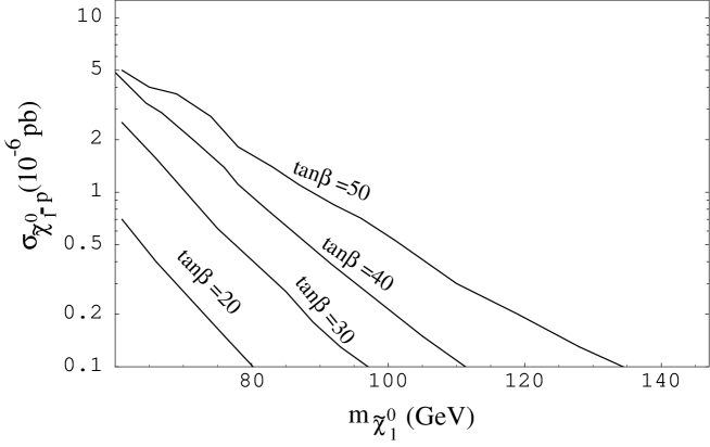
FIG. 3.: The maximum value of $\sigma_{\tilde{\chi}_{1}^{0}-p}$ vs. $m_{\tilde{\chi}_{1}^{0}}$ for $\tan{\beta}=20$, 30, 40, and 50 for Set 2 parameters of Eq. (12).

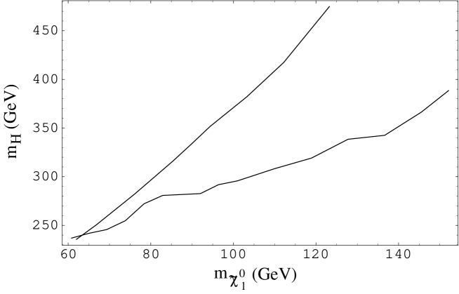
FIG. 4.: $m_{H}$ vs. $m_{\tilde{\chi}_{1}^{0}}$ when $\sigma_{\tilde{\chi}_{1}^{0}-p}$ takes on its maximum value. Top curve is for $\tan{\beta}=30$, bottom curve for $\tan{\beta}=50$.

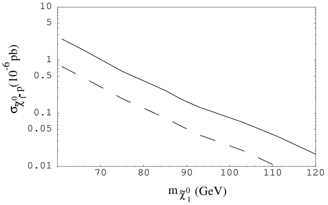
FIG. 5.: Maximum $\sigma_{\tilde{\chi}_{1}^{0}-p}$ vs. $m_{\tilde{\chi}_{1}^{0}}$ for $\tan{\beta}=30$ for Set 2 parameters (solid), and Set 1 parameters (dashed). See Eq. (12).

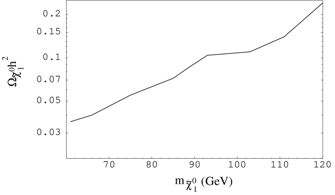
FIG. 6.: $\Omega_{\tilde{\chi}_{1}^{0}}h^{2}$ vs. $m_{\tilde{\chi}_{1}^{0}}$ for $\tan{\beta}=30$.

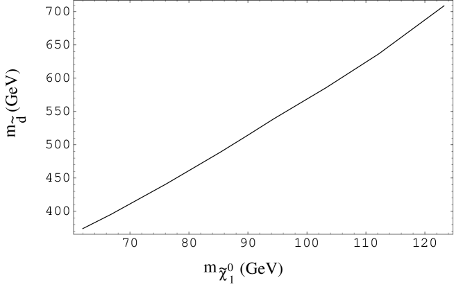
FIG. 7.: $m_{\tilde{d}}$ vs. $m_{\tilde{\chi}_{1}^{0}}$ for $\tan{\beta}=30$ when $\sigma_{\tilde{\chi}_{1}^{0}-p}$ takes on its maximum value.

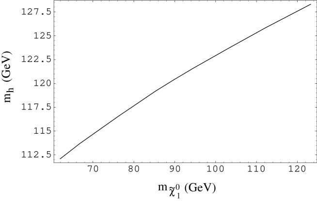
FIG. 8.: $m_{h}$ vs. $m_{\tilde{\chi}_{1}^{0}}$ for $\tan{\beta}=30$ when $\sigma_{\tilde{\chi}_{1}^{0}-p}$ takes on its maximum value.

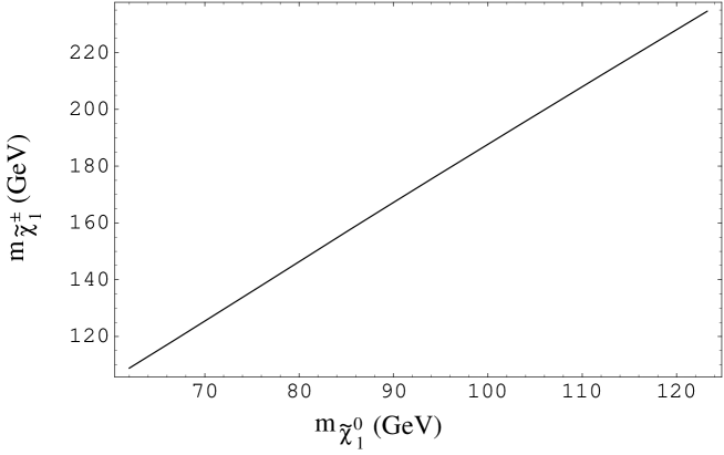
FIG. 9.: $m_{\tilde{\chi}_{1}^{\pm}}$ vs. $m_{\tilde{\chi}_{1}^{0}}$ for $\tan{\beta}=30$ when $\sigma_{\tilde{\chi}_{1}^{0}-p}$ takes on its maximum value.

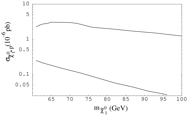
FIG. 10.: Maximum value of $\sigma_{\tilde{\chi}_{1}^{0}-p}$ vs. $m_{\tilde{\chi}_{1}^{0}}$ for $\tan{\beta}=7$ for nonuniversal soft breaking (upper curve) and universal soft breaking (lower curve).

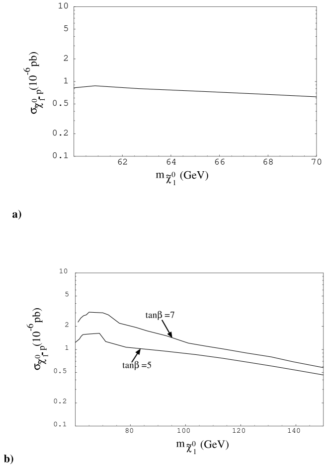
FIG. 11.: Maximum value of $\sigma_{\tilde{\chi}_{1}^{0}-p}$ vs. $m_{\tilde{\chi}_{1}^{0}}$ for a. $\tan{\beta}=3$, and b. $\tan{\beta}=5$, 7 for nonuniversal soft breaking. Note that the $\tan{\beta}=3$ curve terminates at $m_{\tilde{\chi}_{1}^{0}}\stackrel{{\scriptstyle\sim}}{{=}}$ 70 GeV.

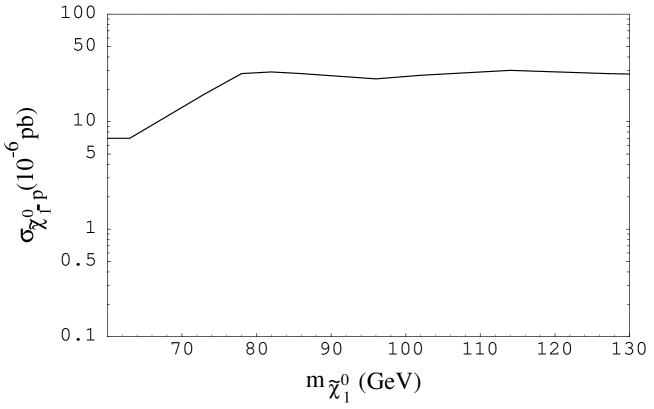
FIG. 12.: Maximum value of $\sigma_{\tilde{\chi}_{1}^{0}-p}$ vs. $m_{\tilde{\chi}_{1}^{0}}$ for $\tan{\beta}=15$ for nonuniversal soft breaking.

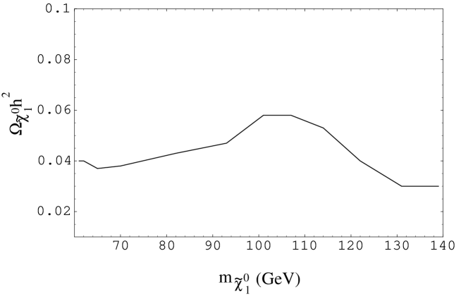
FIG. 13.: $\Omega_{\tilde{\chi}_{1}^{0}}h^{2}$ vs. $m_{\tilde{\chi}_{1}^{0}}$ for maximum $\sigma_{\tilde{\chi}_{1}^{0}-p}$ for $\tan{\beta}=7$, nonuniversal soft breaking.

FIG. 14.: $m_{H}$ vs. $m_{\tilde{\chi}_{1}^{0}}$ for maximum $\sigma_{\tilde{\chi}_{1}^{0}-p}$ for $\tan{\beta}=7$, nonuniversal soft breaking.

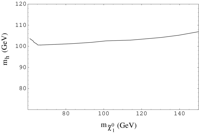
FIG. 15.: $m_{h}$ vs. $m_{\tilde{\chi}_{1}^{0}}$ for maximum $\sigma_{\tilde{\chi}_{1}^{0}-p}$ for $\tan{\beta}=7$, nonuniversal soft breaking.

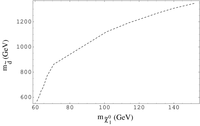
FIG. 16.: $m_{\tilde{d}}$ vs. $m_{\tilde{\chi}_{1}^{0}}$ for maximum $\sigma_{\tilde{\chi}_{1}^{0}-p}$ for $\tan{\beta}=7$, nonuniversal soft breaking.

FIG. 17.: Example of $p$-decay diagram. The major contribution comes from the second generation loop (i=2), the third generation contributing $\approx 30\%$ correction with arbitrary relative phase.

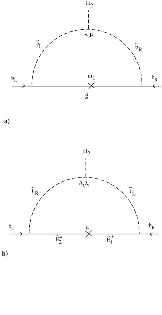
FIG. 18.: One loop correction to $b$-mass.

REFERENCES

• [1] A.H. Chamseddine, R. Arnowitt and P. Nath, Phys. Rev. Lett. 49, 970 (1982). For reviews see P. Nath, R. Arnowitt and A.H. Chamseddine, “Applied N=1 Supergravity” (World Scientific, Singapore, 1984); H.P. Nilles, Phys. Rep. 110, 1 (1984); R. Arnowitt and P. Nath, Proc. of VII J.A. Swieca Summer School (World Scientific, Singapore, 1994).
• [2] R. Arnowitt and P. Nath, Phys. Rev. D54, 2374 (1996).
• [3] T. Falk, K.A. Olive and M. Srednicki, Phys. Lett. B339, 248 (1994).
• [4] H. Goldberg, Phys. Rev. Lett. 50, 1419 (1983); J. Ellis, J.S. Hagelin, D.V. Nanopoulos, K. Olive and M. Srednicki, Nucl. Phys. B238, 453 (1984).
• [5] M. Goodman and E. Witten, Phys. Rev. D31, 3059 (1985).
• [6] M. Drees and N. Nojiri, Phys. Rev. D48, 3483 (1993).
• [7] A. Bottino, F. Donato, N. Fornengo and S. Scopel, Phys. Rev. D59, 095003 (1999).
• [8] M. Brhlik and L. Roszkowski, hep-ph/9903468.
• [9] P. Belli et.al., hep-ph/9903501.
• [10] A. Bottino, F. Donato, N. Fornengo and S. Scopel, hep-ph/9909228.
• [11] S. Kelley, J. Lopez, D. Nanopoulos, H. Pois and K. Yuan, Phys. Rev. D47, 246 (1993).
• [12] R. Arnowitt and P. Nath, Phys. Rev. Lett. 70, 3696 (1994).
• [13] G. Kane, C. Kolda, L. Roszkowski and J. Wells, Phys. Rev. D49, 6173 (1994).
• [14] H. Baer and M. Brhlik, Phys. Rev. D53, 597 (1996).
• [15] R. Arnowitt and P. Nath, Phys. Rev. D54, 2374 (1996).
• [16] H. Baer and M. Brhlik, Phys. Rev. D55, 3201 (1997).
• [17] H. Baer and M. Brhlik, Phys. Rev. D57, 567 (1998).
• [18] V. Barger and C. Kao, Phys. Rev. D57, 3131 (1998).
• [19] J. Ellis, T. Falk, K. Olive and M. Srednicki, hep-ph/9905481.
• [20] V. Berezinsky, A. Bottino, J. Ellis, N. Fornengo, G. Mignola and S. Scopel, Astropart. Phys. 5, 1 (1996).
• [21] V. Berezinsky, A. Bottino, J. Ellis, N. Fornengo, G. Mignola and S. Scopel, Astropart. Phys. 6, 333 (1996).
• [22] P. Nath and R. Arnowitt, Phys. Rev. D56, 2820 (1997).
• [23] R. Arnowitt and P. Nath, Phys. Lett. B437, 344 (1998).
• [24] A. Bottino, F. Donato, N. Fornengo and S. Scopel, Phys. Rev. D59, 095004 (1999).
• [25] R. Arnowitt and P. Nath, Phys. Rev. D60, 044002 (1999).
• [26] R. Bernabei et al., Phys. Lett. B424 (1998) 195; Phys. Lett. B450 (1999) 448.
• [27] See e.g. V. Barger, M.S. Berger and P. Ohmann, Phys. Rev. D49, 4908 (1994).
• [28] M. Brhlik, L. Everett, G. Kane, and J. Lykken, hep-ph/9908326.
• [29] E. Accomando, R. Arnowitt and B. Dutta, hep-ph/9909333.
• [30] H. Anlauf, Nucl. Phys. B430, 245 (1994).
• [31] Particle Data Group, European Physical Journal, C3, 1 (1998).
• [32] Super Kamiokande Collaboration, Phys. Rev. Lett. 83, 1529 (1999).
• [33] W. Freedman, astro-ph/9909076.
• [34] S. Dodelson and L. Knox, astro-ph/9909454.
• [35] J. Mohr, B. Mathiesen and A.E. Evrad, Astrophys. J. 517, 627 (1999).
• [36] S. Perlmutter et.al., Astrophys. J. (in press) (astro-ph/9812133); A.G. Riess et.al., Astron. J. 116, 1009 (1998).
• [37] C. Lineweaver, astro-ph/9909301.
• [38] H. Leutwyler, Phys. Lett. B374, 163 (1996).
• [39] J. Ellis and R. Flores, Phys. Lett. B263, 259 (1991); B300, 175 (1993).
• [40] For reviews see G. Jungman, M. Kamionkowski and K. Greist, Phys. Rep. 267, 195 (1995); E.W. Kolb and M.S. Turner, “The Early Universe” (Addison-Wesley, Reading, 1990).
• [41] K. Greist and D. Seckel, Phys. Rev. D43, 3191 (1991); P Gondolo and G. Gelmini, Nucl. Phys. B360, 145 (1991).
• [42] R. Arnowitt and P. Nath, Phys. Lett. B299, 58 (1993); Erratum ibid B303, 403 (1993); P. Nath and R. Arnowitt, Phys. Rev. Lett. 70, 3696 (1993).
• [43] L. Roszkowski, Phys. Lett. B262, 59 (1991).
• [44] R. Arnowitt and P. Nath, Phys. Rev. Lett. 69, 725 (1992).
• [45] T. Goto and T. Nihei, Phys. Rev. D59, 115009 (1999).
• [46] R. Rattazi and U. Sarid, Phys. Rev. D53, 1553, (1996); M. Carena, M. Olechowski, S. Pokorski and C. Wagner, Nucl. Phys. B426, 269, (1994).
Refer to caption