hep-ph/0001015 FTUV/00-03 IFIC/00-03
Status of the MSW Solutions to the Solar Neutrino Problem

In this talk we present the results of an updated global analysis of two-flavor MSW solutions [1] to the solar neutrino problem in terms of conversions of $\nu_{e}$ into active or sterile neutrinos including the the full data set corresponding to the 825-day Super–Kamiokande data sample as well as to Chlorine, GALLEX and SAGE experiments.

It is already three decades since the first detection of solar neutrinos. It was realized from the very beginning that the observed rate at the Homestake experiment was far lower than the theoretical expectation based on the standard solar model with the implicit assumption that neutrinos created in the solar interior reach the earth unchanged, i.e. they are massless and have only standard properties and interactions. From the experimental point of view much progress has been done in recent years. We now have available the results of five experiments, the original Chlorine experiment at Homestake [2], the radio chemical Gallium experiments on pp neutrinos, GALLEX and SAGE [3], and the water Cherenkov detectors Kamiokande and Super–Kamiokande [4] which we summarize in Table 1.

Table 1: Measured rates for the Chlorine, Gallium ( in SNU) and Super–Kamiokande (in $10^{6}$cm${}^{-}2$s^-1) experiments together with the predictions from the SSM [6].

Rates SSM	pp	pep	hep	Be	B	N	O	F	Total	$R^{exp}$
Gallium	70.45	2.87	0.015	34.45	12.38	3.65	6.04	0.072	$130\pm 7$	$72.3\pm 5.6$
Chlorine	0.0	0.233	0.009	1.15	5.89	0.099	.37	.0044	$7.8\pm 1.1$	$2.56\pm 0.23$
Super–Kam	0.0	0.0	0.00049	0.0	5.2	0.0	0.0	0.0	$5.2\pm 0.9$	$2.45\pm 0.23$

Super–Kamiokande has been able not only to confirm the original detection of solar neutrinos at lower rates than predicted by standard solar models, but also to demonstrate directly that the neutrinos come from the sun by showing that recoil electrons are scattered in the direction along the sun-earth axis. We now have good information on the time dependence of the event rates during the day and night, as well as a measurement of the recoil electron energy spectrum. After 825 days of operation, Super–Kamiokande has also presented preliminary results on the seasonal variation of the neutrino event rates an issue which will become important in discriminating the MSW scenario from the possibility of neutrino oscillations in vacuum [5].

In our study we use the following observables:

• the three measured rates shown in Table 1

• Super–Kamiokande results on the zenith angular dependence of the event rates during 1 day and 5 night periods.

• Recoil e spectrum including the 2 points from obtained with the super low energy threshold below 6.5 GeV and 18 points with 6.5¡E¡15 MeV.

• Seasonal variation of the event rates measured in 8 periods of 1.5 months each.

We obtain the allowed value of the parameters and the corresponding CL for the different scenarios by a $\chi^{2}$ analysis, details of which can be found in Ref. [1].

In our calculations of the expected values for these observables we use as SSM the fluxes from Ref. [6] but we also consider departures of the SSM by allowing arbitrary ${}^{8}B$ and $hep$ fluxes. For the Chlorine and Gallium experiments we use improved cross sections $\sigma_{\alpha,i}(E)$ $(\alpha=e,\,x)$ from Ref. [7]. For the Super–Kamiokande experiment we calculate the expected signal with the differential cross section $d\sigma_{\alpha}(E_{\nu},\,T^{\prime})/dT^{\prime}$, that we take from [8] taking into account the finite energy resolution of the experiment which implies that the measured kinetic energy $T$ of the scattered electron is distributed around the true kinetic energy $T^{\prime}$ according to a resolution function which we take from [9].

Using the predicted fluxes from the BP98 model the $\chi^{2}$ for the fit to the three experimental rates is $\chi^{2}_{SSM}=62.4/3$dof what implies that the probability of the observations to be an statistical fluctuation of the SSM is lower than $10^{-8}$!!. One may wonder about the possible dependence of the quality of description on the specific solar model used. In order to address this issue we try to fit the data by allowing a free normalization of the dominant neutrino fluxes $pp$ ${}^{7}Be$ and ${}^{8}B$ only imposing the constraint that the luminosity of the sun is supplied by nuclear reactions among the light elements what implies a linear relation among the three normalizations. The best fit point corresponds to an unphysical situation with negative ${}^{7}Be$ neutrino flux. After constraining the fluxes to be positive we obtain that the best fit point occurs at ${}^{7}Be/^{7}Be_{SSM}=0$, $pp/pp_{SSM}=1.08$ and ${}^{8}B/^{8}B_{SSM}=0.53$ with $\chi^{2}_{min}=21.4/1$dof which implies that there is no acceptable fit with a CL better than $5\times 10^{-4}$%.

Next we test the possibility of describing the data in terms of an energy independent neutrino conversion probability as expected, for instance in models explaining all evidences for neutrino oscillations (from solar, atmospheric and LSND data) in terms of three massive neutrinos. We find the values listed in Table 2

Table 2: Fit to the three measured rates for energy constant $\nu_{e}\rightarrow\nu_{X}$ conversion probability

$\nu_{x}$ active	$P_{ee}^{best}$	$\chi^{2}_{min}$/dof	CL (%)
Fix ${}^{8}B$	0.49	11.7/2	99.71
Free ${}^{8}B$	0.49	11.3/1	99.92
$\nu_{x}$ sterile
Fix ${}^{8}B$	0.52	20.5/2	99.996
Free ${}^{8}B$	0.52	20.5/1	99.99993

As seen in the table all scenarios with constant survival probability are ruled out with a CL larger than 99 %.

We now consider the description in terms of matter enhanced neutrino oscillations via the MSW mechanism [10]. We use in this case the neutrino survival probabilities in the presence of matter given in Ref. [11]. We show in Fig .1 the allowed regions for oscillations into active and sterile neutrinos for different combinations of the observables. In Table 3 we give the location of the best fit point for the different regions as well as the corresponding CL.

Table 3: Best fit points and the corresponding AL for the different MSW solutions to the solar neutrino deficit for different combinations of observables

. rates rates+zenith rates+spectrum rates+zenith+spectrum+season MSW dof 1 6 18 30 $\Delta m^{2}$ $5.6\times 10^{-6}$ $5.0\times 10^{-6}$ $5.6\times 10^{-6}$ $5.1\times 10^{-6}$ SMA $\sin^{2}(2\theta)$ 0.0063 0.0063 0.005 0.0055 $\chi^{2}_{min}$ (%CL) 0.37 (55) 5.9 (56) 23.4 (83) 37.4 (83) $\Delta m^{2}$ $1.4\times 10^{-5}$ $4.5\times 10^{-5}$ $1.4\times 10^{-5}$ $3.6\times 10^{-5}$ LMA $\sin^{2}(2\theta)$ 0.67 0.8 0.67 0.79 $\chi^{2}_{min}$ (%CL) 2.92 (91) 7.2 (70) 22.5 (79) 35.4 (77) $\Delta m^{2}$ $1.3\times 10^{-7}$ $1.0\times 10^{-7}$ $1.0\times 10^{-7}$ $1.0\times 10^{-7}$ LOW $\sin^{2}(2\theta)$ 0.94 0.94 0.94 0.94 $\chi^{2}_{min}$ (%CL) 7.4 (99) 12.7 (95) 26.7 (91.5) 40. (90) $\Delta m^{2}$ $5.\times 10^{-6}$ $5.0\times 10^{-6}$ $5.\times 10^{-6}$ $5.\times 10^{-6}$ SMA $\sin^{2}(2\theta)$ 0.005 0.005 0.003 0.003 sterile $\chi^{2}_{min}$ (%CL) 2.6 (90) 8.1 (77) 26.3 (89) 40. (90)

Several comments are in order. First we see that for active neutrinos there are three allowed regions, the small mixing angle region (SMA), the large mixing angle region (LMA) and the low mass region (LOW). For sterile neutrinos only the SMA solution is allowed. This arises from the fact that unlike active neutrinos which lead to events in the Super–Kamiokande detector by interacting via neutral current with the electrons, sterile neutrinos do not contribute to the Super–Kamiokande event rates. Therefore a larger survival probability for ${}^{8}B$ neutrinos is needed to accommodate the measured rate. As a consequence a larger contribution from ${}^{8}B$ neutrinos to the Chlorine and Gallium experiments is expected, so that the small measured rate in Chlorine can only be accommodated if no ${}^{7}Be$ neutrinos are present in the flux. This is only possible in the SMA solution region, since in the LMA and LOW regions the suppression of ${}^{7}Be$ neutrinos is not enough.

As for the quality of the different solutions for the oscillations into active neutrinos we find that the different observables favour different solutions. The total rates favours the SMA solution while the inclusion of the zenith angular dependence favours the LMA solution as although small, some effect is observed in the zenith angle dependence which points towards a larger event rate during the night than during the day, and that this difference is constant during the night as expected for the LMA solution. In the SMA solution, however, the enhancement is expected to occur mainly in the fifth night. The spectral information is such that the oscillation hypothesis does not improve considerably the fit to the energy spectrum as compared to the no-oscillation hypothesis as the data is basically consistent with a flat distribution what is also in better agreement with the LMA and LOW solutions while the SMA predicts a continuously raising spectrum. Moreover, the observation of a possible seasonal variation of the higher energy event rates in Super–Kamiokande could also be accommodated in terms of the LMA solution to the solar neutrino problem [5]. So once all the observables are combined we find that all solutions are allowed at the 90 % CL. LMA and SMA give similar descriptions, the LMA being slightly favoured.

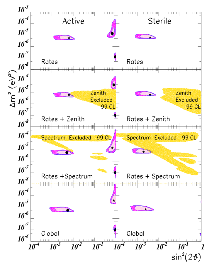
Figure 1: Allowed regions in $\Delta m^{2}$ and $\sin^{2}\theta$ from the combinations of the different observables as labeled in the figure for active-active (left column) and active-sterile transitions (right column). The darker (lighter) areas indicate 99% (90%)CL regions. Global (local) best–fit points are indicated by a star (dot). The shadowed areas in the second (third) row represent the region excluded by the zenith angle distribution (spectrum) data at 99% CL.

References

- [1] M. C. Gonzalez-Garcia, P. C. de Holanda, C. Peña-Garay, and J. W. F. Valle, hep-ph/9906469. To appear in Nuclear Physics B.
- [2] R. Davis, Jr, D. S. Harmer, and K. C. Hoffman, Phys. Rev. Lett. 20, 1205 (1968); B. T. Cleveland et al., Ap. J. 496, 505 (1998).
- [3] See talk by T. Kirsten in these proceedings.
- [4] See Talk by M. Nakahata in these proceedings.
- [5] P. C. de Holanda, C. Peña-Garay, M. C. Gonzalez-Garcia and J. W. F. Valle, Phys. Rev. D60 093010 (1999).
- [6] J.N. Bahcall, S. Basu and M. Pinsonneault, Phys. Lett. B433 (1998) 1.
- [7] http://www.sns.ias.edu/ jnb/SNdata
- [8] J. N. Bahcall, M. Kamionkowsky, and A. Sirlin, Phys. Rev. D51, 6146 (1995).
- [9] J. N. Bahcall, P. I. Krastev, and E. Lisi, Phys. Rev. C55, 494 (1997).
- [10] S.P. Mikheyev and A.Yu. Smirnov, Sov. Jour. Nucl. Phys. 42, 913 (1985); L. Wolfenstein, Phys. Rev. D17, 2369 (1978).
- [11] P.I. Krastev and S.T.Petcov, Phys. Lett. B207, 64 (1988); S.T.Petcov, Phys. Lett. B200, 373 (1988).