Abstract

A new gauge (m-gauge) condition is proposed by means of a generalization of the Maximal Abelian gauge (MAG). The new gauge admits a space time dependent embedding of the residual U(1) into the SU(2) gauge group. This embedding is characterized by a color vector $\vec{m}(x)$. It turns out that this vector only depends of gauge invariant parts of the link configurations. Our numerical results show color ferromagnetic correlations of the $\vec{m}(x)$ field in space-time. The correlation length scales towards the continuum limit. For comparison with the MAG, we introduce a class of gauges which smoothly interpolates between the MAG and the m-gauge. For a wide range of the gauge parameter, the vacuum decomposes into regions of aligned vectors $\vec{m}$. The ”neutral particle problem” of MAG is addressed in the context of the new gauge class.

 

^∗ supported by Graduiertenkolleg Struktur und Wechselwirkung von Hadronen und Kernen.

PACS: 11.15.Ha, 12.38.Aw

Dual Meissner effect, confinement, Abelian projection, gauge fixing, lattice gauge theory

1 Introduction

Revealing the mechanism which operates in Yang-Mills theories for confining quarks to color singlet particles is one of the most important tasks of modern quantum field theory. A knowledge of this mechanism will help to understand nuclear forces from first principles and will, e.g., have a strong impetus on the present understanding of hadron physics.

In the recent twenty years of active research, many proposals have been launched to explain quark confinement (see [1-7] for an incomplete list). Nowadays large scale computer simulations assign top priority to the so-called color superconductor mechanism [7]. This mechanism applies in the Abelian gauges [7], which allow for a residual U(1) gauge degree of freedom. Projection is performed to reduce the full SU(2) to compact U(1) gauge theory. After this projection, monopoles which carry quantized color-magnetic charges with respect to the residual U(1) group naturally appear as degrees of freedom [8]. The color-superconductor mechanism operates as follows: a condensation of these monopoles implies a (dual) Meissner effect. Color-electric flux is squeezed into flux tubes implying that the potential between two static color sources is linearly rising at large distances. Modern computer facilities provide the testing grounds: evidence has been accumulated that the dual superconductor picture captures parts of the roots of quark confinement [9, 10].

Unfortunately, the color-superconductor picture suffers from the following drawback: color states which are neutral with respect to the residual U(1) gauge are insensitive to the condensate of the color magnetic monopoles and therefore do not acquire a confining potential [11]. In this case, one would expect additional ”light” states in the particle spectrum besides hadrons and glueballs. This contradiction to the experiment requires a refinement of the dual superconductor picture. For this purpose, it was argued [11] that all color-magnetic monopoles which are defined by different Abelian projection schemes condense while only those monopoles which correspond to the gauge fixing at hand are manifest. The idea of the condensation of ”hidden” monopole degrees of freedom might conceptually solve the ”neutral particle problem”, but conceals the non-Abelian nature of the superconductor mechanism.

In this paper, we throw a new glance onto the non-Abelian Meissner effect by refraining from a residual U(1) gauge group which is uniquely embedded into the SU(2) gauge group all over space time. Instead of, space-time is decomposed into regions in each of which the embedding of the residual U(1) group into the SU(2) gauge group is chosen to yield the minimal error by a subsequent projection. Particles which are ”neutral” with respect to the U(1) subgroup in one particular region carry charge in another region. If the average over all configurations is performed during the Monte-Carlo sampling, all particles are confined on distances which exceed the intrinsic length scales of the regions.

For putting this idea on solid grounds, we propose a new type of gauge (referred to as m-gauge) which appears as a generalization of the Maximal Abelian gauge (MAG). In the m-gauge, the orientation of the U(1) subgroup in SU(2) is specified by a unit-color vector $\vec{m}$ which depends on space-time. In a first step, we show by means of numerical calculations that the m-projected theory still bears quark confinement at full strength. Secondly, for putting the m-gauge into a proper context, we investigate, by virtue of a gauge fixing parameter, a gauge fixing which smoothly interpolates between the MAG and the m-gauge. For a wide range of the gauge fixing parameters, the vacuum decomposes into regions of (approximately) aligned color vectors $\vec{m}$.

The paper is organized as follows: in the next section, we will introduce the novel type of gauge fixing and the corresponding projection. The numerical errors induced by projection are studied for the case of MAG and the case of m-gauge, respectively. In section 3, we reveal the color ferromagnetic correlations of the vector $\vec{m}$ present in the m-gauge. The interpolating gauges are introduced and the vacuum structure in these gauges is discussed. Conclusions are left to the final section.

2 M-gauge

2.1 The new gauge fixing and projection

A particular configuration of the SU(2) lattice gauge theory is represented by a set of link matrices $U_{\mu}(x)\,\in\,SU(2)$, which are transformed by a gauge transformation $\Omega(x)\,\in\,SU(2)$ into

$$U_{\mu}(x)\rightarrow U^{\Omega}_{\mu}(x)\;=\;\Omega(x)\,U_{\mu}(x)\,\Omega^{\dagger}(x+\mu)\;.$$ (1)

Our new proposal for the gauge fixing condition is given by

$$S_{\mathrm{fix}} = \frac{1}{2}\sum_{\mu,\,\{x\}}\;\hbox{tr}\left\{U^{\Omega}_{\mu}(x)\,m(x)\,\left(U^{\Omega}\right)^{\dagger}_{\mu}(x)\,m(x)\right\}\;\rightarrow\;\hbox{maximum}\;,$$ (2)

$$m(x) = m^{a}(x)\,\tau^{a}\;,\;\;\;\vec{m}^{T}(x)\vec{m}(x)=1\;,$$

where $\tau^{a}$ are the SU(2) Pauli matrices. For a given configuration $U_{\mu}(x)$ we allow for a variation of the gauge matrices $\Omega(x)$ and of the auxiliary unit vector $m^{a}(x)$ for maximizing the functional $S_{\mathrm{fix}}$. Note that a reflection of the vector, i.e., $\vec{m}(x)\rightarrow-\vec{m}(x)$, does not change the gauge fixing functional. Identifying the points $\vec{m}$ and $-\vec{m}$ of the sphere $S_{2}$ defines a projective space $RP_{2}$ which carries the gauge fixing information. Furthermore, $S_{\mathrm{fix}}$ is invariant under a multiplication of the gauge matrix $\Omega$, under consideration, with a center element of the SU(2) gauge group, i.e., $\Omega\rightarrow(-1)\,\Omega$. This implies that the theory after gauge fixing possesses a residual $Z_{2}$ gauge invariance, at least. It turns out that a further invariance is unlikely to exist for generic link configurations $U_{\mu}(x)$ (see discussion in subsection 2.2).

The concept of projection is to reduce the number of degrees of freedom while preserving the confining properties of SU(2) gauge theory. It might be easier in the reduced theory to reveal the mechanism of confinement than resorting to the full SU(2) gauge theory. In the present case, we define the projected links $\hat{U}_{\mu}(x)$ by

$$\hat{U}_{\mu}(x)\;:=\;N\,\left[U^{\Omega}_{\mu}(x)\;+\;m(x)\,U^{\Omega}_{\mu}(x)\,m(x)\,\right]\;,$$ (3)

where the normalization $N$ is obtained by demanding $\hat{U}_{\mu}(x)\,\hat{U}^{\dagger}_{\mu}(x)\,=\,1$.

It is convenient for an illustration of the gauge fixing (2) and the projection (3) to decompose the link variable as

$$U^{\Omega}_{\mu}(x)\;:=\;a_{\mu}^{(0)}(x)\;+\;i\,\vec{a}_{\mu}(x)\,\vec{\tau}\;,\hbox to28.45274pt{\hfill}\left(a_{\mu}^{(0)}(x)\right)^{2}\,+\,\vec{a}_{\mu}^{\;2}(x)\;=\;1\;\,\;\;\forall\mu,x$$ (4)

In this case, the gauge fixing condition $S_{\mathrm{fix}}$ (2) becomes

$$S_{\mathrm{fix}}\;=\;\sum_{\mu,\,\{x\}}\;\left\{\left(a_{\mu}^{(0)}(x)\right)^{2}\,-\,\vec{a}_{\mu}^{\;2}(x)\,+\,2\,\left(\vec{m}\vec{a}_{\mu}\right)^{2}\right\}\;\rightarrow\;\hbox{maximum}\;.$$ (5)

Representing the vector $\vec{a}_{\mu}(x)$ by components parallel to $\vec{m}(x)$ and perpendicular to $\vec{m}(x)$, i.e., $\vec{a}_{\mu}(x)=(a_{\mu}^{\parallel},a_{\mu}^{1\perp},a_{\mu}^{2\perp})^{T}$, the condition (5) is equivalent to

$$S_{\mathrm{fix}}\;=\;\sum_{\mu,\,\{x\}}\;\left\{1\;-\;2\left[\left(a_{\mu}^{1\perp}(x)\right)^{2}\,+\,\left(a_{\mu}^{2\perp}(x)\right)^{2}\right]\right\}\;\rightarrow\;\hbox{maximum}\;.$$ (6)

This equation tells us that the gauge fixing (2) minimizes the link components $\vec{a}_{\mu}(x)$ perpendicular to the vector $\vec{m}(x)$.

Inserting (4) in (3), one finds for the projected link variables

$$\hat{U}_{\mu}(x) = \;2N\,\left[a_{\mu}^{(0)}(x)\;+\;i\,\vec{m}(x)\vec{a}_{\mu}(x)\;\vec{m}(x)\vec{\tau}\,\right]$$ (7)

$$= 2N\,\left[a_{\mu}^{(0)}(x)\;+\;i\,a_{\mu}^{\parallel}(x)\;\vec{m}(x)\,\vec{\tau}\,\right]\;.$$ (8)

Projecting link configurations is a two-step process: firstly, one exploits the gauge degrees of freedom to minimize the link components $a_{\mu}^{1\perp}(x)$, $a_{\mu}^{2\perp}(x)$, perpendicular to $\vec{m}(x)$, and, secondly, these components $a_{\mu}^{1\perp}(x)$, $a_{\mu}^{2\perp}(x)$ are dropped for obtaining the projected link variable $\hat{U}_{\mu}(x)$. For quantifying the error of this projection, we introduce

$$\omega\;:=\;\frac{1}{N_{\mathrm{link}}}\,\left\langle S^{\mathrm{max}}_{\mathrm{fix}}[U]\right\rangle_{U}\;,$$ (9)

where $N_{\mathrm{link}}$ is the number of lattice links and $S_{\mathrm{fix}}^{\mathrm{max}}[U]$ is the maximum value of the gauge fixing functional $S_{\mathrm{fix}}$ (2) for a given link configuration $U_{\mu}(x)$. The brackets in (9) denote the Monte-Carlo average over all link configurations. An inspection of the equations (6) and (8) tells us that projection yields the exact result if $\omega$ possesses the largest value possible, i.e., $\omega=1$. The error increases if $\omega$ decreases.

Note that the space-time dependence of $m(x)$ relative to the link variables $U^{\Omega}_{\mu}(x)$ in the functional $S_{\mathrm{fix}}$ (2) is obtained by the demand for minimizing the error induced by projection. This demand dictates that $m(x)$ cannot be identified with a so-called Higgs field which figures in general Abelian gauges [12]. For an illustration of this fact, let $m(x)$, $\Omega(x)$ be the configurations which maximize $S_{\mathrm{fix}}[U]$ (2) for a given link configuration $U_{\mu}(x)$, and let assume that the fields $m(x)$, $\Omega(x)$ are uniquely defined (this is the generic case; see subsection 2.2). We introduce $U^{V}_{\mu}(x)$ as the link variables which are obtained from $U_{\mu}(x)$ by the gauge transformation $V(x)$, and repeat the gauge fixing procedure with the $U^{V}_{\mu}(x)$ as basis. If $m^{V}(x)$, $\Omega^{V}(x)$ denote the configurations which correspond to the maximum of $S_{\mathrm{fix}}[U^{V}]$, one finds $\Omega^{V}(x)=\Omega(x)\,V(x)$ and $m^{V}(x)=m(x)$. The later relation tells us that $m(x)$ only depends on the gauge invariant parts of the link variables $U_{\mu}(x)$, and therefore encodes physical information. By contrast, an auxiliary Higgs fields transforms homogeneously under the gauge transformation $V(x)$.

Let us compare our new gauge, defined by (2), with the Maximal Abelian gauge (MAG). The latter gauge can be obtained from the gauge condition (2) if one does not allow a variation of $m(x)$ with space time. For constant vectors $\vec{m}$, one might choose $\vec{m}$ to point in three direction in color space without a loss of generality. For an SU(2) gauge theory in four dimensions, one associates four link variables with each space time point, and therefore counts $12$ degrees of freedom at each lattice site ($9$ physical and $3$ gauge degrees of freedom). The MAG projection effectively reduces the SU(2) gauge theory to an U(1) one. After projection, the number of degrees of freedom per site is therefore $4$. In the new gauge, presented here, naive counting yields four Abelian links and the unit vector $\vec{m}(x)$, i.e., $6$ degrees of freedom at each site.

We finally comment on the Gribov problem to round out this subsection. Note that the following remarks also apply to the class of general Abelian gauges, and that, in particular, the practical problem in implementing the gauge is not a specialty of the new gauge proposed in the present letter. Although the gauge fixing starting from the condition (2) is conceptually free of Gribov ambiguities if one seeks out the global maximum of the functional $S_{\mathrm{fix}}$ (2), one recovers the Gribov problem in practice when the algorithm fails to detect the global maximum. In the context of variational gauges, several strategies have been proposed for evading this problem. One possibility is introducing a Laplacian version of the gauge fixing condition for adapting the problem to the numerical capabilities. Results are available in the literature for the case of Landau gauge [13], for the case of MAG [14] and for the case of the center gauge [15]. Another possibility is to introduce quantum gauge fixing [16] for putting the gauge fixing which is implemented by the algorithm in the proper context. Here, we will not perform a detailed study of the ”practical” Gribov problem in the context of the new gauge (2). In the present first investigation, we will only check whether the numerical results (see next section) are stable against random gauge transformations on the link variables before invoking the gauge fixing algorithm.

2.2 Quality of projection

Our numerical simulations were performed using the Wilson action and a lattice with $12^{4}$ space-time points. For $\beta$-values in the scaling window, i.e., $\beta\in[2.1,2.5]$, 200 heat–bath steps [17] were performed for initialization. When gauge fixing is requested by the application of interest, we used a standard iterative procedure with over-relaxation for finding the maximum value of the gauge fixing functional $S_{\mathrm{fix}}$ (2). Once we have obtained configurations $m(x)$, $\Omega(x)$ which maximize the functional $S_{\mathrm{fix}}$, we distort these configurations and re-handle the gauge fixing. Repeating this procedure (for a given link configuration $U_{\mu}(x)$) several times, we find unique fields $m(x)$, $\Omega(x)$ at the maximum of $S_{\mathrm{fix}}$. This provides numerical evidence that the (local) maximum of $S_{\mathrm{fix}}$ is stable against small gauge transformations, and that flat directions in the configuration space of $m(x)$, $\Omega(x)$ do not exist for generic link configurations. A thorough study of the Faddeev-Popov determinant in the case of m-gauge is requested for a rigorous proof of this fact. This is left to future work.

In a first investigation, we calculated the Creutz ratios $\chi_{kk}$ with help of the expectation values of quadratic Wilson loops of length $r=ka$, where $a(\beta)$ is the lattice spacing and $k$ is an integer. It is convenient for the extrapolation to the continuum limit to introduce the scale $\Lambda$ via

$$\Lambda^{2}\;=\;0.12\;\frac{1}{a^{2}(\beta)}\;\exp\left\{-\frac{6\pi^{2}}{11}\,\left(\beta-2.3\right)\;\right\}\;,$$ (10)

which is a renormalization group invariant quantity when one-loop scaling applies in the asymptotic $\beta$-region. The normalization of $\Lambda^{2}$ is chosen for reproducing the full SU(2) string tension, i.e. $\Lambda^{2}\rightarrow\sigma$ for $\beta\gg 2.1$.

Figure 1: Creutz ratios: fit to data of the full theory (solid line), m-projection (circles) and MAG projection (crosses).

Figure 1 shows our numerical data for $\chi_{kk}$ in units of $\Lambda^{2}$ as function of $r\,\Lambda$. It turns out that the data of the simulation employing the full SU(2) Wilson action is best fitted by (solid line)

$$\chi_{kk}\Lambda^{2}\;=\;\gamma_{1}+\;\gamma_{2}/r^{2}\;.$$ (11)

This ansatz for $\chi_{kk}$ is expected by relating Creutz ratios to the derivative of the static quark potential. The second term of the latter equation refers to the Coulomb interaction while the first term is present due to a non-vanishing string tension. Figure 1 also shows the data points for $\chi_{kk}$ calculated from links $\hat{U}_{\mu}(x)$ which are obtained from m-projection (see (7)). These data are contrasted with the result for $\chi_{kk}$ calculated with MAG projected links. In any case, the asymptotic, i.e. $r\Lambda\gg 1$, value for the string tension is reproduced within the numerical accuracy. A striking feature of figure 1 is that the data from m-projected links agree with the full result for the sizes $r$ explored in figure 1.

For a quantitative study of the error induced by projection, we calculated $\omega$ (9) for the case of the m-projection and the MAG projection, respectively (see table 1).

Table 1: The quality of projection, i.e., $\omega$ (9), as function of $\beta$.

$\beta$	$2.1$	$2.2$	$2.3$	$2.4$	$2.5$
$\omega$ [m-proj.]	$0.932(6)$	$0.934(4)$	$0.936(3)$	$0.938(3)$	$0.940(0)$
$\omega$ [MAG proj.]	$0.67(0)$	$0.68(4)$	$0.70(2)$	$0.72(1)$	$0.73(8)$

One observes that $\omega$ is much bigger for m-projection rather than for the case of MAG projection. In particular, the components of the (gauge fixed) links $U^{\Omega}$ which are dropped by projection, i.e. $U^{\Omega}\rightarrow\hat{U}$, are roughly of $5\%$ in size while the generic error due to projection in the case of MAG is of order $30\%$. One therefore expects that not only the string tension but also other physical observables which are calculated with m-projected links are well described. On one hand this feature is highly desired for constructing effective theories which cover a wide span of low energy properties of Yang-Mills theory. On the other hand, the introduction of additional degrees of freedom (compared with the case of MAG) obscures those ones which are responsible for confinement.

3 Color alignment in m-gauge

3.1 M-vector correlations

Figure 2: Raw data of the probability distribution of the scalar product $\eta$ between two neighboring color vectors $\vec{m}$ (left) and function $f(\eta)$ (right).

Let us assume that we are investigating a physical observable which possesses a correlation length $\xi$ by comparing the full with the m-projected theory. If the color vector $\vec{m}(x)$ is uniquely oriented in a space-time domain of size $l\gg\xi$, one would recover the standard MAG scenario (provided that $l$ is bigger than the scale set by the critical temperature, i.e., $l>0.7\,$fm, for detaining the Casimir effect). In particular, the dual superconductor picture would be expected operating if the string tension is the quantity of interest. For investigating the existence of such domains, and, in case, for relating the infra-red physics in the m-gauge to the well studied physics in MAG, a thorough study of the space-time correlations of the vectors $\vec{m}(x)$ is highly desired.

The space-time dependence of the gauge transformation $\Omega$ which maximizes the functional $S_{\mathrm{fix}}$ (2) induces a correlation of the unit vectors $\vec{m}(x)$ in space-time. For revealing these correlations, we numerically calculated the probability distribution of finding a particular scalar product $\eta$ of two vectors $\vec{m}$ located at neighboring sites of distance $a(\beta)$. The raw data of this distribution are shown in the left panel of figure 2. A random distribution of vectors would correspond to $dP/d\eta=1$. We clearly observe a maximum of the probability distribution at $\eta=1$. We find a color ferromagnetic correlation between the color vectors $\vec{m}(x)$. The value at the maximum position increases for increasing $\beta$, i.e., for a decreasing distance $a(\beta)$ between the neighboring vectors. This indicates that $\vec{m}(x)$ which constitutes a lattice vector model so far will become a smooth field in the continuum limit.

Figure 3: The scaling of the color ferromagnetic correlation length $L$.

For an interpretation of these results in the scaling limit $a(\beta)\rightarrow 0$, it is useful to parameterize the probability distribution as follows:

$$\frac{dP}{d\eta}\;=\;1\;+\;c\,\exp\left\{-\frac{a(\beta)}{L}\right\}\;f(\eta)\;,$$ (12)

where the function $f(\eta)$ satisfies without a loss of generality the constraints

$$\int_{0}^{1}f(\eta)\;d\eta\;=\;0\;,\hbox to28.45274pt{\hfill}f(1)=1\;.$$ (13)

The crucial finding is that the constants $L$ and $c$ as well as the function $f(\eta)$ are universal, i.e., independent of the renormalization point specified by $\beta$ (see figure 2 right panel and figure 3). Comparing the numerical data for $a(\beta)/L$ with the asymptotic one-loop $\beta$-dependence (dashed line in figure 3)

$$a(\beta)\;\approx\;0.16\,\hbox{fm}\,\exp\left\{-\frac{3\pi^{2}}{11}\beta\right\}$$ (14)

(where a string tension $\sigma=(440\>\mathrm{MeV})^{2}$ was used as reference scale), the extrapolation to the continuum limit yields

$$L\;=\;0.1(2)\,\hbox{fm}\;,\hbox to28.45274pt{\hfill}c\;=\;0.50(6)\;.$$ (15)

Note that for observing color ferromagnetic domains a probability distribution $dP/d\eta(\beta\rightarrow\infty)$ is required which diverges at $\eta=1$. However, our numerical data obtained in the scaling window $\beta\in[2.1,2.5]$ agree with a finite value for $dP/d\eta$ at $\eta=1$. Further numerical investigations (e.g. of the volume dependence of the distribution) are necessary for a definite conclusion on this issue.

In conclusion of this section, we find color ferromagnetic interactions between neighboring color vectors $\vec{m}$ which increase for decreasing distance $a(\beta)$ thus indicating that the vector field $\vec{m}(x)$ is smooth in the continuum limit. In the scaling limit, we find that these correlations extend over a range of roughly $0.12\,$fm. The color ferromagnetic interaction between the vectors is (most likely) not strong enough to induce the formation of color ferromagnetic domains in space-time.

3.2 Interpolating gauges

Figure 4: Quality of projection $\omega$ and the color ferromagnetic interaction strength $\mu$ (left panel); fraction of neighboring vectors with a scalar product larger than $0.95$ and $0.99$, respectively (right panel).

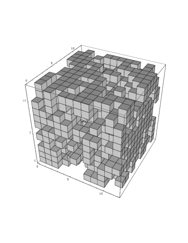
Figure 5: Spatial hypercube of one Monte-Carlo sample: region of aligned color vectors $\vec{m}(x)$ for $\kappa=0.6$.

Subsection 2.2 has demonstrated that the m-gauge is well adapted for projection. Unfortunately, the distribution of the auxiliary color vectors $\vec{m}(x)$ does not support an arrangement of these vectors in domains of constant orientation therefore impeding an interpretation of the m-gauge as local realization of MAG. For taking full advantage of the elaborated studies of physics in MAG [9, 10], we generalize the m-gauge condition (2) for allowing a smooth interpolation between the MAG and the m-gauge by virtue of a gauge fixing parameter $\kappa$. The generalized gauge fixing action  is

$$S_{\mathrm{fix}} = \frac{1}{2}\sum_{\mu,\,\{x\}}\;\hbox{tr}\left\{U^{\Omega}_{\mu}(x)\,m(x)\,\left(U^{\Omega}\right)^{\dagger}_{\mu}(x)\,m(x)\right\}$$ (16)

$$+ \kappa\,\sum_{\mu,\,\{x\}}\;\bigg{[}\vec{m}(x)\,\vec{m}(x+\mu)\biggr{]}^{2}\;\rightarrow\;\hbox{maximum}\;,$$ (17)

Note that the additional term (17) also respects the reflection symmetry $\vec{m}(x)\rightarrow-\vec{m}(x)$. For $\kappa=0$, one recovers the m-gauge (2). For $\kappa\gg 1$, on the other hand, there is a large penalty in action $S_{\mathrm{fix}}$ for non-uniformly oriented color vectors $\vec{m}$. One therefore obtains the MAG for sufficiently large $\kappa$. For quantifying the color ferromagnetic interaction strength, we introduce

$$\mu\;:=\;\frac{1}{N_{\mathrm{link}}}\,\sum_{\mu,\,\{x\}}\;\biggl{\langle}\,\vec{m}(x)\vec{m}(x+\mu)\,\biggr{\rangle}\;.$$ (18)

One finds $\mu=1/2$ for a random distribution of $\vec{m}\in RP_{2}$, and retrieves the MAG for $\mu=1$.

Figure 4 shows our numerical results for the ”quality of projection”, i.e. $\omega$ (9), and $\mu$ as function of $\kappa$ for a $12^{4}$ lattice and for $\beta=2.4$. As expected, the strength parameter $\mu$ gradually increases with rising $\kappa$ while $\omega$ monotonically decreases. The minimal error by projection is obtained in m-gauge ($\kappa=0$).

The strength parameter $\mu$ at large values of $\kappa$ indicate that regions of uniformly oriented color vector $\vec{m}$ form. Figure 4 also shows the fraction of vector pairs $\vec{m}(x)$, $\vec{m}(x+\mu)$ which possess a scalar product larger than $0.95$ ($0.99$). The data are obtained on $12^{4}$ lattice and for $\beta=2.4$. For illustrating the regions of aligned color vectors at large values of $\kappa$, figure 5 presents the spatial orientation of the color vectors $\vec{m}$ for one Monte-Carlo sample at a given time slice. The sample was obtained for $\kappa=0.6$. A reference vector was chosen at the center of the spatial hypercube. If the scalar product of a vector $\vec{m}$ located at the position $x$ with the reference vector exceeds $0.95$, an elementary cube which is spanned by the four points $x$, $x+\mu$, $\mu=1\ldots 3$ is marked. One observes that a particular region of (approximately) aligned vectors $\vec{m}$ is multi-connected and extends all over the lattice universe. This property of the regions of alignment does not match with its analog in solid state physics, i.e. the Weiss domains of ferromagnetism.

4 Conclusions

In the Maximal Abelian gauge (MAG), a uniquely oriented color vector $\vec{m}$ defines the embedding of the residual U(1) into the SU(2) gauge group. Evidence has been accumulated [9, 10] that in this case an (Abelian) dual Meissner effect confines particles which carry color-electric charge with respect to the U(1) subgroup. Since colored states which are, however, neutral from the viewpoint of the U(1) gauge group escape the confining forces provided by the dual superconductor mechanism, a refinement, i.e., a non-Abelian version, of the dual Meissner effect is highly desired. The concept of ”hidden monopoles” is one possibility [11].

By generalizing the MAG gauge condition, we have here proposed another possibility for a non-Abelian version of the dual Meissner effect. The new gauge (m-gauge) admits a space-time dependent embedding, characterized by the color vector $\vec{m}(x)$, of the residual U(1) into SU(2) gauge group. The space-time dependence of $\vec{m}(x)$ is self-consistently chosen to achieve the minimal error induced by projection. It turns out that the color vector $\vec{m}(x)$ does not change under ”small” gauge transformations of the link variable. Thus, the field $\vec{m}(x)$ carries gauge invariant information encoded in the link variables. Our numerical results show color ferromagnetic correlations of these vectors $\vec{m}$ which extends over a range of $\approx 0.1(2)\,$fm. The strength of these correlations seems to be too small for causing the formation of color ferromagnetic domains.

For relating the m-gauge to the MAG, we have introduced a class of gauges which smoothly interpolates between the MAG and the m-gauge by virtue of a gauge fixing parameter $\kappa$. For a wide span of $\kappa$, the vacuum decomposes into multi-connected regions which are characterized by uniquely oriented vectors, and which extend all over the lattice universe. The internal structure of these regions define an intrinsic lenght scale $l_{0}$. Each region bears the potential of an Abelian Meissner effect which operates with respect to the residual U(1) subgroup of SU(2). Colored states which do not feel a confining force in one particular region generically carry charge in another sector of space time. We speculate that, on performing the Monte-Carlo sampling, all colored states are confined on length scales bigger than the intrinsic size $l_{0}$ of the regions of color alignment. Note that the size $l_{0}$ is controlled by the gauge parameter $\kappa$. The request that the average size is a physical quantity defines the ”running” of the gauge parameter, i.e., the function $\kappa(\beta)$. The actual size of the regions of color alignment in physical units then defines the renormalized value $\kappa_{R}$ and must be provided by a renormalization condition.

In subsumption, for a class of gauge conditions, specified by a gauge parameter $\kappa>0$, the vacuum consists of regions of aligned color vectors $\vec{m}(x)$. The m-gauge appears as the limiting case $\kappa=0$. In this case, the error induced by projection is minimal at the expense of additional degrees of freedom as compared with the MAG. This fact renders the identification of the degrees of freedom relevant for quark confinement more difficult than in the MAG, but makes the m-gauge a convenient starting point for formulating an effective theory covering a wide span of low energy properties of SU(2) Yang-Mills theory.

Acknowledgments: We greatly acknowledge helpful discussions with M. Engelhardt, M. Quandt, H. Reinhardt and T. Tok. We are indebted to H. Reinhardt for support.

References

- [1] M. Baker, J. S. Ball and F. Zachariasen, Phys. Rev. D 51 (1995) 1968.
- [2] H. B. Nielsen and P. Olesen, Nucl. Phys. B160 (1979) 380; J. Ambjørn and P. Olesen, Nucl. Phys. B170 [FS1] (1980) 60; J. Ambjørn and P. Olesen, Nucl. Phys. B170 [FS1] (1980) 265; P. Olesen, Nucl. Phys. B200 [FS4] (1982) 381.
-
[3]
S. L. Adler, Phys. Rev. D 23 (1981) 2905;
S. L. Adler and T. Piran, Phys. Lett. B113 (1982) 405,
Phys. Lett. B117 (1982) 91;
W. Dittrich and H. Gies, Phys. Rev. D54 (1996) 7619. - [4] H. G. Dosch, Phys. Lett. B190 (1987) 177; H. G. Dosch and Yu. A. Simonov, Phys. Lett. B205 (1988) 339.
- [5] G. Fai, R.J. Perry and L. Wilets, Phys. Lett. B208 (1988) 1.
- [6] J. Polonyi, The Confinement and localization of quarks, In *Dobogokoe 1991, Proceedings, Effective field theories of the standard model* 337-357.
- [7] G. ’t Hooft, High energy physics , Bologna 1976; S. Mandelstam, Phys. Rep. C23 (1976) 245; G. ’t Hooft, Nucl. Phys. B190 (1981) 455.
- [8] A. S. Kronfeld, G. Schierholz, U.-J. Wiese, Nucl. Phys. B293 (1987) 461.
- [9] A. Di Giacomo, B. Lucini, L. Montesi and G. Paffuti, Colour confinement and dual superconductivity of the vacuum, I and II, hep-lat/9906024, hep-lat/9906025.
- [10] K. Schilling, G.S. Bali and C. Schlichter, Nucl. Phys. Proc. Suppl. 73 (1999) 638.
-
[11]
A. Di Giacomo, Plenary talk given at 14th International
Conference on Ultrarelativistic Nucleus-Nucleus Collisions (QM 99),
Torino, Italy, May 1999, hep-lat/9907010;
A. Di Giacomo, B. Lucini, L. Montesi and G. Paffuti, hep-lat/9906024. - [12] see e.g., O. Jahn, hep-th/9909004.
-
[13]
J. C. Vink and U. Wiese, Phys. Lett. B289 (1992)
122.
J. C. Vink, Phys. Rev. D51 (1995) 1292. - [14] A. J. van der Sijs, Nucl. Phys. Proc. Suppl. 53 (1997) 535, Nucl. Phys. Proc. Suppl. 73 (1999) 548.
- [15] C. Alexandrou, M. D’Elia and P. de Forcrand, Presented at 17th International Symposium on Lattice Field Theory (LATTICE 99), Pisa, Italy, 29 Jun - 3 Jul 1999, hep-lat/9907028.
- [16] K. Langfeld, M. Engelhardt, H. Reinhardt and O. Tennert, Presented at 17th International Symposium on Lattice Field Theory (LATTICE 99), Pisa, Italy, 29 Jun - 3 Jul 1999, hep-lat/9908026.
- [17] M. Creutz, Phys. Rev. D21 (1980) 2308.