Analytic Calculation of the 1-loop effective action for the O($\mathcal{N}+1$)-symmetric 2-dimensional nonlinear $\sigma$-model

Abstract

Starting from the 2-dimensional nonlinear $\sigma$-model living on a lattice $\Lambda$ of lattice spacing $a$ with action $S[\phi]=-\frac{1}{2}\beta\int_{z}\,\phi\triangle\phi,\quad\phi(z)\in S^{\mathcal{N}}$ we compute the Wilson effective action $S_{\mathrm{eff}}[\Phi]$ on a lattice of lattice spacing $\tilde{a}$ in a 1-loop approximation for a choice of blockspin $\Phi(x)=C\phi(x)\equiv\mathcal{C}\phi(x)/{|\mathcal{C}\phi(x)|}$, where $\mathcal{C}$ is averaging of $\phi(z)$ over a block $x$. We use a $\delta$-function constraint to enforce $\Phi=C\phi$. We consider also a Gaussian in place of the $\delta$-function in order to improve locality properties of $S_{\mathrm{eff}}$ as proposed by Hasenfratz and Niedermayer.

The result for $S_{\mathrm{eff}}$ is composed of the classical perfect action with a renormalized coupling constant $\beta_{\mathrm{eff}}$, an augmented contribution from a Jacobian, and further correction terms. The jacobian term depends on $\Psi(z)\cdot\Phi(x)$ where $\Psi$ is the interpolation of $\Phi$ with minimal action. The further correction terms include $\Psi\cdot\Phi$-dependent fluctuations of $\beta_{\mathrm{eff}}$ and a genuine 1-loop correction which depends on the matrix $\Psi\nabla_{\mu}\Psi^{T}(z)$ at two different sites $z=z_{1},z_{2}$. We find an analytic approximation for $\Psi$. Using it one can express the classical perfect action and $S_{\mathrm{eff}}$ as a function of the block spin $\Phi$. Our result extends Polyakovs calculation which had furnished those contributions to the effective action which are of order $\ln\tilde{a}/a$.

1 Introduction. Perfect actions

Perfect actions are actions for a lattice field theory which reproduce the expectation values of a continuum theory or of a theory with a much higher UV cutoff for a restricted class of “low energy”observables. Effective lattice actions in the sense of Wilson are perfect actions in this sense. Different approximations to the Wilson effective action have been given names such as classical perfect actions, 1-loop perfect actions etc. [14, 15].

In this paper we compute the effective lattice action for the 2-dimensional $O(\mathcal{N}+1)$-symmetric nonlinear $\sigma$-model in a 1-loop approximation. The result is given in eqs.(10)ff below. A summary was presented in [17].

The model lives on a quadratic lattice $\Lambda$ of lattice spacing $a$ with points typically denoted $z,w,\dots.$ Let $\hat{\mu}$ be the lattice vector of length $a$ in $\mu$-direction ($\mu=1,2$). We use lattice notations as follows (and similarly for the block lattice below).

$$\int_{z}(\dots) = a^{2}\sum_{z\in\Lambda}(\dots);$$ (1)

$$\qquad\nabla_{\mu}f(z) = \frac{1}{a}[f(z+\hat{\mu})-f(z)]=-\nabla_{-\mu}f(z+\hat{\mu});$$ (2)

$$\qquad-\triangle = \sum_{\mu=1,2}\nabla_{\mu}\nabla_{-\mu}\ .$$ (3)

In the continuum limit $a\to 0$, $\int_{z}\to\int d^{2}z$. The field $\phi(z)\in S^{\mathcal{N}}$ is a ($\mathcal{N}+1$)-dimensional unit vector, and $d\phi$ is the normalized uniform measure on the sphere. The action of the model is

$$S[\phi]=\frac{\beta}{2}\int_{z}[\nabla_{\mu}\phi(z)]^{2}=-\frac{\beta}{2}\int_{z}\phi\triangle\phi.$$ (4)

A block lattice $\tilde{\Lambda}$ of lattice spacing $\tilde{a}=s\cdot a$ is superimposed ($s$ positive integer). Its points are typically denoted $x,y,\dots.$ They are identified with squares of sidelength $\tilde{a}$ in $\Lambda$. There are $s^{2}$ points $z\in x$.

We define a blockspin $\Phi(x)$ which lives on the block lattice as a function $\Phi(x)=C\phi(x)$ of the fundamental field. $\Phi(x)$ is also a ($\mathcal{N}$+1)-unit vector; therefore the operator $C$ is necessarily nonlinear. We choose

$$\Phi(x)=C\phi(x)\equiv\frac{\mathcal{C}\phi(x)}{|\mathcal{C}\phi(x)|}\ ,$$ (5)

where $\mathcal{C}$ is a linear operator which averages over blocks. We take

$$\mathcal{C}\phi(x)={\mathrm{av}}_{z\in x}\phi(z)\equiv\tilde{a}^{-2}\int_{z\in x}\phi(z).$$ (6)

The Wilson effective action is defined by

$$e^{-S_{\mathrm{eff}}[\Phi]} = \int\,\mathcal{D}\phi\prod_{x}\delta(C\phi(x),\Phi(x))e^{-S[\phi]}\ ;$$ (7)

$$\mathcal{D}\phi = \prod_{z}d\phi(z),$$ (8)

where $d\phi$ is the uniform measure on the sphere $S^{\mathcal{N}}$, and $\delta$ is the $\mathcal{N}$-dimensional $\delta$-function on the sphere, viz.

$$\int\,d\phi_{1}f(\phi_{1})\delta(\phi_{1},\phi_{2})=f(\phi_{2})$$

for test functions on the sphere.

We use a $\delta$-function constraint because computation of expectation values of observables which depend on $\phi$ only through the blockspin $\Phi$ must then be identical whether computed with $S$ or $S_{\mathrm{eff}}$. This prepares best for stringent tests of the accuracy of the result.

Hasenfratz and Niedermayer [14] showed numerically that much better locality properties of effective actions are obtained when a Gaussian is used in the definition of the effective action in place of a sharp $\delta$-function.

This motivates us to examine also a larger class of block spin transformations which depends on a parameter $\kappa$ and which use a Gaussian in place of a $\delta$-function. The $\delta$-function constraint is obtained in the limit $\kappa\mapsto\infty$.

The calculation proceeds in the same way as in the $\kappa=\infty$ case, and the result is also the same, except

• The interpolation kernels $\mathcal{A}$ and high frequency propagators $\Gamma$ with finite $\kappa$ must be used throughout.

• The background field $\Psi$ is determined by eq.(148) of section 7, but the analytic expression for $\Psi$ remains valid when the finite-$\kappa$ expressions for $\mathcal{A}$ and $\Gamma$ are used.

• the classical perfect action differs from $S(\Psi)$ by an extra term
  $\frac{1}{2}\beta\kappa\int_{x}|\mathcal{C}\Psi^{\perp}(x)|^{2},$ where $\Psi^{\perp}(z)=\Psi(z)-\Phi(x)\left(\Psi(z)\cdot\Phi(x)\right)$ for $z\in x$.

• the jacobian $J_{0}$ receives extra contributions of order $\kappa^{-1}$.

Details are presented in section 7.

The analytic formula for the background field $\Psi$ elucidates the better locality properties of the effective action for suitable finite $\kappa$. It comes from the better locality properties of the Kupiainen Gawedzki high frequency propagator $\Gamma_{KG}$.

Background field and classical perfect action

Given a blockspin configuration $\Phi$, let $\Psi=\Psi[\Phi]$ be that field on the fine lattice $\Lambda$ which extremizes $S(\phi)+\frac{\tilde{\kappa}}{2}\sum_{x}|\mathcal{C}\phi^{\perp}(x)|^{2}$ subject to the constraints $|\Psi(z)|^{2}=1$ and

$$C\Psi=\Phi$$

$\Psi$ is called the background field. The classical perfect action is

$$S_{cl}[\Phi]=S(\Psi[\Phi]).$$ (9)

Here we wish to compute the 1-loop corrections. It is convenient to regard the full effective action as a function of $\Psi$. This is possible because $\Phi$ is determined by $\Psi$ according to eq.(1).

For large enough blocks, the background field $\Psi$ is smooth. An analytical approximation for $\Psi$ as a function of $\Phi$ is derived in section 6.

Summary of results

Because of the smoothness of $\Psi$, it sufficies to consider terms up to second order in $\nabla\Psi$. The exact 1-loop perfect action to this order is as follows.

$$S_{\mathrm{eff}} = S_{cl}-\sum_{x}\ln J_{0}(\mathcal{C}\Psi(x))-\frac{1}{2}Tr\ln\Gamma_{Q}$$ (10)

$$+\frac{1}{2}\int\left(\nabla_{\mu}\Psi^{T}(z)\beta_{\mathrm{eff}}^{1}(z)\nabla_{\mu}\Psi(z)+\beta_{\mathrm{eff}}^{2}(z)\frac{\Phi([z])^{T}(-\triangle)\Psi(z)}{\cos\theta(z)}\right)$$

$$+S_{\mathrm{eff}}^{(2)}+\int_{z}\mathrm{tr}\,j_{\mu}(z)\nabla_{\mu}\Gamma_{Q}(z,w)|_{w=z+\hat{\mu}}\ ;$$

$$j_{\mu}(z) = \Psi(z)\nabla_{\mu}\Psi^{T}(z)-\nabla_{\mu}\Psi(z)\Psi^{T}(z+\hat{\mu})+\Psi\Psi^{T}\nabla_{\mu}\Psi\Psi^{T}(z+\hat{\mu})\ ,$$ (11)

where $[z]$ is the block containing $z$, the jacobian is

$$J_{0}(\mathcal{C}\Psi(x))=|\Phi\cdot\mathcal{C}\Psi(x)|^{\mathcal{N}}$$ (12)

and $S_{\mathrm{eff}}^{(2)}$ is a contribution from a renormalized 1-loop graph with 2 vertices as follows

$$S_{\mathrm{eff}}^{(2)} = -\frac{1}{2}\int_{z}\int_{w}\mathrm{tr}\,\left(\nabla_{\mu}\Gamma_{Q}(z,w)\stackrel{{\scriptstyle\leftarrow}}{{\nabla}}_{\nu}j_{\nu}^{T}(w)\Gamma_{Q}(w,z)j_{\mu}(z)\right.$$ (13)

$$\qquad\qquad+\nabla_{\mu}\Gamma_{Q}(z,w)j_{\nu}(w)\nabla_{\nu}\Gamma_{Q}(w,z)j_{\mu}(z)$$

$$\left.\qquad\qquad+\ \delta_{\mu\nu}\delta(z-w)j_{\mu}(z)\Gamma_{Q}(z+\hat{\mu},z+\hat{\mu})j_{\nu}(z)\right)\ .$$

The $\delta_{\mu\nu}\delta(z-w)$-term subtracts the part which diverges in the limit $a\mapsto 0$. The last term in the definition (11) of $j_{\mu}$ is a lattice artifact and can be dropped inside eq.(13) because its contribution is actually of higher order in $\nabla\Psi$.

$\Gamma_{Q}$ is an $(\mathcal{N}+1)\times(\mathcal{N}+1)$ matrix propagator,

$$\Gamma_{Q}=\lim_{\kappa\mapsto\infty}(-\triangle+\kappa\hat{Q}^{T}\mathcal{C}^{\dagger}\mathcal{C}\hat{Q})^{-1}$$ (14)

with

$$\hat{Q}(z)=1-\Psi(z)\Psi^{T}(z)+\Phi(x)(\Psi^{T}(z)[1+\cos\theta(z)]-\Phi^{T}(x))\ ,$$ (15)

and

$$\cos\theta(z)=\Psi(z)\cdot\Phi(x)\ ,\ (x\ni z).$$ (16)

The coupling constant renormalizations $\beta_{\mathrm{eff}}^{1}$ and $\beta_{\mathrm{eff}}^{2}$ both have a residual dependence on $\Psi$ through $\hat{Q}$, so they fluctuate somewhat with $\Psi$; to leading order the dependence is through $\cos\theta$. Note that $\beta_{\mathrm{eff}}^{1}$ is a $(\mathcal{N}+1)\times(\mathcal{N}+1)$ matrix, while $\beta_{\mathrm{eff}}^{2}$ is a scalar.

$$\beta_{\mathrm{eff}}^{1}(z) = \Gamma_{Q}(z,z)\ ,$$ (17)

$$\beta_{\mathrm{eff}}^{2}(z) = -\mathrm{tr}\,[1-\Psi\Psi^{T}(z)]\Gamma_{Q}(z,z)\ .$$ (18)

Finally, the last term in eq.(10) is a lattice artifact; cp. Appendix B. and below.

Because of the complicated $\Psi$-dependence of the propagators, the exact result of the 1-loop calculation is too complicated to be of much practical use. Simple approximations require additional assumptions to justify them.

Assuming a smooth enough block spin field $\Phi(x)$, the matrix $\hat{Q}$ is close to $1$ and we may expand in powers of $\hat{Q}-1$. It will be shown in section 5.2 how to compute the corrections.

To leading order, the terms of order $\hat{Q}$ -1 will be neglected except in the $Tr\ln\Gamma_{Q}$-term, using

$$\Gamma_{Q}=\Gamma_{KG}{\bf 1}+O(\hat{Q}-1),$$ (19)

where $\Gamma_{KG}$ is the Kupiainen Gawedzki high frequency propagator for scalar fields as defined below. Splitting

$$[\cos\theta(z)]^{-1}\Phi(x)=\Psi+[\cos\theta(z)]^{-1}\Phi^{\perp}(z),$$ (20)

$(z\in x)$ where $\Phi^{\perp}$ is the component of $\Phi$ perpendicular to $\Psi$, the
$[\cos\theta(z)]^{-1}\Phi(x)\triangle\Psi$-term splits into a $\Psi\triangle\Psi$-term and a remainder which is small as a consequence of the maximizing condition on $\Psi$. It contains no $\ln\tilde{a}/a$ piece and is of higher order in $\hat{Q}-1$. As a result

$$S_{\mathrm{eff}} = -\sum_{x}\ln J_{0}(\mathcal{C}\Psi(x))-\frac{1}{2}Tr\ln\Gamma_{Q}+\frac{1}{2}\int_{z}\beta_{\mathrm{eff}}(z)|\nabla_{\mu}\Psi(z)|^{2}$$ (21)

$$+\mbox{renormalized 1-loop diagram}+\mbox{lattice artifacts}\ .$$

The sum of the first two terms will be called the augmented jacobian, the jacobian proper is given by eq.(12). The renormalized 1-loop diagram is the same as $S_{\mathrm{eff}}^{(2)}$ above, except that $\Gamma_{KG}$ is substituted for $\Gamma_{Q}$; moreover the last term in the definition (11) of $j_{\mu}$ may be dropped in $S_{\mathrm{eff}}^{(2)}$ because it is of order $a$. The effective coupling constant is

$$\beta_{\mathrm{eff}}(z)=-({\mathcal{N}-1})\Gamma_{KG}(z,z).$$ (22)

$\Gamma_{KG}(z,z)$ is very nearly constant except near block boundaries. Therefore we expect that the deviation of $\beta_{\mathrm{eff}}(z)$ from its block average can be neglected. Finally

lattice artifacts $$= \int_{z}\mathrm{tr}\,j_{\mu}(z)\nabla_{\mu}\Gamma_{KG}(z,w)|_{w=z+\hat{\mu}}$$

$$= -\frac{3}{8}\int_{z}|\nabla_{\mu}\Psi|^{2}(z)+O(a).$$

as $a\mapsto 0$. The lattice artifacts would vanish if $\Psi^{T}\nabla_{\mu}\Psi$ were zero as is true in the continuum. On the lattice it is $O(a)$, but nevertheless there remains a contribution when $a\mapsto 0$ because of the singularity of $\nabla_{\mu}\Gamma_{KG}$ at coinciding points. It amounts to a finite subtraction from the bare coupling constant.

Only the $\beta_{\mathrm{eff}}$-Term contributes to order $\ln\tilde{a}/a$, and we recover Polyakovs result in this approximation. Suppose the blockspin is reasonably smooth, so that $\Psi(z)-\Phi(x)$ may be regarded as a small quantity, of order $\epsilon$, and $\nabla_{x}\Phi(x)$ is also small, $o(\epsilon^{0})$.

Then $\hat{Q}-1$ is of order $\epsilon$. We expand $Tr\ln\Gamma_{Q}$ to order $\epsilon^{2}$.

To order $\epsilon^{2}$ the augmented jacobian comes out as the sum of $-\sum_{x}\ln J_{0}$, given by eq.(12), and

$$-\frac{1}{2}Tr\ln\Gamma_{Q} = \int_{x}\int_{z}\mathcal{A}_{KG}(z,x)\mathcal{C}(x,z)[\cos^{2}\theta(z)+\cos\theta(z)-2]$$ (24)

$$+\int_{z,w}\int_{x,y}\Psi^{\perp}(z)\cdot\Psi^{\perp}(w)[\Gamma_{KG}(z,w)\mathcal{C}^{\dagger}(w,x)u^{-1}(x,y)\mathcal{C}(y,z)$$

$$\quad\quad+\mathcal{A}_{KG}(z,x)\mathcal{C}(x,w)\mathcal{A}_{KG}(w,y)\mathcal{C}(y,z)]\ .$$

with $\mathcal{C}^{\dagger}(w,x)=\mathcal{C}(x,w)=\tilde{a}^{-2}$ if $w\in x$ and 0 otherwise. The jacobian proper and the first term of the augmentation are similar but they have a different ${\mathcal{N}}$-dependence.

In these formulas, $\mathcal{A}_{KG}$ and $\Gamma_{KG}$ are the Kupiainen-Gawedzki interpolation operator and high frequency propagator for scalar fields. For later use we indicate their definition for finite $\kappa$; a limit $\kappa\mapsto\infty$ can be taken at the end of the calculation. Let $v_{Cb}=(-\triangle)^{-1}$. Then

$$\mathcal{A}_{KG} = v_{Cb}\mathcal{C}^{\dagger}u^{-1}\ ,$$

$$u = \mathcal{C}^{\dagger}v_{Cb}\mathcal{C}\ +\frac{1}{\kappa},$$

$$\Gamma_{KG} = (-\triangle+\kappa\mathcal{C}^{\dagger}\mathcal{C})^{-1}$$

$$= (1-\mathcal{A}_{KG}\mathcal{C})v_{Cb}=v_{Cb}(1-\mathcal{C}^{\dagger}\mathcal{A}_{KG}^{\dagger})\ .$$

Their general properties and their Fourier representation for the special choice (6) of the averaging operator $\mathcal{C}$ are well known [10, 13, 22]. In particular, the propagators have exponential falloff with decay length of order one block lattice spacing $\tilde{a}$, and

$$\mathcal{C}\Gamma_{KG} = \frac{1}{\kappa}\mathcal{A}_{KG}^{\dagger}\mapsto 0,$$ (26)

$$\Gamma_{KG}\mathcal{C}^{\dagger}\ = \frac{1}{\kappa}\mathcal{A}_{KG}\mapsto 0.$$ (27)

$$\mathcal{C}\mathcal{A}_{KG} = 1-\frac{1}{\kappa}u^{-1}\mapsto 1.$$ (28)

The limit values are for $\kappa\mapsto\infty$. The Fourier components of these quantities are recorded in Appendix D. The coordinate space expressions can be evaluated by fast Fourier transformation. Software to do the computation and visualize the results has been provided by Max Griessl and Jan Würthner and can be downloaded from [23], together with some screenshots. A sample is shown below.

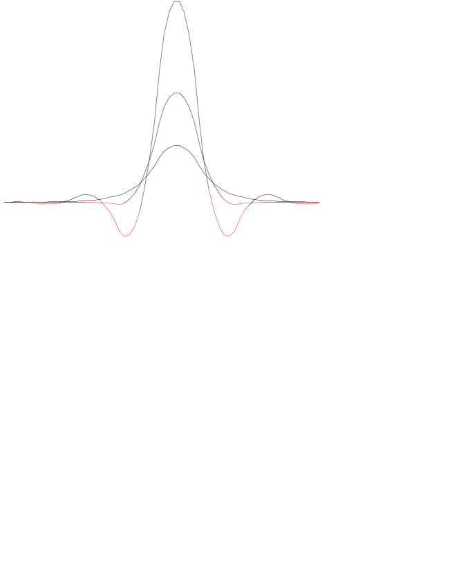
Figure 1: This figure shows cross sections through A-kernels with $\kappa$ values of 100 (top), $\frac{1}{8}$ (center) and $\frac{1}{32}$ (bottom). Note that the kernel oscillates for high $\kappa$ values.

In principle, a calculation of the 1-loop effective action for pure gauge theories along the same lines is feasible. The linearization of the block spin constraint and other ingredients were described in Balaban’s work [2] for general gauge group. The Fourier expansions of the interpolation kernel and high frequency propagators are also known, for a particular choice of block spin [18].

Note on the large field problem

Soon after rigorous work on the renormalization group started 20 years ago, it was recognized that one could not expect that the effective action would be local for completely arbitrary block spin configurations. This was termed the large field problem. A device to overcome this difficulty was proposed by Benfatto et al [4], and subsequently implemented in the work of Kupiainen and Gawedzki [11] and of Balaban [3]. It involves proofs that large fields in the above sense are very improbable. Fermi fields have no large field problem [8]

A large field problem can appear for fields which are not large in a naive sense. For instance, in 2-dimensional $\phi^{4}$-theory with a distinct mexican hat potential (pronounced maximum at $\phi=0$), the block spin $\Phi(x)\equiv 0$ is in the large field domain. Since $\Phi=0$ is translation invariant, the auxiliary theory, whose field is the fluctuation field, ought to respect symmetry under block lattice translations, with symmetry group $(\tilde{a}{\bf Z})^{2}$. Numerical work by Grießl [12] showed that the symetry was spontaneously broken (to $(2\tilde{a}{\bf Z})^{2}$). Such long range order in the auxiliary theory is incompatible with locality of the effective action.

The $\sigma$-model also has a large field problem for $\mathcal{N}>1$. Divide the block lattice in black and white squares in a checkerboard fashion and consider the configuration $\Phi(x)$ which points “up” (in +0 -direction) on white squares, and down on the black ones. A particular extremizing background field $\Psi$ has components

$$\Psi^{0}(z) = \cos(\pi(z^{1}+z^{2})/\tilde{a}),$$

$$\Psi^{1}(z) = \sin(\pi(z^{1}+z^{2})/\tilde{a}),$$

$$\Psi^{i}(z) = 0\qquad(i>1)\ .$$ (29)

But this is not unique. Continuous rotations in the space orthogonal to the 0-direction yield degenerate extrema. Therefore the auxiliary theory has a zero mode, its correlation functions will not decay quickly, and one cannot expect a local effective action for block spins very close to $\Phi$. But note that these are “energetically” the most unfavorable block spin configurations of all; they are near maxima of the effective action.

2 Linearization of the constraint

A perturbative calculation of the functional integral (7) for the effective action is not straightforward because the argument of the $\delta$-function is a nonlinear function of the field.

To solve this problem, we find a parametrization of an arbitrary field $\phi$ on $\Lambda$ in terms of the background field $\Psi=\Psi[\Phi]$ and a fluctuation field $\zeta$ such that the constraint becomes a linear constraint on $\zeta$.

$$\phi(z)=\phi[\Psi,\zeta](z)\ .$$ (30)

The background field is a smooth field. It represents the low frequency part of $\phi$, while $\zeta$ adds the high frequency contributions. $\zeta$ takes its values in a linear space. It has $\mathcal{N}$ components, and we choose it so that

$$\zeta(z)\perp\Phi(x)\ \mbox{for }z\in x\ .$$ (31)

Later, a further linear transformation to variables $\xi(z)\perp\Psi(z)$ is performed. There is a jacobian $J$ to the transformation, and the result has the form

$$e^{-S_{\mathrm{eff}}[\Phi]}=\int\prod_{z}d\zeta(z)\delta(\mathcal{C}\zeta)J(\Psi,\zeta)e^{-S(\phi[\Psi,\zeta])}.$$ (32)

Balaban [2] has shown how to find a suitable parametrization in the case of lattice gauge fields. His method is not applicable for the nonlinear $\sigma$-model for general $\mathcal{N}$, because it makes essential use of the fact that the field takes values in a group, and right and left multiplication of group elements commute, $(g_{L}g)g_{R}=g_{L}(gg_{R})$. But the suitable parametrization can be written down explicitly as follows.

Decompose $\phi(z)$ into components $\phi^{||}(z)$ and $\phi^{\perp}(z)$ parallel and perpendicular to $\Phi(x)$ for $z\in x$. The blockspin condition says that
$\mathcal{C}\phi(x)=\rho(x)^{-1}\Phi(x)$, where $\mathcal{C}$ is a linear block average, and the scalar factor $\rho(x)$ is determined by the requirement that $\Phi(x)$ has length 1. If we use the block average $\mathcal{C}$ defined in eq. (6) then only $\phi(z)$ with $z\in x$ enters into $\mathcal{C}\phi(x)$. The blockspin condition is therefore equivalent to

$$\mathcal{C}\phi^{\perp}(x)=0.$$ (33)

We parametrize

$$\phi^{\perp}(z) = \Psi^{\perp}(z)+\zeta(z),$$

$$\phi^{||}(z) = \left(1-\phi^{\perp}(z)^{2}\right)^{\frac{1}{2}}\Phi(x)$$ (34)

for $z\in x$. Since $\Psi$ satisfies the blockspin condition (33), the condition is equivalent to

$$\mathcal{C}\zeta(x)=0$$ (35)

The jacobian of the transformation will be worked out in Appendix A. The result is

$$J(\Psi,\zeta) = J^{0}(\mathcal{C}\phi)\prod_{z\in x}\left(1-(\Psi^{\perp}+\zeta)^{2}\right)^{-\frac{1}{2}},$$ (36)

$$J^{0}(\mathcal{C}\phi) = \prod_{x}J_{0}(\mathcal{C}\phi(x))=\prod_{x}(\Phi(x)\cdot\mathcal{C}\phi(x))^{\mathcal{N}}$$ (37)

As usual, $\Phi$ is regarded as determined by $\Psi$. In a 1-loop calculation, $J_{0}(\mathcal{C}\phi(x))$ is approximated by $J_{0}(\mathcal{C}\Psi(x))$. The last factor in $J$ will be cancelled when we transform to the $\xi$-variables.

3 The 1-loop approximation

The 1-loop approximation yields the effective action to order $\beta^{0}$. It is obtained by expanding the action to second order and the Jacobian to zeroth order in the fluctuation field. This approximates expression (32) by a Gaussian integral. The resulting $Tr\ log$ formula is not particularly useful, though.

It is possible to obtain a first simplification by exploiting the fact that the background field $\Psi$ is smooth. This is always true, whether the block spin $\Phi$ is smooth or not, provided the blocks are chosen large enough. A basic reason for this is that there are no domain walls in a 2-dimensional ferromagnet with continuous symmetry, because the free energy of such domain walls would decrease by making them wider. This is an old argument by M. Fisher [9] which was made mathematically precise by Dobrushin and Shlosman’s in their version of the proof of the absence of spontaneous breaking of continuous symmetries in 2 dimensions [7].

Because of the smoothness of $\Psi$ one can neglect terms of higher order than second in $\nabla\Psi$. Note however that this smoothness argument cannot be used to argue that $\cos\theta(z)=\Psi^{T}(z)\Phi(z)$ must alway be close to $1$. Only for sufficiently smooth block spin field $\Phi(x)$ will it be true that the component $\Psi^{\perp}(z)$ of $\Psi(z)$ which is perpendicular to $\Phi(x)$ is small.

The action $S$ involves derivatives of $\phi$ which contribute derivatives in $\zeta$. Because of the constraint $\zeta(z)\Phi(x)=0$ for $z\in x$, $\zeta$ will have jumps at block boundaries which contribute to the derivatives. In order to avoid this complication, it is convenient to make a further linear transformation from $\zeta(z)\perp\Phi(x)$ to variables $\xi(z)\perp\Psi(z)$,

$$\xi(z) = Q^{-1}(z)\zeta(z)\ ,$$ (38)

$$\xi(z)\Psi(z) = 0\ .$$ (39)

$Q(z)$ depends on $\Psi(z)$ and $\Phi(x)$. It is a linear transformation between different tangent spaces of the sphere

$$Q(z):T_{\Psi(z)}\mathcal{S}^{\mathcal{N}}\mapsto T_{\Phi(x)}\mathcal{S}^{\mathcal{N}}\ \mbox{for }z\in x.$$ (40)

The tangent spaces are $\mathcal{N}$-dimensional. We introduce the abbreviation

$$\pi(z)=1-\Psi(z)\Psi^{T}(z).$$ (41)

In covariant form, $Q$ is as follows

$$Q = \pi+\Phi(\Psi^{T}\cos\theta-\Phi^{T}),$$ (42)

$$Q^{-1} = 1-\frac{1}{\cos\theta}\Phi\Psi^{T}.$$ (43)

An expression in a particular basis will be given in appendix A.1. It shows that the modulus of the determinant of the resulting $\mathcal{N}\times\mathcal{N}$ matrix $Q(z)$ is

$$|\mbox{det}Q(z)|=\cos\theta(z)=(1-(\Psi^{\perp})^{2})^{\frac{1}{2}}.$$ (44)

Later on we shall introduce an extension of $Q$ to a map $\hat{Q}:\mathbf{R}^{\mathcal{N}+1}\mapsto\mathbf{R}^{\mathcal{N}+1}$.

The expansion of the field $\phi(z)$ in powers of $\xi$ comes out as

$$\phi(z)=\Psi(z)+\xi(z)-\frac{1}{2\cos\theta(z)}\xi(z)^{2}\Phi(x)+\dots$$ (45)

The action $S(\phi)$ can now be expanded up to second orders in $\xi$,

$$S(\phi)=S(\Psi)+\frac{1}{2}\xi S^{\prime\prime}(\Psi)\xi+\mbox{linear in $\xi$ }+\dots.$$ (46)

Now we are ready to consider the effective Boltzmann factor. In one loop approximation, i.e. to order $\beta^{0}$ the jacobian factor gets expanded to 0-th order in the fluctuation field. Furthermore

$$d\zeta(z)=|\mbox{det}Q(z)|d\xi(z)$$

and $\mbox{det}Q$ is as given above in eq.(44). Therefore the factor multiplying $J^{0}$ in the jacobian in (37) cancels out and we get to 1-loop order

$$e^{-S_{\mathrm{eff}}[\Phi]}=e^{-S(\Psi)}J^{0}(\mathcal{C}\Psi)\int\prod_{z}d\xi(z)\delta(\mathcal{C}Q\xi)e^{-\int_{z}\frac{\beta}{2}\left(\xi S^{\prime\prime}(\Psi)\xi\right)}$$ (47)

There is no linear term in $\xi$ in the exponent because $\Psi$ extremizes the action subject to the condition of fixed blockspin, and because $\xi$ parametrizes fields with the same blockspin.

The integration of the variable $\xi(z)$ is over the $\mathcal{N}$-dimentional tangent space $T_{\Psi(z)}\mathcal{S}^{\mathcal{N}}$, i.e. subject to the constraint

$$\Psi(z)\cdot\xi(z)=0.$$ (48)

The $\delta$-function $\delta(\mathcal{C}Q\xi)$ can be regarded as limit of a Gaussian. So we have to evaluate a Gaussian integral. As a result, one obtains the effective action as a sum of the classical action (tree perfect action) $S(\Psi)$, the jacobian term $-\ln J_{0}$ and a $Tr\ln\Gamma$-term. The propagator $\Gamma$ is the covariance of the above mentioned Gaussian measure.

This formula is not particularly illuminating because the full propagator $\Gamma$ has a complicated dependence on the field $\Psi$. It comes from three sources: The constraint (48) on $\xi$, the $\Psi$-dependence of $Q$, and finally the $\Psi$-dependence of $S^{\prime\prime}$.

A simplification is possible because the smoothness of the background field $\Psi$ (on lenght scale $a=$ lattice spacing of the fine lattice) can be exploited. In the approximation which exploits the smoothness of the background field $\Psi$ it is not necessary to consider terms of higher than second order in $\nabla_{\mu}\Psi$. $S^{\prime\prime}$ contains field dependent terms of first and second order in $\nabla\Psi$. They can be treated as perturbations which are treated by second and first order perturbation theory, respectively. This extracts the field dependence of $S^{\prime\prime}$ from the propagator.

The field dependence in $Q$ reflects the detailed choice of the block spin. Its contributions are not of order $\ln\tilde{a}/a$ and are therefore not included in Polyakovs result. The derivation of explicit formulas depends on the assumption that the block spin field $\Phi$ on the block lattice is smooth enough, or, more precisely, on sufficient smoothness of $\Psi$ on the lenght scale of the lattice spacing $\tilde{a}$ of the block lattice. There exists an extension of $Q$ to an $(\mathcal{N}+1)\times(\mathcal{N}+1)$ matrix $\hat{Q}$. When the assumption holds, $\hat{Q}$ is close to 1, and one can derive a power series expansion of the propagator in powers of $\hat{Q}-1$. We will later compute this expansion.

There remains the constraint $\Psi\cdot\xi=0$ on the integration variables $\xi(z)$. There are two ways to handle this

1. Polyakovs method. One expands $\xi(z)$ in a basis $e_{1}(z),\dots e_{\mathcal{N}}$ for the tangent space $T_{\Psi(z)}\mathcal{S}^{\mathcal{N}}$. In differential geometry, such a basis is called a moving frame. $S^{\prime\prime}$ becomes a $\mathcal{N}\times\mathcal{N}$ matrix in this basis.

   Polyakovs method has the advantage that the origin of the characteristic factor $\mathcal{N}-1$ in the formula for the running coupling constant emerges in a very transparent fashion from the form of $S^{\prime\prime}$. Therefore we show the details in the next section. The result agrees with Polyakovs’, to order $\ln\tilde{a}/a$.

   The disadvantage of Polyakov’s method is that the expansion of the propagator in powers of $\hat{Q}-1$ would be very thorny.

2. $\mathcal{N}+1$-dimensional integration. Here one inserts $1$ in the form of a Gaussian integral over an additional integration variable $\xi^{0}(z)\in{\bf R}$. This is combined with the $\mathcal{N}$-dimensional integration over $\xi(z)$ to an $\mathcal{N}+1$-dimensional integration over $\varphi(z)=\xi(z)+\xi^{0}\Psi(z)\in\mathbf{R}^{\mathcal{N}+1}$.

   In this formulation the power series expansion in $\hat{Q}-1$ is straightforward, but Polyakovs result must be extracted by evaluating the singular part of a 1-loop graph.

It is convenient to write the action in a gauge covariant form by introducing an arbitrary z-dependent basis. This yields results which can be used in both methods. The basis consists of an orthonormal set of vectors $e_{\alpha}(z)$, $\alpha=0,\dots\mathcal{N}$ for every site $z\in\Lambda$ which span $\mathbf{R}^{\mathcal{N}+1}$, so that

$$e_{\alpha}\cdot e_{\beta}(z)=\delta_{\alpha\beta}.$$ (49)

The field can be expanded in the basis

$$\phi(z)=\sum_{\alpha=0}^{\mathcal{N}}\phi^{\alpha}(z)e_{\alpha}(z).$$ (50)

and similarly for $\xi$ and $\Phi$. We assemble the expansion coefficients in $\mathcal{N}+1$ dimensional column vectors $\underline{\phi},\underline{\Psi},\underline{\Phi}$ and $\underline{\xi}$.

One introduces matrices $A_{\mu}(z)$ by

$$A_{\alpha\beta\mu}(z)=e_{\alpha}(z+\hat{\mu})\cdot\nabla_{\mu}e_{\beta}(z)$$ (51)

On the lattice, the Leibniz rule takes the form

$$\nabla_{\mu}(f(z)g(z))=(\nabla_{\mu}f(z))g(z)+f(z+\hat{\mu})\nabla_{\mu}g(z).$$ (52)

Using this one finds the following substitute for antisymmetry in indices $\alpha,\beta$,

$$A_{\alpha\beta\mu}(z)=A_{\beta\alpha-\mu}(z+\hat{\mu}).$$ (53)

The action takes the covariant form

$$|\nabla_{\mu}\phi|^{2}=|(\nabla_{\mu}+A_{\mu})\underline{\phi}|^{2}.$$ (54)

In a constant basis, one has $A_{\mu}=0$.

The expansion (45) carries over to the column vectors. Using it one computes with the help of the lattice Leibniz rule

$$|\nabla\underline{\phi}|^{2}(z)=|\nabla\underline{\Psi}|^{2}(z)+|\nabla\underline{\xi}|^{2}(z)+\frac{1}{\cos\theta(z)}\underline{\Phi}(x)\cdot\triangle\underline{\Psi}(z)\underline{\xi}^{2}(z)$$ (55)

with $\cos\theta(z)=\Psi(z)\cdot\Phi(x)$ as usual, $z\in x$. A total divergence has been omitted which arises from partial integration of a $\nabla\underline{\xi}^{2}$-term.

Because of the smoothness of $\Psi$, $\underline{\Phi}\cdot\triangle\underline{\Psi}$ is of order $|\nabla\Psi|^{2}$. To order $|\nabla\Psi|^{2}$ we find

$$\xi S^{\prime\prime}\xi=\int_{z}\left[|(\nabla_{\mu}+A_{\mu})\underline{\xi}|^{2}(z)+\frac{1}{\cos\theta(z)}\underline{\Phi}(x)\cdot\triangle\underline{\Psi}(z)\underline{\xi}^{2}(z)\right].$$ (56)

4 Polyakov’s method

In Polyakovs method one uses a basis with

$$e_{0}(z)=\Psi(z)\ .$$ (57)

The basis vectors $e_{1}(z),\dots e_{\mathcal{N}}(z)$ span the tangent space $T_{\Psi(z)}\mathcal{S}^{\mathcal{N}}$ and the $\xi$-field has no $0$-component.

There is a remaining arbitrariness in the choice of basis. The $O(\mathcal{N})$-group of those local rotations which leave $\Psi(z)$ invariant form a symmetry group of gauge transformations. The $\mathcal{N}\times\mathcal{N}$ matrices

$$a_{\mu}(z)=(A_{ij\mu}(z),\ i,j=1\dots\mathcal{N})$$ (58)

transform like gauge fields under these gauge transformations, while

$$A_{i0\mu}(z)=\left(\nabla_{\mu}\Psi(z)\right)^{i}$$ (59)

transform like $\mathcal{N}$-vector fields.

We compute the field strength tensor for the vector potential $a_{\mu}$,

$$F_{ij\mu\nu}(z) = \nabla_{\mu}a_{ij\nu}(z)-\nabla_{\nu}a_{ij\mu}(z)$$ (60)

$$+a_{ik\mu}(z+\nu)a_{kj\nu}(z)-a_{ik\nu}(z+\mu)a_{kj\mu}(z)\ .$$

Using the completeness relation for the basis in the form

$$\sum_{i=1}^{\mathcal{N}}e_{i}(z)e_{i}(z)^{T}=1-\Psi\Psi^{T}$$

one computes the component of the field strength tensor as

$$F_{ij\mu\nu}=e_{i}(z+\hat{\nu}+\hat{\mu})\nabla_{\mu}\Psi(z+\hat{\nu})e_{j}(z)\cdot\nabla_{\mu}\Psi(z)-(\mu\leftrightarrow\nu).$$ (61)

We see that the field strength tensor is of order $(\nabla\Psi)^{2}$. It follows that the vector potential $a_{\mu}$ in Lorentz gauge,

$$\nabla_{\mu}a_{\mu}=0\ ,$$

is also of order $(\nabla\Psi)^{2}$. The $[a_{\mu},a_{\nu}]$ term in expression (60) is negligible and the vector potential to leading order could be recovered as

$$a_{\nu}(z)=-\int_{w}\nabla_{\mu}v_{\mathrm{Cb}}(z-w)F_{\nu\mu}(w)\ .$$

Although the Coulomb potential $v_{\mathrm{Cb}}$ in 2 dimensions does not exist, its derivative is well defined.

Separating the terms which involve $a_{\mu}$ and $A_{0i\mu}$ and using the antisymmetry eq.(53) of $A$ and $\nabla_{-\mu}\Psi(z+\hat{\mu})=-\nabla_{\mu}\Psi(z)$ we obtain

$$|(\nabla_{\mu}+A_{\mu})\underline{\xi}|^{2}=|(\nabla_{\mu}+a_{\mu})\underline{\xi}|^{2}+|\xi\cdot\nabla_{\mu}\Psi|^{2}.$$ (62)

The last term involves the components $[\nabla\Psi]^{i}$ of $\nabla\Psi$ with respect to the moving frame, not $\nabla\Psi^{i}$.

In conclusion

$$\xi S^{\prime\prime}\xi=\int_{z}|(\nabla_{\mu}+a_{\mu})\underline{\xi}|^{2}(z)+\xi S_{I}^{\prime\prime}\xi$$ (63)

with

$$\xi S_{I}^{\prime\prime}\xi=\int_{z}\left([\xi\cdot\nabla_{\mu}\Psi]^{2}(z)+\xi^{2}(z)[\Psi\cdot\triangle\Psi](z)+\frac{1}{\cos\theta}\xi^{2}(z)[\Phi^{\perp}\cdot\triangle\Psi](z)\right).$$

The $\Phi\cdot\triangle\Psi$-term was split into two terms in order to single out the last term in $S_{I}^{\prime\prime}$. We will see later that this last term is very small for smooth enough block spin fields. This is a consequence of the extremizing property of $\Psi$. The term is $\triangle\Psi$ multiplied with an expression of order $(\Psi^{\perp})^{3}$, and turns out not to contribute at all to order $\ln\tilde{a}/a$.

The effective Boltzmann factor becomes

$$e^{-S_{\mathrm{eff}}[\Phi]}=e^{-S(\Psi)}\int\prod_{z}d\xi(z)\delta(\mathcal{C}Q\xi)J^{0}(\mathcal{C}\Psi)e^{-\int_{z}\frac{\beta}{2}\left([(\nabla_{\mu}+a_{\mu})\xi]^{2}+\xi S_{I}^{\prime\prime}(\Psi)\xi\right)}$$ (64)

The $\delta$-function can be regarded as limit of a Gaussian, and we have to evaluate a Gaussian integral.

Let us write $[z]\in\tilde{\Lambda}$ for the block $x$ which contains $z$. Let us remember that $Q(z)$ is a map (40) from $T_{\Psi(z)}\mathcal{S}^{\mathcal{N}}$ to $T_{\Phi(x)}\mathcal{S}^{\mathcal{N}}$, and $\mathcal{C}$ defines a map of functions on the fine lattice $\Lambda$ with values in $T_{\Phi([z])}\mathcal{S}^{\mathcal{N}}$ to functions on the block lattice with values in $T_{\Phi(x)}\mathcal{S}^{\mathcal{N}}$. Therefore the operator $Q^{T}\mathcal{C}^{\dagger}\mathcal{C}Q$ maps functions with values in $T_{\Psi(z)}\mathcal{S}^{\mathcal{N}}$ into functions of the same kind. The Polyakov basis elements $e_{i}(z),\ i=1\dots\mathcal{N}$ are a basis for $T_{\Psi(z)}\mathcal{S}^{\mathcal{N}}$. We denote by $P(z,w)=(P_{ij}(z,w),ij=1\dots\mathcal{N})$ the matrix of the kernel of $Q^{T}\mathcal{C}^{\dagger}\mathcal{C}Q$ with respect to this Polyakov basis, viz.

$$\int_{w}P_{ij}(z,w)\xi^{j}(w)=e_{i}(z)\cdot\left(Q^{T}\mathcal{C}^{\dagger}\mathcal{C}Q\xi\right)(z).$$ (65)

$P(z,w)$ is only nonzero when $z$ and $w$ belong to the same block $x$. The $\delta$-function becomes the limit of a Gaussian as follows

$$\delta(\mathcal{C}Q\xi) = \lim_{\kappa\mapsto\infty}N_{\kappa}e^{-\frac{\beta\kappa}{2}\int_{z}\int_{w}\xi^{i}(z)P_{ij}(z,w)\xi^{j}(w)}$$ (66)

$$N_{\kappa} = \left({\kappa a^{d}}/{2\pi}\right)^{\mathcal{N}/2}$$ (67)

Define the high frequency propagator (=propagator of the $\xi$-field) in the Polyakov basis

$$\Gamma^{e}_{\kappa}=\beta^{-1}\left(-[\nabla_{\mu}+a_{\mu}]^{2}+\kappa P\right)^{-1}$$ (68)

Now we can evaluate expression (64) for $S_{\mathrm{eff}}$ with volume element

$$d\xi(z)=d\xi^{1}(z)\dots d\xi^{\mathcal{N}}(z).$$

The result is

$$S_{\mathrm{eff}}[\Phi]=-\ln J^{0}(\mathcal{C}\Psi)+S(\Psi)+\frac{1}{2}\mathrm{tr}\,S_{I}^{\prime\prime}(\Psi)\Gamma^{e}_{\kappa}-\frac{1}{2}Tr\ln\Gamma^{e}_{\kappa}+const$$ (69)

in the limit $\kappa\mapsto\infty$. Note that $P$ depends on $\Psi$ because $Q$ depends on $\Psi$. Therefore the propagator $\Gamma^{e}_{\kappa}$ also has a residual $\Psi$ dependence. It is small when the block spin field is smooth, because the extension $\hat{Q}$ of $Q$ is in this case close to $1$. Unfortunately it would be difficult to find the first order term in $\hat{Q}-1$ in this formalism, because the formula for $P$ contains the moving frame, and because there could be a term which is first order both in $a_{\mu}$ and in $\hat{Q}-1$.

4.1 Recovery of Polyakov’s result

Polyakov determined the contributions to the effective action which are of order $\ln\tilde{a}/a$. They do not depend on the detailed form of the blockspin which fixes the infrared cutoff in the auxiliary theory with fields $\xi$. The term $\kappa P$ in the high frequency propagator has the effect of an infrared cutoff. This has been discussed in detail in the work of Kupiainen and Gawedzki [10]. To get the result modulo details of the choice of infrared cutoff, we may therefore replace $\kappa P$ by a mass term $M^{2}$, where $M=o(\tilde{a}^{-1})$.

The propagator also has a dependence on the $O(\mathcal{N})$-gauge field $a_{\mu}$. We show that this can be neglected, by exploiting the smoothness of the background field $\Psi$. We need only consider terms up to order $O([\nabla\Psi]^{2}).$ The result is gauge invariant. $a_{\mu}$ in Lorentz gauge is $O([\nabla\Psi]^{2})$ as we saw. A perturbation expansion in $a_{\mu}$ shows that $Tr\ln\Gamma^{e}=O(a_{\mu}^{2})$. Therefore the $a_{\mu}$ dependence of this term can be neglected. $S_{I}$ is already $O([\nabla\Psi]^{2})$, therefore the $a_{\mu}$-dependence in the propagator multiplying it can also be neglected. The high frequency propagator matrix can therefore be replaced by

$$\Gamma^{e}_{\kappa}(z,w)_{ij}\approx\beta^{-1}\delta_{ij}v_{M}(z-w)$$ (70)

where $v_{M}$ is the Yukawa potential in 2 dimensions with mass $M$ of order $\tilde{a}^{-1}$, viz.

$$v_{M}=(-\triangle+M^{2})^{-1}$$

The $Tr\ln$-term has become a constant. The jacobian is not ultraviolet divergent and is therefore a feature of the details of the infrared cutoff. Inserting $S_{I}^{\prime\prime}$ we get the result in the desired approximation

$$S_{\mathrm{eff}}[\Phi]=\frac{1}{2}\int_{z}(\beta-(\mathcal{N}-1)v_{M}(0))[\nabla_{\mu}\Psi(z)]^{2}+S_{\mathrm{isZero}},$$ (71)

with

$$S_{\mathrm{isZero}}=\frac{1}{2}\mathcal{N}v_{M}(0)\int_{z}[\cos\theta(z)]^{-1}\Phi^{\perp}\cdot\triangle\Psi(z)$$ (72)

Here as everywhere

$$\cos\theta(z) = \Phi(x)\cdot\Psi(z),$$ (73)

$$\Phi^{\perp}(z) = \Phi(x)-\Psi(z)(\Phi(x)\cdot\Psi(z))$$ (74)

for $z\in x$. $\Phi^{\perp}$ is the component of the blockspin which is perpendicular to the background field.

Except for the term $S_{\mathrm{isZero}}$ this is Polyakov’s result. We show in section 6.2 that $S_{\mathrm{isZero}}$ is actually zero as a consequence of the extremality condition on the background field $\Psi$.

Thus, Polyakov’s result has been recovered.

4.2 A note on high frequency propagators

We record here a formula for the full high frequency propagator $\Gamma$ which would figure in the “not very illuminating” formula

$$S_{\mathrm{eff}}[\Phi]=-\ln J^{0}(\mathcal{C}\Psi)+S(\Psi)-\frac{1}{2}Tr\ln\Gamma$$ (75)

as mentioned earlier. It is obtained by inspection of the exponent in the integral representation (64), the alternative fromula (78) is obtained from the alternative treatment using the constant basis in section 5 below in the same way.

$$\Gamma(z,w) = \sum_{i=1}^{\mathcal{N}}e_{i}^{T}(z)([\nabla_{\mu}+a_{\mu}][\nabla_{-\mu}+a_{-\mu}]$$ (78)

$$\quad+\nabla_{\mu}\Psi\nabla_{\mu}\Psi^{T}+[\Psi\cdot\Delta\Psi+(\cos\theta)^{-1}\Phi^{\perp}\cdot\Delta\Psi]{\bf 1}+\kappa P)^{-1}e_{i}(w)$$

$$= \pi(z)(-\triangle+2\nabla_{\mu}\Psi\nabla_{\mu}\Psi^{T}+\Psi\nabla_{\mu}\Psi^{T}\nabla_{\mu}\Psi\Psi^{T}+\stackrel{{\scriptstyle\leftarrow}}{{\nabla}}j_{\mu}+j_{\mu}^{T}\nabla_{\mu}$$

$$\qquad\qquad++(\cos\theta)^{-1}\Phi\cdot\Delta\Psi\pi+\kappa\hat{Q}^{T}\mathcal{C}^{\dagger}\mathcal{C}\hat{Q})^{-1}\pi(w)\ ,$$

with the understanding that $e^{T}_{i}$ are the basis vectors in the dual space, and

$$(j_{\mu}\varphi)(z)=j_{\mu}(z)\varphi(z+\hat{\mu}),$$ (79)

i.e. $j_{\mu}$ contains a shift operator. (Remember the footnote on noncommutative differential calculus.). Here as everywhere, $\pi(z)=1-\Psi\Psi^{T}$ projects on $T_{\Psi(z)}\mathcal{S}^{\mathcal{N}}$. We see from the second formulae that

$$\Gamma=\pi\Gamma_{Q[\Psi]}\pi+O(\nabla\Psi).$$ (80)

There is a correction term of first order in $\nabla\Psi$ because $j_{\mu}$ is of first order in $\nabla\Psi$, see eq.(11). This explains why $Tr\ln\Gamma$ produces among others a 1-loop graph (13) which involves $\Psi\nabla\Psi^{T}(z)$ at two different sites.

5 $\mathcal{N}+1$-dimensional integration

We present now the alternative method for evaluating the Gaussian integral (64) for the effective action. This will prepare the ground for the expansion of the result in powers of $\hat{Q}-1$.

We insert extra integration variables $\xi^{0}(z)\in{\bf R}$ by insertion of

$$1=N_{\kappa}\int\prod d\xi^{0}e^{-\frac{\beta}{2}\left(\int_{z}|\nabla\xi^{0}|^{2}+\kappa\xi^{0}\mathcal{C}^{\dagger}\mathcal{C}\xi^{0}\right)}$$ (81)

$N_{\kappa}$ is a constant which is not field dependent, and $\mathcal{C}$ is the block average similarly as before.

We will combine the integration variables $\xi^{0}$ and $\xi$ to

$$\varphi(z)=\xi(z)+\xi^{0}(z)\Psi(z)$$ (82)

so that

$$\xi^{0} = \Psi^{T}\varphi$$

$$\xi = \pi\varphi,$$

$$\pi(z) = 1-\Psi(z)\Psi^{T}(z)\ .$$ (83)

Here and in the everywhere we write superscripts $T$ for the transpose. The transpose $\Psi^{T}$ of a column vector $\Psi$ is a row vector.

$\xi(z)$ is now considered as an element of $\mathbf{R}^{\mathcal{N}+1}$. It satifies the constraint $\Psi^{T}\xi=0$. The symbol $\nabla_{\mu}\xi$ will stand for the finite difference derivative of this $\mathbf{R}^{\mathcal{N}+1}$-valued field. In other words, we expand now in a constant basis $e_{0},\dots,e_{\mathcal{N}}$, viz. the natural basis for $\mathbf{R}^{\mathcal{N}+1}$. In this way we can use the result eq.(56) with $A=0$, and we can write $\xi$ in place of $\underline{\xi}$ etc.

Adding the $|\nabla\xi^{0}|^{2}$ term to the action, we obtain an extended action

$$S_{\mathrm{ext}}(\Psi|\varphi) = \frac{\beta}{2}\int|\nabla\xi^{0}|^{2}+S(\phi)$$ (84)

$$= S(\Psi)+\frac{\beta}{2}\int_{z}\left(|\nabla\underline{\xi}|^{2}+|\nabla\xi^{0}|^{2}+\frac{1}{\cos\theta(z)}\underline{\Phi}(x)\cdot\triangle\underline{\Psi}(z)\underline{\xi}^{2}\right)$$

$$\equiv S(\Psi)+\frac{\beta}{2}\int_{z}\left(|\nabla_{\mu}\varphi|^{2}(z)+\varphi^{T}S_{\mathrm{ext,I}}^{\prime\prime}\varphi+\dots\right)$$

In Appendix B the sum of the first terms is computed. As a result

$$\varphi^{T}S_{\mathrm{ext,I}}^{\prime\prime}\varphi = \varphi^{T}(z+\hat{\mu})\left[2\nabla_{\mu}\Psi\nabla_{\mu}\Psi^{T}+\Psi(z+\hat{\mu})\nabla_{\mu}\Psi^{T}\nabla_{\mu}\Psi\Psi^{T}(z+\hat{\mu})\right]\varphi(z+\hat{\mu})$$

$$+\frac{\varphi^{T}\pi\varphi}{\cos\theta(z)}\Phi^{T}(x)\triangle\Psi(z)+(\nabla_{\mu}\varphi^{T}j_{\mu}\varphi(z+\hat{\mu})+\mbox{transpose})\ .$$

Repeated indices $\mu$ are summed over. The $\delta$-function $\delta(\mathcal{C}Q\xi)$ is again considered as a limit of a Gaussian. Its exponent combines with $\beta\kappa\xi^{0}\mathcal{C}^{\dagger}\mathcal{C}\xi^{0}/2$ according to

$$\varphi^{T}\hat{Q}^{T}\mathcal{C}^{\dagger}\mathcal{C}\hat{Q}\varphi=\xi^{0}\mathcal{C}^{\dagger}\mathcal{C}\xi^{0}+\xi^{T}Q^{T}\mathcal{C}^{\dagger}\mathcal{C}Q\xi$$ (85)

with $\hat{Q}$ as follows.

The definition (42) of $Q$ extends to a map $\mathbf{R}^{\mathcal{N}+1}\mapsto\mathbf{R}^{\mathcal{N}+1}$ which has the property that it annihilates $\Psi(z)$ and maps $T_{\Psi(z)}\mathcal{S}^{\mathcal{N}}$ to $T_{\Phi(x)}\mathcal{S}^{\mathcal{N}}\subset\mathbf{R}^{\mathcal{N}+1}$. We add to this the operator $\Phi(x)\Psi^{T}(z)$ which annihilates $T_{\Psi(z)}\mathcal{S}^{\mathcal{N}}$ and maps the ray through $\Psi(z)$ into the ray through $\Phi(x)$. This gives

$$\hat{Q}(z)=1-\Psi(z)\Psi^{T}(z)+\Phi(x)(\Psi^{T}(z)[1+\cos\theta(z)]-\Phi^{T}(x)).$$ (86)

Using the indicated ranges of the various maps and eqs.(83), it is readily verified that formula (85) holds true.

Now we are ready to evaluate the Gaussian integral which defines the effective action

$$e^{-S_{\mathrm{eff}}[\Phi]}=e^{-S(\Psi)}J^{0}(\mathcal{C}\Psi)\int\prod_{z}d^{\mathcal{N}+1}\varphi(z)e^{-\frac{\beta}{2}\int\left[\kappa\varphi^{T}\hat{Q}^{T}\mathcal{C}^{\dagger}\mathcal{C}\hat{Q}\varphi+|\nabla_{\mu}\varphi|^{2}+\varphi^{T}S_{\mathrm{ext,I}}^{\prime\prime}\varphi\right]}\\$$ (87)

A limit $\kappa\mapsto\infty$ is to be taken in the end.

We define the new high frequency propagator

$$\Gamma_{Q}=\left(-\triangle+\kappa\hat{Q}^{T}\mathcal{C}^{\dagger}\mathcal{C}\hat{Q}\right)^{-1}$$ (88)

$\Gamma_{Q}$ depends on $\Psi$ through $\hat{Q}$. When we want to make this dependence explicit, we write $\Gamma_{Q[\Psi]}$.

$\Gamma_{Q}(z,w)$ is a map $\mathbf{R}^{\mathcal{N}+1}\mapsto\mathbf{R}^{\mathcal{N}+1}$, i.e. an $\mathcal{N}+1\times\mathcal{N}+1$ matrix. Its only $\Psi$-dependence is in $\hat{Q}$. In section 5.2 we will show how to expand in a power series in $\hat{Q}-1$. In zeroth order, $\Gamma$ agrees with the Kupiainen Gawedzki high frequency propagator [10],

$$(\Gamma_{Q})_{\alpha\beta}=\Gamma_{KG}\delta_{\alpha\beta}+O(\hat{Q}-1)$$ (89)

Using this propagator, the effective action can be computed by perturbation theory. Because of the smoothness of $\Psi$, we are only interested in terms up to order $|\nabla\Psi|^{2}$. But $j_{\mu}$ is of first order in $\nabla\Psi$. Therefore the $j_{\mu}$-term must be treated to second order, while all the other terms need only included to first order in the perturbation expansion. As a result

$$S_{\mathrm{eff}}[\Phi] = S(\Psi)-\ln J_{0}(\Psi)-\frac{1}{2}Tr\ln\Gamma_{Q[\Psi]}+\frac{1}{2}\langle[\varphi^{T}S^{\prime\prime}_{\mathrm{ext,I}}(\Psi)\varphi]\rangle$$ (90)

$$-\frac{1}{8}\langle[\varphi^{T}S^{\prime\prime}_{\mathrm{ext,I}}(\Psi)\varphi]^{2}\rangle^{T}$$

where $\langle\cdot\rangle$ is the expectation value in a free field theory with propagator $\Gamma_{Q}$ of $\varphi$, and $\langle f^{2}\rangle^{T}=\langle f^{2}\rangle-\langle f\rangle^{2}.$

The expectation values can be evaluated. The correction term of second order in $j$ yields (after a change of summation variables $z,w,\mu,\nu$)

$$-\frac{1}{8}\langle[\dots]^{2}\rangle^{T} = -\frac{1}{2}\int_{z}\int_{w}\mathrm{tr}\,\left(\nabla_{\mu}\Gamma_{Q}(z,w)\stackrel{{\scriptstyle\leftarrow}}{{\nabla}}_{\nu}j_{\nu}^{T}(w)\Gamma_{Q}(w,z)j_{\mu}(z)\right.$$ (91)

$$\left.\qquad\qquad+\nabla_{\mu}\Gamma_{Q}(z,w)j_{\nu}(w)\nabla_{\nu}\Gamma_{Q}(w,z)j_{\mu}(z)\right)+\dots\$$

The term is logarithmically divergent as $a\mapsto 0$.

The first order correction is

$$\frac{1}{2}\langle[\dots]\rangle = \frac{1}{2}\int_{z}\mathrm{tr}\,\left[2\nabla_{\mu}\Psi\nabla_{\mu}\Psi^{T}+\Psi(z+\hat{\mu})\nabla_{\mu}\Psi^{T}\nabla_{\mu}\Psi\Psi^{T}(z+\hat{\mu})\right]\Gamma_{Q}(z+\hat{\mu},z+\hat{\mu})$$ (92)

$$+\int_{z}\mathrm{tr}\,j_{\mu}(z)\nabla_{\mu}\Gamma_{Q}(z,w)|_{w=z+\mu}+\mathrm{tr}\,\left(\pi\Gamma_{Q}(z,z)\right)\frac{1}{2\cos\theta}\Phi^{T}([z])\Delta\Psi\ ;$$

unwritten arguments are $z$. The $Tr\ln\Gamma_{Q}$-term is needed in $S_{\mathrm{eff}}$ because of the $\Psi$ dependence of $\Gamma_{Q}$; it becomes constant in zeroth order in $\hat{Q}-1$.

From this we obtain the final result (10) by adding to the second order correction the $\delta_{\mu\nu}\delta(z-w)$-term in expression (13), and subtracting it from the first order term. We show in Appendix C that this is the appropriate subtraction which renders the 2-vertex diagram convergent in the limit $a\mapsto 0$. When $j_{\mu}$ is inserted, the subtraction from the first order term leads to a partial cancellation. The last term in the definition (11) of $j_{\mu}$ can be dropped in eq.(91) and in the subtraction because its contributions will be of higher order in $\nabla\Psi$ by eq.(97) below.

5.1 Evaluation of a lattice correction term

In order to get the simplified result in zeroth order in $\hat{Q}-1$, we need to also evaluate the lattice artifacts which come from the following term in eq.(10)

$$\mathrm{tr}\,j_{\mu}(z)\nabla_{\mu}\Gamma_{KG}(z,w)|_{w=z+\hat{\mu}}=3\int_{z}(\nabla_{\mu}\Psi^{T}\Psi(z)+O(a^{2}))\nabla_{\mu}\Gamma_{KG}(z,w)|_{w=z+\hat{\mu}}.$$ (93)

This is a lattice artifact; in the continuum limit $\nabla_{\mu}\Psi^{T}\Psi=0$. On the lattice it is of order $a$. Nevertheless it cannot be neglected because

$$\nabla_{\mu}\Gamma_{KG}(z,w)|_{w=z+\hat{\mu}} = -\nabla_{-\mu}\Gamma_{KG}(z+\hat{\mu},w)|_{w=z+\hat{\mu}}$$ (94)

$$= -\frac{a}{4}\Delta\Gamma_{KG}(z+\hat{\mu},w)_{w=z+\hat{\mu}}=\frac{1}{4a}+O(1)$$ (95)

This holds true because the singular part of $\Gamma_{KG}$ is translation invariant and because $\nabla_{\mu}\Gamma_{KG}(z,w)|_{w=z}$ is independent of $\pm\mu$ by lattice symmetry, while $\sum_{\pm\mu}\nabla_{\mu}f=a\Delta f$.

On the other hand (unwritten arguments are $z$)

$$0=\nabla_{\mu}(\Psi^{T}\Psi)(z)=\nabla_{\mu}\Psi^{T}\Psi(z+\hat{\mu})+\Psi^{T}\nabla_{\mu}\Psi$$ (96)

hence

$$\Psi^{T}\nabla_{\mu}\Psi=-\frac{a}{2}|\nabla_{\mu}\Psi|^{2}\quad\mbox{no sum}$$ (97)

Therefore the lattice artifacts are as stated in the introduction,

$$\mathrm{tr}\,j_{\mu}(z)\nabla_{\mu}\Gamma_{KG}(z,w)|_{w=z+\hat{\mu}}=-\frac{3}{8}|\nabla_{\mu}\Psi|^{2}(z)+O(a).$$ (98)

5.2 Field dependence of high frequency propagator

Here we consider the expansion of the high frequency propagator (88) in powers of $\hat{Q}-1$.

Consider a propagator of the following form which depends on a real parameter $\alpha$

$$\Gamma_{\alpha}=(-\triangle+\kappa\mathcal{C}^{\dagger}_{\alpha}\mathcal{C}_{\alpha})^{-1}$$ (99)

where $\mathcal{C}_{\alpha}$ is a (matrix valued ) $\alpha$-dependent block averaging operator. A limit $\kappa\mapsto\infty$ should be taken in the end, if desired. In our application

$$\mathcal{C}_{\alpha}={\bf 1}\mathcal{C}+\alpha\mathcal{C}(\hat{Q}-1).$$ (100)

We will use a formula which gives the derivative $\Gamma^{\prime}_{\alpha}$ of $\Gamma_{\alpha}$ with respect to $\alpha$.

Let $v=\triangle^{-1}$. It is known from the work of Kupiainen and Gawedzki, that $\Gamma_{\alpha}$ admits the following representation

$$\Gamma_{\alpha}=(1-\mathcal{A}_{\alpha}\mathcal{C}_{\alpha})v$$ (101)

where $\mathcal{A}_{\alpha}$ is an interpolation operator which maps functions on the coarse lattice into smooth functions on the fine lattice, and which obeys

$$\mathcal{C}_{\alpha}\mathcal{A}_{\alpha}=1-\frac{1}{\kappa}u_{\alpha}^{-1}.$$ (102)

For finite $\kappa$,

$$\mathcal{A}_{\alpha} = v\mathcal{C}_{\alpha}^{\dagger}u_{\alpha}^{-1},$$

$$u_{\alpha} = \mathcal{C}_{\alpha}v\mathcal{C}_{\alpha}^{\dagger}+\frac{1}{\kappa}.$$ (103)

We denote differentiation with respect to $\alpha$ by a prime. Since $(u_{\alpha}^{-1})^{\prime}=-u^{-1}_{\alpha}u^{\prime}_{\alpha}u^{-1}_{\alpha}$, one obtains by straightfoward differentiation

$$\Gamma^{\prime}_{\alpha} = -(\Gamma_{\alpha}\mathcal{C}^{\dagger\prime}_{\alpha}\mathcal{A}^{\dagger}_{\alpha}+\mathcal{A}_{\alpha}\mathcal{C}^{\prime}_{\alpha}\Gamma_{\alpha})$$ (104)

$$\mathcal{A}_{\alpha}^{\prime} = \Gamma_{\alpha}\mathcal{C}_{\alpha}^{\dagger\prime}u_{\alpha}^{-1}-\mathcal{A}_{\alpha}\mathcal{C}_{\alpha}^{\prime}\mathcal{A}_{\alpha}\ .$$ (105)

In our application, $\mathcal{C}^{\prime}_{\alpha}=\mathcal{C}(\hat{Q}-1)$ independent of $\alpha$, and $\mathcal{A}_{\alpha=0}$ is the Kupiainen-Gawedzki interpolation operator $\mathcal{A}_{KG}$ multiplied by the $(\mathcal{N}+1)\times(\mathcal{N}+1)$ unit matrix ${\bf 1}$. Therefore the expansion of $Tr\ln\Gamma_{Q}$ to second order in $\hat{Q}-1$ reads

$$Tr\ln\Gamma_{Q}=Tr\ln\Gamma_{KG}+Tr\left(\Gamma_{\alpha}^{\prime}\Gamma_{\alpha}^{-1}\right)|_{\alpha=0}+\frac{1}{2}Tr\left(\Gamma_{\alpha}^{\prime}\Gamma_{\alpha}^{-1}\right)^{\prime}|_{\alpha=0}+\dots$$ (106)

with

$$Tr\left(\Gamma_{\alpha}^{\prime}\Gamma_{\alpha}^{-1}\right)=-Tr\left[\mathcal{A}_{\alpha}\mathcal{C}(\hat{Q}-1)+\mathrm{h.c.}\right]$$ (107)

and

$$Tr\left(\Gamma_{\alpha}^{\prime}\Gamma_{\alpha}^{-1}\right)^{\prime} = -Tr\left[\mathcal{A}_{\alpha}^{\prime}\mathcal{C}_{\alpha}^{\prime}+\mathrm{h.c.}\right]$$ (108)

$$= -Tr\left[\Gamma_{\alpha}(\mathcal{C}_{\alpha}^{\dagger})^{\prime}u_{\alpha}^{-1}\mathcal{C}_{\alpha}^{\prime}-\mathcal{A}_{\alpha}\mathcal{C}_{\alpha}^{\prime}\mathcal{A}_{\alpha}\mathcal{C}_{\alpha}^{\prime}+\mathrm{h.c.}\right]_{\alpha=0}$$ (109)

The first term in eq. (106) is a field independent constant.

The kernels $\mathcal{A}_{\alpha=0}$ and $\mathcal{C}$ are proportional to the unit matrix, therefore the first order term involves

$$\mathrm{tr}\,(\hat{Q}-1)=\cos^{2}\theta+\cos\theta-2.$$ (110)

As a result

$$-\frac{1}{2}Tr\left(\Gamma_{\alpha}^{\prime}\Gamma_{\alpha}^{-1}\right)=\int_{x}\int_{z}\mathcal{A}_{KG}(z,x)\mathcal{C}(x,z)[\cos^{2}\theta(z)+\cos\theta(z)-2]+\mathrm{const}$$ (111)

It can now be inserted into the result for the effective action.

It remains to examine the second order term. To order $\epsilon$

$$\hat{Q}-1=\Phi(x)\Psi^{T}(z)-\Psi(z)\Phi^{T}(x)+\dots=-(\hat{Q}-1)^{T}+\dots$$

for $z\in x$.

Since the kernels $\mathcal{A}_{\alpha=0},\mathcal{C},\Gamma_{KG}{\bf 1}$ are proportional to the unit matrix, the second order term is an integral whose integrand contains a factor

$$\mathrm{tr}\,(\hat{Q}-1)(z)(\hat{Q}-1)(w)=2[\Phi(w)\cdot\Psi^{\perp}(z)\ \Phi(x)\cdot\Psi^{\perp}(w)-\Psi^{\perp}(w)\cdot\Psi^{\perp}(z)\ \Phi(z)\cdot\Phi(w)]$$

for $z\in x,w\in y$. The factors $\Psi^{\perp}$ are of order $\epsilon$, therefore the factors $\Phi^{T}(\cdot)$ are only needed to order $\epsilon^{0}$. Because of the falloff properties of the kernels, $x$ and $y$ are either the same or nearby blocks. Therefore if $\nabla_{x}\Phi(x)=o(\epsilon)$, we may approximate

$$\mathrm{tr}\,(\hat{Q}-1)(z)(\hat{Q}-1)(w) = -2\Psi^{\perp}(z)\cdot\Psi^{\perp}(w)\ .$$ (112)

This may now be inserted into eq.(109) to yield the result for the second order contribution

$$-\frac{1}{4}Tr\left(\Gamma_{\alpha}^{\prime}\Gamma_{\alpha}^{-1}\right)^{\prime}_{\alpha=0} = \int_{z,w}\int_{x,y}\Psi^{\perp}(z)\cdot\Psi^{\perp}(w)[\Gamma_{KG}(z,w)\mathcal{C}^{\dagger}(w,x)u^{-1}(x,y)\mathcal{C}(y,z)$$ (113)

$$\quad\quad+\mathcal{A}_{KG}(z,x)\mathcal{C}(x,w)\mathcal{A}(w,y)\mathcal{C}(y,z)]\ .$$

These results are also valid for finite $\kappa$.

Summing the two terms we obtain the result eq.(24) for the augmentation of the jacobian.

6 The background field

Given the block spin field $\Phi$ on the coarse lattice, we seek the field $\phi=\Psi$ on the fine lattice which extremizes the action $S(\phi)$ of the $\sigma$-model subject to the constraint

$$C\Psi=\Phi$$ (114)

The extremality condition leads to a nonlinear equation for $\Psi$ (eq.(137) below). It is nonlinear because $\Psi(z)$ must have length 1.

Our strategy is to start with an approximation $\Psi^{(0)}$ which satisfies the block spin condition exactly, which has the expected smoothness properties of $\Psi$ except for discontinuities of the normal derivatives at block boundaries which are small if $\Phi$ is resonably smooth, and which reduces to the exact extremum when $\Phi$ is constant. Starting from $\Psi^{(0)}$ we can derive improved approximations $\Psi^{(k)}$, $k=1,2,...$ by iteration. We will see that the smoothness of $\Psi$ can again be exploited to argue that a single iteration with result $\Psi^{(1)}$ is enough is $\Phi$ is reasonably smooth. The formula for $\Psi^{(1)}$ will involve the high frequency propagator $\Gamma_{Q[\Psi^{(0)}]}$ which was encountered before. This propagator contains a dependence on $\Psi^{(0)}$ through $Q$.

The formula for $\Psi^{(0)}$ will be derived in subsection 6.1 below.

We proceed to the iteration step. Given any approximate extremum $\Psi^{(0)}$, we parametrize an arbitrary field $\phi$ with the desired block spin with $\xi$-variables $\xi\perp\Psi^{(0)}$ similarly as before in eq.(45), except that $\Psi^{(0)}$ is substituted for $\Psi$. To first order in $\xi$,

$$\Psi=\Psi^{(0)}+\xi$$ (115)

The $\xi$-field must satisfy the constraint

$$\mathcal{C}Q[\Psi^{(0)}]\xi=0.$$ (116)

The extremality condition reads

$$\xi^{T}S^{\prime}(\Psi)=0$$ (117)

for arbitrary $\xi\perp\Psi^{(0)}$ which satisfies the constraint (116). This is equivalent to

$$S^{\prime}(\Psi)=Q^{T}\mathcal{C}^{\dagger}\lambda$$ (118)

with a Lagrange multiplier $\lambda$ which is a field on the coarse lattice. Power series expansion to first order around $\Psi^{0)}$ gives

$$S^{\prime}(\Psi)=S^{\prime}(\Psi^{(0)})+S^{\prime\prime}(\Psi^{(0)})\xi+\dots$$

Using eq.(115) one computes $S^{\prime}(\Psi^{(0)}(z))=-\triangle\Psi^{(0)}(z)$. But this is only valid as a linear form on the tangent space $T_{\Psi}^{(0)}S^{\mathcal{N}}$, i.e. when contracted wit arbitrary $\xi(z)\perp\Psi^{(0)}(z)$. In order to remember this fact it is better to write the formula as

$$S^{\prime}(\Psi^{(0)}(z)=-\pi^{(0)}(z)\triangle\Psi^{(0)}(z),$$ (119)

with the projector $\pi^{(0)}$ on the tangent space. Inserting everything into eq.(118) we get a linear equation for $\xi$,

$$S^{\prime\prime}(\Psi^{(0)})\xi=\pi^{(0)}\triangle\Psi^{(0)}+Q^{T}\mathcal{C}^{\dagger}\lambda$$ (120)

The lagrange multiplier $\lambda$ ensures the constraint (116). It is a standard result known from the work of Kupiainen and Gawedzki [10] that the solution of such a linear equation can be written in the form

$$\xi = \Gamma\pi^{(0)}\triangle\Psi^{(0)},$$ (121)

$$\Gamma = \lim_{\kappa\mapsto\infty}(S^{\prime\prime}+\kappa Q^{T}\mathcal{C}^{\dagger}\mathcal{C}Q)^{-1}$$ (122)

$\Gamma$ agrees with the full high frequency propagator in the background field $\Psi^{(0)}$.

Next we recall the fact, recorded in section 3, eq.(80) that the full high frequency propagator in a background field $\Psi$ agrees with $\pi\Gamma_{Q[\Psi]}\pi$ to zeroth order in $\nabla\Psi$. To the desired accuracy we can therefore replace $\Gamma$ by $\pi^{(0)}\Gamma_{Q}$.

We record the final result for the background field

$$\Psi = (\Psi^{(0)}+\xi)/\mathrm{(modulus)},$$ (123)

$$\xi = \pi^{(0)}\Gamma_{Q[\Psi^{(0)}]}\pi^{(0)}\triangle\Psi^{(0)},$$ (124)

$$\pi^{(0)}(z) = 1-\Psi^{(0)}(z)\Psi^{(0)T}(z)$$ (125)

with $\Psi^{(0)}$ from subsection 6.1 below. The division by the modulus is to ensure exact validity of $|\Psi|^{2}=1$; note that $\mathrm{(modulus)}=1+O(\xi^{2})$.

Note that small discontinuities of normal derivatives of $\Psi^{(0)}$ at block boundaries give small contributions. On kinematical grounds, the derivatives are proportional $s^{-1}$ (cp. below) times a small factor if $\Phi$ is smooth. On the other hand, the length of the boundary is proportional to $s$ for blocks with $s^{2}$ lattice points.

Therefore $\xi$ will be small if $\Phi$ is reasonably smooth.

6.1 Smooth interpolation of blockspin fields

Here we seek a field $\Psi^{(0)}(z)$ on the continuum which has a given block spin

$$\Phi(x)={\mathrm{av}}_{z\in x}\Psi(z)/(modulus)\equiv\mathcal{C}\Psi(x)/(modulus),$$

which is continuous and smooth except for (small) discontinuities of the normal derivative on block boundaries, and which is close to $\Phi(x)$ for $z\in x$ if $\Phi$ is smooth. The average ${\mathrm{av}}$ is over the lattice points inside the square.

The lattice field $\Psi^{(0)}$ is obtained by restriction to points $z$ in the lattice.

We assume that the block spin $\Phi$ is reasonably smooth so that
$\Phi(x)\cdot\Phi(y)>0$ when $x,y$ are nearest or next nearest neighbours. This restriction removes some sign arbitrariness which could otherwise lead to discontinuities.

The continuum is divided into squares $x$ of sidelength $\tilde{a}$; the lattice points inside form a block.

We proceed in several steps.

1. We determine the field at the corners $z_{c}$ of the squares,

$$\Psi^{(0)}(z_{c})=(\sum_{x}\Phi(x))/(modulus)\ .$$ (126)

where the sum goes over the four squares $x$ with corner $z_{c}$.

2. We consider the interpolations of the values of the function at the corners to functions on the sides between two adjacent corners. In this way, $\Psi^{(0)}$ is defined on the whole boundary of every square $x$, and is close to $\Phi(x)$ when $\Phi$ is smooth.

Consider the side with endpoints $z_{0}$ and $z_{1}$ which separates squares $x$ and $y$. Let the 4 squares with joint corner $z_{0}$ be $x,y,x_{0},y_{0}$ and the squares with joint corner $z_{1}$ be $x,y,x_{1},y_{1}$. If the side is parametrized by $t=0...1$, with $z_{0}=z(0)$, $z_{1}=z(1)$, the interpolation is as follows.

$$\Psi^{(0)}(t) = \left(\Phi(x)+\Phi(y)\right.$$

$$\left.\quad+(1-t)[\Phi(x_{0})+\Phi(y_{0})]+t[\Phi(x_{1})+\Phi(y_{1})]\right)/(modulus)$$

3. We consider one square $x$ at a time and construct a preliminary interpolation $\tilde{\Psi}^{(0)}$ which interpolates $\Psi^{(0)}$ from the boundary to the inside, such that it is smooth inside and takes the prescribed values on the boundary. The resulting function on the whole continuum is smooth except for discontinuities of the normal derivatives across the boundaries of the squares. The interpolation is as follows. Introduce the notation

$$\Psi^{\perp}_{x}(z)=\Psi^{(0)}(z)-\Phi(x)(\Psi^{(0)}(z)\cdot\Phi(x))$$

etc. Given $\Psi^{\perp}_{x}(z)$, the field $\Psi^{(0)}(z)$ for $z\in x$ can be recovered by eq.(130) below.

Let the points $z$ in the closed square $x$ be parametrized by $(t_{1},t_{2})$, $0\leq t_{i}\leq 1$. The four sides of the square have $t_{1}=0$ or $t_{1}=1$ or $t_{2}=0$ or $t_{2}=1$ respectively. Regard $\Psi^{\perp}_{x}$ etc. as a function of $(t_{1},t_{2})$. We consider first the linear interpolation $\tilde{\Psi}^{\perp}$ of the boundary values of $\Psi^{\perp}$ to the inside of the square,

$$\tilde{\Psi}^{\perp}(t_{1},t_{2}) = (1-t_{1})[\Psi^{\perp}(0,t_{2})-\frac{1}{2}(1-t_{2})\Psi^{\perp}(0,0)-\frac{1}{2}t_{2}\Psi^{\perp}(0,1)]$$ (128)

$$+t_{1}[\Psi^{\perp}(1,t_{2})-\frac{1}{2}(1-t_{2})\Psi^{\perp}(1,0)-\frac{1}{2}t_{2}\Psi^{\perp}(1,1)]$$

$$+(1-t_{2})[\Psi^{\perp}(t_{1},0)-\frac{1}{2}(1-t_{1})\Psi^{\perp}(0,0)-\frac{1}{2}t_{1}\Psi^{\perp}(1,0)]$$

$$+t_{2}[\Psi^{\perp}(t_{1},1)-\frac{1}{2}(1-t_{1})\Psi^{\perp}(0,1)-\frac{1}{2}t_{1}\Psi^{\perp}(1,1)].$$

4. Adjust the value of the block spin while retaining the values of $\Psi^{(0)}$ at the boundaries and maintaining the smoothness. Again this is done separately for the squares $x$, using local coordinates $(t_{1},t_{2})$ as above.

$$\Psi^{\perp}_{x}(t_{1},t_{2}) = \tilde{\Psi}^{\perp}_{x}(t_{1},t_{2})-\alpha k(t_{1},t_{2}),$$ (129)

$$k(t_{1},t_{2}) = \sin(\pi t_{1})\sin(\pi t_{2})$$

$$\alpha = s^{2}\sin^{2}\left(\frac{\pi}{2s}\right)\mathcal{C}\tilde{\Psi}^{\perp}_{x}(x),$$

if there are $s^{2}$ lattice points per square. $\mathcal{C}$ takes the average over the lattice points inside the square $x$ similarly as before. The real function $k$ vanishes at the boundaries of the square. Its block average is $[s\sin(\pi/2s)]^{-2}$. Therefore $\mathcal{C}\Psi^{\perp}_{x}(x)=0$ as desired.

The field $\Psi^{(0)}$ is determined from $\Psi^{\perp}_{x}$,

$$\Psi^{(0)}(z)=\Psi^{\perp}_{x}(z)+\left(1-|\Psi^{\perp}_{x}(z)|^{2}\right)^{\frac{1}{2}}\Phi(x).$$ (130)

The positive square root is understood. The result satisfies all the requirements. Since the z-coordinates are $z_{\mu}=ast_{\mu}+z_{\mu}^{0}$ where $z^{0}_{\mu}$ are the coordinates of the lower left corner of square $x$, the discontinuities in $\nabla\Psi^{(0)}$ across boundaries are of order $s^{-1}$ if the blocks are large.

Let us note the locality properties of the construction. For $z\in x$, $\Psi^{(0)}(z)$ depends only on the value of the blockspin $\Phi$ at $x$ and at the 8 nearest and next nearest neighbours of $x$.

$\Psi^{(0)}$ is an explicitly given function of these 9 values by virtue of the formulas above. It is a nonpolynomial function of $\Phi(\cdot)$ because of the factor $1/(modulus)$ in eq.(6.1) and the factor with the square root in eq.(130). But if $\Phi$ is sufficiently smooth, these factors could be expanded to obtain a polynomial approximation.

6.2 Vanishing of the correction term to Polyakov’s result in order $\ln(a^{\prime}/a)$

Our result for the effective action appeared not to agree exactly with Polyakovs result to order $\ln(a^{\prime}/a)$. There is to this order a correction term

$$\beta v_{M}(0)\int_{z}[cos\theta(z)]^{-1}\Phi^{\perp}\triangle\Psi(z)$$ (131)

Here we wish to show that this term is actually $0$ as a consequence of the extremality condition on the background field.

Remark: There is a very small remainder in the exact result because $v_{M}(0)$ gets replaced by a matrix $\Gamma_{Q}(z,z)$ which is not diagonal in order $\hat{Q}-1$. However, because $\Phi^{\perp}$ is also small, this term is negligible in first order in $\hat{Q}-1$.

To derive the result, we need the equation for the background field $\Psi$ in a form which was not used before.

General fields $\phi$ which satisfy the block spin constraint can be parametrized in terms of a field $\zeta(z)\perp\Phi(x)$ which satisfy the block spin constraint

$$\mathcal{C}\zeta=0$$ (132)

according to eq.(34). For notational simplicity introduce

$$\tilde{\Phi}(z)=\Phi(x)\ \mbox{for }z\in x.$$ (133)

To first order in the deviation of $\phi$ from $\Psi$,

$$\phi=\Psi+\zeta-\frac{1}{\Psi\cdot\tilde{\Phi}}(\Psi\cdot\zeta)\tilde{\Phi}$$ (134)

We may abandon the constraint $\zeta(z)\perp\tilde{\Phi}(z)$ because a component $\zeta^{0}(z)\tilde{\Phi}(z)$ of $\zeta$ in the direction of $\tilde{\Phi}(z)$ contributes nothing to $\phi$. The extremality condition reads therefore

$$\zeta^{T}\hat{S}^{\prime}(\Psi)=0,$$ (135)

$$\hat{S}^{\prime}(\Psi)=\frac{\delta}{\delta\zeta}S(\phi)|_{\phi=\Psi}.$$

for $\zeta$ which satisfy constraint (132).This is equivalent to

$$\hat{S}^{\prime}(\Psi)=\mathcal{C}^{\dagger}\lambda$$ (136)

with a Lagrange multipliers $\lambda$. $\lambda$ is a field on the coarse lattice.

Working out the derivative of $S$ we find the nonlinear equation

$$\triangle\Psi-\frac{\tilde{\Phi}\cdot\triangle\Psi}{\Psi\cdot\tilde{\Phi}}\Psi=\mathcal{C}^{\dagger}\lambda.$$ (137)

Since $\tilde{\Phi}$ is constant on blocks, it follows from eq.(137) that

$$\tilde{\Phi}\mathcal{C}^{\dagger}\lambda=\Phi(x)\lambda(x)=0$$ (138)

By definition $\tilde{\Phi}^{\perp}\cdot\Psi=0.$ Therefore

$$-\tilde{\Phi}^{\perp}\triangle\Psi = -\tilde{\Phi}^{\perp}\left(-\triangle\Psi+\Psi\frac{\tilde{\Phi}\triangle\Psi}{\tilde{\Phi}\cdot\Psi}\right)$$ (139)

$$= \tilde{\Phi}^{\perp}\mathcal{C}^{\dagger}\lambda$$ (140)

In the second equation, eq.(137) was used.

Inserting the definition of $\Phi^{\perp}$, we compute

$$\int_{z}[cos\theta(z)]^{-1}\Phi^{\perp}\triangle\Psi(z) = \int_{z}\frac{1}{\cos\theta(z)}\left[\tilde{\Phi}-\Psi(\tilde{\Phi}\cdot\Psi)\right](z)(\mathcal{C}^{\dagger}\lambda)(z)$$ (141)

$$= \int_{x}\mathcal{C}\left(\frac{1}{\cos\theta}\tilde{\Phi}-\Psi\right)(x)\lambda(x).$$

We will show that the integrand in expression (141) is zero. This shows that the correction term is zero.

$\mathcal{C}\Psi(x)=\rho(x)\Phi(x)$ by the block spin definition, with some real $\rho(x)$. Moreover, because $\tilde{\Phi}$ is constant on blocks, it follows that

$$\mathcal{C}\left(\frac{1}{\cos\theta}\tilde{\Phi}\right)(x)=\Phi(x){\mathrm{av}}_{z\in x}\left(\frac{1}{\cos\theta}\right)(z).$$ (142)

This is again a multiple of the vector $\Phi(x)$. But according to eq.(138), $\Phi(x)\cdot\lambda(x)=0$. Therefore the integrand in expression (141) vanishes, and the result is proven.

7 Gaussian block spin

Define the linear averaging operator $\mathcal{C}^{\perp}[\Phi]$ which depends parametrically on $\Phi$ by

$$\mathcal{C}^{\perp}[\Phi]\phi(x)=\mathcal{C}\phi(x)-\Phi(x)(\Phi(x)\cdot\mathcal{C}\phi(x))=\mathcal{C}\phi^{\perp}(x).$$ (143)

The $\tilde{\kappa}$-dependent effective action is defined as follows.

$$e^{-S_{\mathrm{eff}}[\Phi]}=\int\,\mathcal{D}\phi\prod_{x}\left(J_{0}(\mathcal{C}\phi(x))e^{-\frac{\tilde{\kappa}}{2}||\mathcal{C}^{\perp}[\Phi]\phi(x)||^{2}}\right)e^{-S[\phi]}\ ,$$ (144)

where $J_{0}$ is a $\tilde{\kappa}$-dependent jacobian which ensures that

$$\int\mathcal{D}\Phi\prod_{x}\left(J_{0}(\mathcal{C}\phi(x))e^{-\frac{\tilde{\kappa}}{2}||\mathcal{C}^{\perp}[\Phi]\phi(x)||^{2}}\right)=1$$ (145)

for all $\phi$. Explicitly (see Appendix A)

$$J_{0}(\Xi)^{-1} = \int\frac{d^{\mathcal{N}}\pi}{\sqrt{1-|\pi|^{2}}}e^{-\frac{\kappa}{2}|\Xi|^{2}|\pi|^{2}}$$ (146)

$$= const\cdot\left(|\Xi|^{2}-\frac{1}{\tilde{\kappa}}+...\right)^{-\mathcal{N}/2}$$

The last formula is valid for large $\tilde{\kappa}$.

If it is the aim to improve the locality properties of the classical perfect action, one should choose $\tilde{\kappa}$ of order $\beta$,

$$\tilde{\kappa}=\beta\kappa\tilde{a}^{2}.$$ (147)

One introduces a background field $\Psi(z)$ which extremizes the exponent, viz

$$S(\phi)+\frac{\tilde{\kappa}}{2}\sum_{x}|\mathcal{C}\phi^{\perp}(x)|^{2}=Extr.$$ (148)

at $\phi=\Psi$. Then one parametrizes the field $\phi$ in terms of a fluctuation field $\zeta$ as before, viz. $\phi^{\perp}=\Psi^{\perp}+\zeta$. It follows that

$$a^{2}\sum_{x}|\mathcal{C}\phi^{\perp}(x)|^{2} = \int_{x}|\mathcal{C}\Psi^{\perp}(x)|^{2}+\int_{z}\left[2\zeta\cdot\mathcal{C}^{\dagger}\mathcal{C}\Psi^{\perp}(z)+\zeta\cdot\mathcal{C}^{\dagger}\mathcal{C}\zeta(z)\right]$$

We make the transition to $\xi$-variables $\xi=Q^{-1}\zeta$ and expand in powers of $\xi$. By eq.(148), the term linear in $\xi$ must vanish. Putting $\tilde{\kappa}=\beta\kappa\tilde{a}^{2}$ we obtain the saddle point condition

$$S^{\prime}(\Psi)=-\beta\kappa Q^{T}\mathcal{C}^{\dagger}\mathcal{C}\Psi^{\perp},$$ (149)

and the classical perfect action, which is the value of expression (148) at the extremum $\xi=0$, comes out as

$$S_{cl}[\Phi]=S(\Psi)+\frac{\beta\kappa}{2}\int_{x}|\mathcal{C}\Psi^{\perp}(x)|^{2}.$$ (150)

Our definition of the classical perfect action does not include the jacobian. The classical perfect action is of order $\beta$, while the logarithm of the jacobian $J_{0}$ is of order $\beta^{0}$.

$\mathcal{C}\Psi^{\perp}(x)$ comes out to be of order $1/\kappa$. Therefore the second term in eq.(150) vanishes in the limit $\kappa\mapsto\infty$ and we recover the previous result.

From here on the calculation proceeds exactly as before, and the result is the same as for $\kappa=\infty$, except for the following changes

1. The jacobian $J_{0}$ now has the form (146) which contains a mild $\kappa$-dependence.

2. The background field is determined by the new saddle point condition (148).

3. The classical perfect action is given by eq. (150). Apart from the change of the background field, there is an extra term in it.

4. The high frequency propagators $\Gamma$ and interpolation operators $\mathcal{A}$ with finite $\kappa$ have to be used throughout.

The background field will be examined below. The result is that our previous analytical approximation for $\Psi$ remains valid for large enough $\kappa$, except that the high frequency propagator with finite $\kappa$ has to be substituted. A “small $\kappa$ approximation” will also be mentioned. Both approximations become exact when the blockspin field tends to a constant.

7.1 The background field for finite $\kappa$

One should solve eq.(149). Suppose that an approximate solution $\Psi^{(0)}$ is at hand. Then an improved solution $\Psi=\Psi^{(0})+\xi+O(\xi^{2})$ is determined as before in section 6. Expanding to first order in $\xi$, eq.(149) takes the form

$$\left[S^{\prime\prime}[\Psi^{(0)}]+\beta\kappa Q^{T}\mathcal{C}^{\dagger}\mathcal{C}Q\right]\xi=-S^{\prime}[\Psi^{(0)}]-\beta\kappa Q^{T}\mathcal{C}^{\dagger}\mathcal{C}\Psi^{(0)\perp}$$

with approximate solution

$$\Psi=\left(\Psi^{(0)}+\pi^{(0)}\Gamma_{Q[\Psi^{(0)}]}\pi^{(0)}[\Delta\Psi^{(0)}-\beta\kappa Q^{T}Q\mathcal{C}\Psi^{(0)\perp}]\right)/(modulus)+O(\xi^{2}),$$ (151)

where $\Gamma_{Q}$ is the high frequency propagator (88) with finite $\kappa$.

A zero approximation $\Psi^{(0)}$ can be constructed in the same way as in section 6, possibly with a different choice of the vector $\alpha$.

We consider two choices

large $\kappa$ approximation.

We choose $\alpha$ as before, so that $\mathcal{C}\Psi^{(0)\perp}=0.$ Then the $\beta\kappa$-term in eq.(151) vanishes and we obtain the same fromula for $\Psi$ as before, except for the use of the finite-$\kappa$-propagator.

small $\kappa$ approximation.

Choose $\alpha=0$ and use the full eq.(151).

Let us now discuss why the effective action with suitable finite $\kappa$ is expected to have better locality properties than at $\kappa=\infty$. This comes out of the better falloff properties of the high frequency propagators $\Gamma$ and the interpolation operators $\mathcal{A}$. These locality properties are inherited by the perfect classical action. And the corrections to the perfect classical action also benefit from the improved falloff properties of $\Gamma$ and $\mathcal{A}$.

The falloff properties of $\Gamma_{Q}$, which appears in the analytic formula for the background field, are inherited from those of $\Gamma_{KG}$. Since $\mathcal{A}_{KG}=\kappa\Gamma_{KG}\mathcal{C}^{\dagger}$, this follows from the perturbation expansion of $\Gamma_{Q}$ in powers of $\hat{Q}-1$.

In conclusion, if one wishes to achieve good locality properties in the effective action, $\kappa$ should be so chosen that $\Gamma_{KG}$ has good locality properties. As we said in the introduction, this has a prize. Systematic tests of the accuracy of various approximations are easier with $\kappa=\infty$.

Appendix A: The Jacobian

The effective action is defined by eq. (7)

$$e^{-S_{\mathrm{eff}}[\Phi]} = \int\,\mathcal{D}\phi\prod_{x}\delta(C\phi(x),\Phi(x))e^{-S[\phi]};$$ (152)

$$\mathcal{D}\phi = \prod_{z}d\phi(z).$$ (153)

The argument of the $\delta$-function is nonlinear. But the blockspin definition $\Phi(x)=\frac{\mathcal{C}\phi(x)}{|\mathcal{C}\phi(x)|}$ is equivalent to $\mathcal{C}\phi(x)-\Phi(x)\left(\mathcal{C}\phi(x)\cdot\Phi(x)\right)=0$. Using the linear block average (6) and the parametrization (34) we finally end up with the linear condition $\mathcal{C}\phi^{\perp}(x)=\mathcal{C}\zeta(x)=0$. Now we want to compute the jacobian $J(\Psi,\zeta)$ associated to the parametrization which leads to a linear condition. The blockspin definition is implemented by $\delta$-functions which are centered on blocks

$$\prod_{x}\delta(C\phi(x),\Phi(x)).$$ (154)

Therefore we choose a local basis with

$$\Phi(x)=\left(1,0,\dots,0\right).$$ (155)

We denote by $F^{i}$ the components of the new blockspin condition

$$F^{i}=\mathcal{C}\phi^{i}-\Phi^{i}\left(\mathcal{C}\phi\cdot\Phi\right)=0,\qquad i=1,\dots\mathcal{N}.$$ (156)

In the following, we neglect to write arguments $x$. The jacobian is given by

$$J_{0}(\mathcal{C}\phi)=|\mbox{det}\frac{\delta\,F^{i}}{\delta\,\Phi^{j}}|(\phi).$$ (157)

We compute

$$\frac{\delta\,F^{i}}{\delta\,\Phi^{j}}(\phi)=-\delta^{ij}\left(\Phi\cdot\mathcal{C}\phi\right)$$ (158)

and find

$$J_{0}(\mathcal{C}\phi) = e^{\mathcal{N}\ln\Phi\cdot\mathcal{C}\phi}$$ (159)

$$= |\Phi\cdot\mathcal{C}\phi|^{\mathcal{N}}$$

Consider now the Jacobian $J_{0}$ for finite $\kappa$ as defined by eq.(145).

$\mathcal{C}^{\perp}[\Phi]\phi(x)$ depends on $\Phi$ only through $\Phi(x)$. Let us write $\Phi$ in place of the variable $\Phi(x)$ in the following. We must compute

$$J_{0}(\mathcal{C}\phi(x))^{-1}=\int d\Phi e^{-\frac{\kappa}{2}||\mathcal{C}^{\perp}[\Phi]\phi(x)||^{2}}.$$

Let $\Xi=\mathcal{C}\phi(x)$. Then

$$||\mathcal{C}^{\perp}[\Phi]\phi(x)||^{2}=|\Xi|^{2}-|\Phi\cdot\Xi|^{2}=|\Xi|^{2}|\pi^{2}|$$

if we choose a basis so that $\Xi$ points in 0-direction, and write

$$\Phi=(\sqrt{1-|\pi|^{2}},\pi)\ .$$

Using the standard representation of the uniform measure $d\Phi$ on the sphere in terms of coordinates $\pi$, we get expression (146). In the limit $\kappa\mapsto\infty$, the result agrees with the formula given above.

Appendix A.1 $\det Q$

We also need the jacobian of the transformation from $\zeta$-variables to $\xi$-variables. The integration variables $\xi^{i}$ are the coefficients of $\xi$ in an orthonormal basis $(e_{1},\dots,e_{\mathcal{N}})$ for the tangent space $T_{\Psi(z)}\mathcal{S}^{\mathcal{N}}$. Such a basis comes from an orthonormal basis for $\mathbf{R}^{\mathcal{N}+1}$ with $e_{0}=\Psi(z)$. Similarly, the integration variables $\zeta^{i}$ are the coefficients of $\zeta$ in an orthonormal basis $(f_{1},\dots,f_{\mathcal{N}})$ for the tangent space $T_{\Phi(x)}\mathcal{S}^{\mathcal{N}},\ x\ni z$. Such a basis comes from an orthonormal basis for $\mathbf{R}^{\mathcal{N}+1}$ with $f_{0}=\Phi(x)$. Since $Q\xi=\zeta$,

$$\prod_{1}^{\mathcal{N}}d\zeta^{k}=|\det(Q^{i}_{j})|\prod_{1}^{\mathcal{N}}d\xi^{k}\qquad\mbox{ if }\ Qe_{j}=\sum_{i=1}^{\mathcal{N}}f_{i}Q^{i}_{j}.$$ (160)

Unwritten arguments are $z$.

The modulus of the determinant is independent of the choice of orthonormal bases since $\det O=\pm 1$ for orthogonal transformations $O$. Therefore we may choose convenient bases as follows.

$$e_{1}=\Phi^{\perp}(z)/|\Phi^{\perp}(z)|=\frac{1}{\sin\theta(z)}\left[\Phi(x)-\Psi(z)(\Psi(z)\cdot\Phi(x)\right],$$ (161)

and $e_{2},...,e_{\mathcal{N}}$ an arbitrary completion to an orthonormal basis. Similarly we choose

$$f_{1} = -\Psi^{\perp}(z)/|\Psi^{\perp}(z)|=\frac{-1}{\sin\theta(z)}\left[\Psi(z)-\Phi(x)(\Psi(z)\cdot\Phi(x)\right],$$

$$f_{k} = e_{k}\ \mbox{ for }\ k=2,\dots,\mathcal{N}.$$ (162)

Basis vectors $f_{0},f_{1}$ are linear combinations of $e_{0},e_{1}$. Therefore $e_{k},k=2,\dots,\mathcal{N}$ are orthogonal to them and the basis vectors $f_{i}$ are indeed orthonormal. Using eq.(42) we compute

$$Qe_{1} = \cos\theta(z)f_{1},$$

$$Qe_{k} = f_{k}\ \mbox{for}\ k=2,\dots,\mathcal{N}.$$ (163)

Thus, the matrix $(Q^{i}_{j})$ is diagonal with a single eigenvalue $\cos\theta(z)$ which is distinct from 1. Therefore

$$|\det(Q^{i}_{j})|=\cos\theta(z).$$ (164)

Appendix B: The kinetic term

Let us write

$$|\nabla_{\mu}\xi|^{2}+|\nabla_{\mu}\xi^{0}|^{2}=|\nabla_{\mu}\varphi|^{2}+\Delta L_{\mathrm{kin}}$$ (165)

Our task is to evaluate $\Delta L_{\mathrm{kin}}$. It turns out to be of order $|\nabla_{\mu}\Psi|^{2}$. Therefore it will later be treated as a perturbation which needs to be taken into account to first order only.

Conventions: Arguments not written are $z$. To save brackets, we agree that derivatives $\nabla_{\mu}$ act only on the first factor behind them.

We use the exact lattice Leibniz rule (52) throughout. It turns out that this is essential.

By definition, $\xi=\pi\varphi$ and $\xi^{0}=\Psi^{T}\varphi$, while $\pi=1-\Psi\Psi^{T}$.

The use of the lattice Leibniz rule is slightly subtle, because there are always two ways to use it which differ by the assignment of which factor is $f$ and which is $g$. Choices have to match, so that factors in $\Psi^{T}\varphi$ have the same argument, $z+\hat{\mu}$, and factors in $\Psi^{T}\Psi$ also have the same argument, $z$. Apart from this the calculation is straightforward and gives

$$\Delta L_{\mathrm{kin}} = \varphi^{T}(z+\hat{\mu})\left[2\nabla_{\mu}\Psi\nabla_{\mu}\Psi^{T}+\Psi(z+\hat{\mu})\nabla_{\mu}\Psi^{T}\nabla_{\mu}\Psi\Psi^{T}(z+\hat{\mu})\right]\varphi(z+\hat{\mu})$$ (166)

$$+(\nabla_{\mu}\varphi^{T}j_{\mu}\varphi(z+\hat{\mu})+\mbox{transpose})\ .$$

Because of the smoothness of $\Psi$, we are only interested in terms up to order $|\nabla\Psi|^{2}$. This has been used to approximate $\Psi^{T}(z+\hat{\mu})\Psi(z)=1+\mbox{negligible}$ when multiplied with two factors $\nabla\Psi$.

Appendix C: The second order term

We wish to evaluate the quantity

$$I=\langle\nabla_{\mu}\varphi^{T}(z)j_{\mu}(z)\varphi(z)\ \nabla_{\mu}\varphi^{T}(w)j_{\mu}(w)\varphi(w)\rangle^{T}$$ (167)

There are two possible contractions and we obtain

$$I(z,w) = I_{1}+I_{2}$$ (168)

$$I_{1} = \mathrm{tr}\,\left(\nabla_{\mu}\Gamma_{Q}(z,w)\stackrel{{\scriptstyle\leftarrow}}{{\nabla}}_{\nu}j_{\nu}(w)\Gamma_{Q}(w,z)j_{\mu}^{T}(z)\right)$$ (169)

$$I_{2} = \mathrm{tr}\,\left(j_{\mu}(z)\Gamma_{Q}(z,w)\stackrel{{\scriptstyle\leftarrow}}{{\nabla}}_{\nu}j_{\nu}(w)\Gamma_{Q}(w,z)\stackrel{{\scriptstyle\leftarrow}}{{\nabla}}_{\mu}\right)$$ (170)

We wish to extract the singular part which is proportional to $\ln\tilde{a}/a$ since this part will contribute to the Polyakov result. Using $j_{\mu}(z)=j_{-\mu}^{T}(z+\hat{\mu})$ $(\approx-j_{\mu}^{T}(z))$ we see by partial integration that the singular part of $I_{1}$ and $I_{2}$ are equal.

We need the singular part of the 1-loop Feynman graph

$${\cal G}_{\mu\nu}^{\beta\gamma,\delta\epsilon}(z,w)=\nabla_{\mu}\Gamma_{Q}(z,w)^{\beta\gamma}\stackrel{{\scriptstyle\leftarrow}}{{\nabla}}_{\nu}\Gamma_{Q}(w,z)^{\delta\epsilon}$$ (171)

The singular part does not depend on $Q$ nor on details of the cutoff. As in section 4.1 we may therefore replace the propagators by Yukawa potentials $v_{M}(z-w){\bf 1}$ with mass $M$ of order $\tilde{a}^{-1}$.

By power counting and rotational invariance the singular part must be of the form

$$G\delta_{\mu\nu}\delta^{\beta\gamma}\delta^{\delta\epsilon}\delta(z-w)$$

with an unknown coefficient $G$. The coefficient can be computed by considering $\delta^{\nu\mu}{\cal G}_{\mu\nu}$. Since $-\triangle\Gamma=1+\mbox{nonsingular}$ it follows that $G=\frac{1}{2}$.

Inserting this yields

$$\int_{w}I(z,w) = v_{M}(0)\mathrm{tr}\,j_{\mu}(z)^{T}j_{\mu}(z)+\mbox{nonsingular}$$ (172)

Since the singular parts of $v_{M}(0)$ and $\Gamma_{KG}(z+\hat{\mu},z+\hat{\mu})$ are equal, eq.(172) shows that the renormalized Feynman diagram $S_{\mathrm{eff}}^{(2)}$ is indeed finite in the limit $a\mapsto 0$.

Appendix D: Fourier transform
of Kupiainen Gawedzki kernels

Given a lattice $\Lambda$ of lattice spacing $a$ with points $z,w,...$ and a block lattice $\tilde{\Lambda}$ of lattice spacing $\tilde{a}=sa$, ($s$ a positive integer) with sites $x,y,...$, we characterize the points by real coordinates $z^{\mu}$ resp. $x^{\mu}$ etc. The conjugate variables $k_{\mu}$ and $p_{\mu}$ take their values in the duals $\Lambda^{\ast}$ and $\tilde{\Lambda}^{\ast}$,

$$-\frac{\pi}{a}<k_{\mu}\leq\frac{\pi}{a},$$ (173)

$$-\frac{\pi}{\tilde{a}}<p_{\mu}\leq\frac{\pi}{\tilde{a}}.$$ (174)

If the lattices are infinitely extended, $p_{\mu}$ and $k_{\mu}$ are real variables. If the lattice $\Lambda$ has extension $La=\tilde{L}\tilde{a}$ instead,

$$p_{\mu},k_{\mu}\in\frac{2\pi}{La}{\bf Z}$$ (175)

We use the notation $\int_{k}(...)=\int d^{2}k$ if $\Lambda$ is infinitely extended , and

$$\int_{k}(\dots)=\left(\frac{2\pi}{La}\right)^{2}\sum_{k}(\dots)$$ (176)

otherwise. The same formulas is used for $\int_{p}$, only the boundaries of the integration are different according to eq.(174). Let

$$D=\{l|l_{\mu}\in\frac{2\pi}{\tilde{a}}{\bf Z},\ -\frac{\pi}{a}<l_{\mu}\leq\frac{\pi}{a}\}\ .$$ (177)

Then every $k\in\Lambda^{\ast}$ admits a unique decomposition

$$k=p+l\ ,\ p\in\tilde{\Lambda}^{\ast},\ l\in D.$$ (178)

The Fourier transform of the massless lattice propagator $v(z-w)$ is

$$\tilde{v}(k)=\left(\sum_{\mu=1,2}\frac{2}{a^{2}}[1-\cos k_{\mu}a]\right)^{-1}$$ (179)

Because of invariance under translations by lattice vectors of the block lattice, the averaging kernel $\mathcal{C}$, interpolation kernel $\mathcal{A}\equiv\mathcal{A}_{KG}$, block propagator $u=u_{KG}$ and high frequency propagator $\Gamma\equiv\Gamma_{KG}$ admit Fourier expansions

$$\mathcal{C}(x,z) = (2\pi)^{-2}\int_{k\in\Lambda^{\ast}}\tilde{\mathcal{C}}(k)e^{ik_{\mu}(x^{\mu}-z^{\mu})}\ ,$$ (180)

$$\mathcal{A}(z,x) = (2\pi)^{-2}\int_{k\in\Lambda^{\ast}}\tilde{\mathcal{A}}(k)e^{-ik_{\mu}(x^{\mu}-z^{\mu})}\ ,$$ (181)

$$u(x-y) = (2\pi)^{-2}\int_{p\in\tilde{\Lambda}^{\ast}}\tilde{u}(p)e^{ip(x-y)},$$ (182)

$$\Gamma(z,w) = (2\pi)^{-2}\sum_{l,l^{\prime}\in D}\int_{p\in\tilde{\Lambda}^{\ast}}\tilde{\Gamma}_{ll^{\prime}}(p)e^{i(l^{\prime}z-lw)}e^{ip(z-w)}$$ (183)

The averaging kernel $\mathcal{C}(x,z)=\tilde{a}^{-2}$ for $z\in x$ and $0$ otherwise. Assuming $z\in x$ iff $-a/2<z^{\mu}-x^{\mu}\leq a/2$ one obtains

$$\tilde{\mathcal{C}}(k)=\prod_{\mu=1,2}\left(\frac{2}{\tilde{a}k_{\mu}}\sin(k_{\mu}a/2)\right)$$ (184)

Notational convention: When variables $k,p$ appear together in one formula, they are related by the unique decomposition (178).

From eqs.(1) one computes

$$\tilde{u}(p) = \sum_{l\in D}\tilde{v}(p+l)|\tilde{\mathcal{C}}(p+l)|^{2}\ ,$$ (185)

$$\tilde{\mathcal{A}}(k) = \tilde{v}(k)\tilde{\mathcal{C}}(-k)\tilde{u}(p)^{-1}\ ,$$ (186)

$$\tilde{\Gamma}_{ll^{\prime}}(p) = \delta_{ll^{\prime}}\tilde{v}(p+l)-\tilde{\mathcal{A}}(p+l^{\prime})\tilde{\mathcal{C}}(p+l)\tilde{v}(p+l)\ .$$ (187)

The variables $l,l^{\ast}$ assume $s^{2}$ values each.

In $d$ dimensions, the formulas remain valid, except that $\mu=1,...,d$, and factors $(2\pi)^{d}$ have to be substituted for $(2\pi)^{2}$. The variables $l,l^{\prime}$ now assume $s^{d}$ values.

References

• [1] T. Balaban, Regularity and Decay Properties of Lattice Green’s Functions, Commun. Math. Phys. 89 (1983) 571.
• [2] T. Balaban, Renormalization Group Approach to Lattice Gauge Field Theories I, Commun. Math. Phys 109 (1987) 249, esp. eq.(2.10)f
- Spaces of regular gauge field configurations on a lattice and gauge fixing conditions, Commun. Math. Phys. 99 (1985) 75, Sect. E
- The variational problem and background fields in renormalization group method for lattice gauge theories, Commun. Math. Phys. 102 (1985) 277, Sect. C
• [3] T. Balaban, The large field renormalization operation for classical N-vector models, Commun. Math. Phys. 198 (1998) 493, and earlier work.
• [4] G. Benfatto, M. Cassandro, G. Gallavotti, F. Nicolo, E. Olivieri, E. Presutti, E. Scacciatelli, Some probabilistic techniques in field theory, Commun. Math. Phys. 59 (1978) 143
• [5] W. Bietenholz, T. Struckmann, Perfect Lattice Perturbation Theory: A Study of the Anharmonic Oscillator, hep-lat/9711054, to appear in Int. Mod. Phys. C.
• [6] A. Dimakis, F. Müller-Hoissen and T. Striker, Noncommutative differential calculus and lattice gauge theory J.Phys.A26 (1993) 1927
- From continuum to lattice theory via deformation of the differential calculus, Phys.Lett.B300 (1993) 141
• [7] R. L.  Dobrushin, S. B. Shlosman, Absence of Breakdown of Continious Symmetry in Twodimensional Models of Statistical Physics, Commun. Math. Phys. 42 (1975) 31.
• [8] J. Feldmann, J. Magnen, V. Rivasseau, R. Seneor A renormalizable field theory: The massive Gross-Neveu model in two dimensions, Commun. Math. Phys. 103 (1986) 67
• [9] M. Fischer, J. Appl. Phys. 38 (1967) 981.
• [10] K. Gawedzki, A. Kupiainen, A Rigorous Block Spin Approach to Massless Lattice Theories, Commun. Math. Phys. 77, 31–64 (1980).
• [11] K. Gawedzki, A. Kupiainen, Massless lattice $\phi^{4}_{4}$ Theory: Rigorous control of a renormalizable asymptotically free model Commun. Math. Phys. 99 (1985) 197
• [12] M. Grießl, Self-Consistent Calculation of Real Space Renormalization Group Flows and Effective Potentials, Dissertation, Hamburg 1997.
• [13] M. Grießl, G. Mack, Y.  Xylander, G.  Palma, Self-Consistent Calculation of Real Space Renormalization Group Flows and Effective Potentials, Nucl. Phys. B477 (1996) 878.
• [14] P. Hasenfratz, F. Niedermayer, Perfect lattice action for asymptotically free theories, Nucl. Phys. B414 (1994) 785
- T. DeGrand, A. Hasenfratz, P. Hasenfratz, F. Niedermayer, Nonperturbative tests of the fixed point action for SU(3) lattice gauge theory, Nucl. Phys. B454 (1995) 615
- The classically perfect fixed point action for SU(3) gauge theory , Nucl. Phys. B454 (1995) 587
• [15] P. Hasenfratz, Prospects for perfect actions, Nucl. Phys. Proc. Supp. 63 (1998) 53.
• [16] P. Hasenfratz, F. Niedermayer, Fixed Point Actions in One Loop Perturbation Theory, Nucl. Phys. B507(1998) 399.
• [17] M. Bartels, G. Mack, G. Palma One loop improved lattice action for the nonlinear sigma-model, hep-lat/9909149, to appear in Nucl. Phys. Proc Suppl B (Proc. LATTICE99, Pisa)
• [18] U. Kerres, Blockspin transformations for finite temperature field theories with gauge fields, Dissertation Univ. Hamburg, July 96, report DESY 96-164
• [19] U. Kerres, G. Mack,G. Palma, Perfect three-dimensional lattice actions for four-dimensional quantum field theories at finite temperature Nucl. Phys. B467 (1996) 510
• [20] G. Mack, Multigrid methods in quantum field theory, in: Nonperturbative Quantum Field Theory, G. ’tHooft et al. (eds), Plenum press New York 1988 (NATO ASI series B: Physics Vol. 185)
• [21] A.M. Polyakov, Interaction of Goldstone Particles in Two Dimensions, Physics Letters 59B (1975) 79.
• [22] Y. Xylander, Lattice Renormalization Group Studies of the Two-Dimensional $O(\mathcal{N})$ Symmetric Non-Linear $\sigma$ Model, Dissertation, Univ.Hamburg 1997, DESY 97-017
• [23] M.  Griessl, J.  Würthner, Softwarepackage for calculation of RG interpolation kernels and high frequency propagators
http://lienhard.desy.de/mackag/cs/RG$\_$KGkernels