December 1999 JINR E2–99-288

HUB–EP–99/51

^a Joint Institute for Nuclear Research, Dubna, Russia
       ^b Institut für Physik, Humboldt-Universität zu Berlin, Germany

For the Lorentz gauge the influence of various Gribov gauge copies on the fermion propagator is investigated in quenched compact lattice QED. Within the Coulomb phase besides double Dirac sheets the zero-momentum modes of the gauge fields are shown to cause the propagator to deviate strongly from the perturbatively expected behaviour. The standard way to extract the fermion mass fails. The recently proposed zero-momentum Lorentz gauge is demonstrated to cure the problem.

1 Introduction

Lattice gauge theories allow to compute most of the relevant observables without any gauge fixing. Nevertheless, computations of gauge dependent objects, e.g. gauge or fermion correlators, can give us more detailed information about nonperturbative properties of quantum fields and allow a direct comparison with the perturbation theory in the continuum.

However, it is well known that gauge fixing, in particular the Lorentz (or Landau) gauge, leads to the occurence of gauge or Gribov copies [1]. For QED this happens even in the continuum, as long as the theory is defined with toroidal boundary conditions [2].

In this paper we are going to consider compact $U(1)$ lattice gauge theory with Wilson fermions [3] in the quenched approximation (qQED). In the weak coupling region, i.e. within the Coulomb phase, it describes massless photons (weakly) interacting with fermions. Full lattice QED is expected to reproduce continuum perturbative QED, which has been experimentally proven with greatest precision.

The standard iterative way to fix the Lorentz gauge for compact $U(1)$ lattice gauge theory has been shown to lead to serious Gribov copy effects [4, 5, 6, 7]. As a consequence the transverse non-zero momentum photon correlator does not reproduce the perturbatively expected zero-mass behaviour. For the fermion correlator a strong dependence on the achieved gauge copies has been reported, too [5]. The standard fermion mass determination becomes badly defined. Careful numerical [6, 7, 8, 9] and analytical [10, 11] studies have shown that the main gauge field excitations responsible for the occurence of disturbing gauge copies are double Dirac sheets (DDS) and zero-momentum modes (ZMM).

For the aim of achieving a better agreement between numerical lattice results and lattice perturbation theory, the Lorentz gauge fixing procedure was coupled with additional gauge fixing conditions. The authors of [5] proposed to employ a unique initial gauge realized by the ”maximal tree” axial gauge condition. In [6] a non-periodic gauge determined from spatial Polyakov loop averages was proposed to suppress unwanted DDS. It turned out that a gauge which allows to suppress DDS is sufficient to produce a correct non-zero momentum photon correlator perfectly compatible with a vanishing photon mass. However, in this way the Gribov problem is not yet solved, because the removal of DDS does not automatically lead to the global extremum of the Lorentz gauge functional. As we have seen recently [8], the above mentioned axial gauge even fails to remove DDS. In the same paper we have shown that in order to solve the Gribov problem the ZMM of the gauge fields have to be necessarily suppressed, too. An alternating combination of the Lorentz gauge fixing steps with non-periodic gauge transformations suppressing ZMM provides a practical solution of the problem.

In the present paper, we are mainly studying the influence of the ZMM on the fermion correlator when applying the Lorentz gauge. The aim is to check whether the results of [6, 7, 8, 9, 10, 11] apply to the fermion correlator, too. DDS will be removed from the beginning in order to concentrate on the effect of the ZMM. We shall demonstrate that only the correct account of the ZMM will allow us to determine the fermion mass properly.

The outline of our paper is as follows. In Section 2 we introduce our notations in particular for the fermion propagator. For the latter we provide the analytical representation in a fixed constant gauge field background. Section 3 presents the details of the gauge fixing procedures employed. In Section 4 Monte Carlo results for the fermion correlator obtained with different Lorentz gauge fixing procedures are compared with the zero-momentum mode approximation of the correlator, for which only the constant background gauge field modes are taken into account. The conclusions are drawn in Section 5.

2 The Fermion Correlator

We consider 4d compact U(1) gauge theory on a finite lattice with size $V=N_{s}^{3}\times N_{t}$. The standard Wilson action consists of the pure gauge $S_{G}$ and the fermion contribution $S_{F}$ as follows

$$S_{G}=\beta\sum_{x,\mu<\nu}\left(1-\cos\theta_{x,\mu\nu}\right).$$ (2.1)

$\theta_{x,\mu\nu}=\theta_{x,\mu}+\theta_{x+\hat{\mu},\nu}-\theta_{x+\hat{\nu},\mu}-\theta_{x,\nu}$ is the plaquette angle with $\theta_{x,\mu}\in(-\pi,\pi]$ denoting the link gauge field variable, $\beta=1/e_{0}^{2}$ is the inverse coupling. The lattice spacing is put $a=1$.
The fermion part is given by

$$S_{F} = \sum_{x,y}\overline{\psi}_{x}{\bf M}_{xy}(\theta)\psi_{y}$$

$$= (4+m_{0})\sum_{x}\overline{\psi}_{x}\psi_{x}-\frac{1}{2}\sum_{x,\mu}\Bigl{\{}\overline{\psi}_{x}{\rm e}^{{\rm i}\theta_{x,\mu}}(1-\gamma_{\mu})\psi_{x+\hat{\mu}}+\overline{\psi}_{x+\hat{\mu}}{\rm e}^{-{\rm i}\theta_{x,\mu}}(1+\gamma_{\mu})\psi_{x}\Bigr{\}},$$

$\psi_{x}$ denoting the fermion field, $\gamma_{\mu}$ the Hermitian Dirac matrices.

For the gauge and the fermion field we apply periodic boundary conditions (b.c.) except for the fermion field in the imaginary time direction $~{}x_{4}$, where we prefer to use anti-periodic ones.

We are going to study the fermion correlator for given gauge fields $\theta_{x,\mu}$

$$\Gamma(\tau;\theta)=\frac{1}{V}\sum_{\vec{x},x_{4}}\sum_{\vec{y}}{\bf M}^{-1}_{\vec{x},x_{4};\vec{y},y_{4}}(\theta),\qquad y_{4}=x_{4}+\tau.$$ (2.3)

For simplicity, we restrict ourselves to the scalar and vector parts of the fermion correlator, respectively

$$\Gamma_{S}(\tau;\theta) = \frac{1}{4}{\rm Re\,Tr\,}\left(\Gamma(\tau;\theta)\right);$$

$$\Gamma_{V}(\tau;\theta) = \frac{1}{4}{\rm Re\,Tr\,}\left(\gamma_{4}\Gamma(\tau;\theta)\right),$$ (2.4)

where the trace is taken with respect to the spinor indices. For anti-periodic b.c. in $~{}x_{4}~{}$ the vector (scalar) part becomes an even (odd) function in $~{}\tau~{}$ around $~{}\tau=N_{t}/2~{}$, for periodic b.c. vice versa.

In qQED the above correlator has to be averaged with respect to the gauge field $~{}\theta_{x,\mu}~{}$ with the weight $~{}\exp(-S_{G})~{}$. Lateron, we shall compare the quantum average $~{}\langle~{}\Gamma~{}\rangle_{\theta}~{}$ with the zero-momentum mode approximation where only background gauge fields being constant in space-time are taken into account. Therefore, we construct analytically the correlator for a (uniform) gauge configuration given by

$$\theta_{x,\mu}\equiv\phi_{\mu},\qquad-\pi<\phi_{\mu}\leq\pi,~{}\mu=1,\cdots,4.$$ (2.5)

One obtains the following finite size results for the scalar and vector parts, respectively

$$\Gamma_{S}(\tau;\phi) = \frac{\delta_{\tau,0}}{2(1+{\cal M})}-\frac{1+{\cal E}^{2}-2{\cal E}(1+{\cal M})}{1-{\cal E}^{2}}\times$$

$$\times \frac{[{\cal E}^{\tau}-{\cal E}^{2N_{t}-\tau}]\cos(\phi_{4}\tau)-c[{\cal E}^{N_{t}+\tau}-{\cal E}^{N_{t}-\tau}]\cos[\phi_{4}(N_{t}-\tau)]}{1+{\cal E}^{2N_{t}}-2c{\cal E}^{N_{t}}\cos(\phi_{4}N_{t})},$$

$$\Gamma_{V}(\tau;\phi) = \frac{1-\delta_{\tau,0}}{2(1+{\cal M})}\times$$

$$\times \frac{[{\cal E}^{\tau}+{\cal E}^{2N_{t}-\tau}]\cos(\phi_{4}\tau)-c[{\cal E}^{N_{t}+\tau}+{\cal E}^{N_{t}-\tau}]\cos[\phi_{4}(N_{t}-\tau)]}{1+{\cal E}^{2N_{t}}-2c{\cal E}^{N_{t}}\cos(\phi_{4}N_{t})},$$

where $~{}c=-1~{}$ ($~{}c=+1~{}$) holds for antiperiodic (periodic) boundary conditions in $~{}x_{4}~{}$ and

$${\cal E}=1+\frac{{\cal M}^{2}+{\cal K}^{2}}{2(1+{\cal M})}-\frac{\sqrt{{\cal M}^{2}+{\cal K}^{2}}\sqrt{({\cal M}+2)^{2}+{\cal K}^{2}}}{2(1+{\cal M})}~{};$$

$${\cal M}=m_{0}+\sum_{l=1}^{3}\left(1-\cos\phi_{l}\right),\qquad{\cal K}=\sqrt{\ \sum_{l=1}^{3}\sin^{2}\phi_{l}},\qquad m_{0}>0.$$

If we put all $\phi_{\mu}=0$, the Eqs. (2, 2) reproduce the results for the free fermion correlator [12].

In practical computations the fermion field $\psi_{x}$ is rescaled with a factor
$1/(4+m_{0})^{1/2}$ and the bare mass value $m_{0}$ is replaced by the hopping-parameter $\kappa$ by

$$\kappa=\frac{1}{2(4+m_{0})}.$$ (2.8)

3 Lorentz Gauge Fixing

A lattice discretization of the Lorentz (or Landau) gauge fixing condition can be written as follows

$$\sum_{\mu}\left(\sin\theta_{x,\mu}-\sin\theta_{x-\hat{\mu},\mu}\right)=0.$$ (3.1)

In practice, instead of solving this local condition one maximizes iteratively the gauge functional

$$F[\theta]=\frac{1}{4V}\sum_{x,\mu}\cos\theta_{x,\mu}=\mbox{Max.}$$ (3.2)

with respect to (periodic) gauge transformations

$$\theta_{x,\mu}\longrightarrow\theta^{\alpha}_{x,\mu}=\alpha_{x}+\theta_{x,\mu}-\alpha_{x+\hat{\mu}}\quad{\rm mod\ }2\pi,\qquad\alpha_{x}\in(-\pi,\ \pi].$$ (3.3)

In our simulations the maximization of the gauge functional (3.2) has been continued until both the mean and the local maximal absolute values of the l.h.s. in eq.(3.1) became less than some small given numbers (in our case, $10^{-6}$ and $10^{-5}$, respectively). In order to accelerate the maximization one can apply overrelaxation optimized with respect to some parameter $\omega$ [13].

We call the algorithm standard Lorentz gauge fixing, if it consists only of local maximization and overrelaxation steps. It is well-known that this procedure normally gets stuck into local maxima of the gauge functional. The solutions corresponding to different local maxima are called Gribov or gauge copies.

It is a common believe (see also [14]) that the Gribov problem has to be solved by searching for the global maximum of the gauge functional (3.2) providing the best gauge copy (or copies, in case of degeneracy). In [8] we have shown that in order to reach the global maximum we have necessarily to remove both the DDS and the ZMM from the gauge fields.

DDS are identified as follows. The plaquette angle (2.1) can be decomposed [15] $~{}\theta_{x,\mu\nu}=\overline{\theta}_{x,\mu\nu}+2\pi n_{x,\mu\nu}~{}$, where the gauge invariant $\overline{\theta}_{x,\mu\nu}\in(-\pi,\pi]$ can be interpreted as physical (electro-) magnetic flux and the discrete gauge dependent contribution $~{}2\pi n_{x,\mu\nu},~{}~{}n_{x,\mu\nu}=0,\pm 1,\pm 2$ represents a Dirac string passing through the given plaquette if $~{}n_{x,\mu\nu}\neq 0~{}$ (the Dirac plaquette). A set of Dirac plaquettes providing a world sheet of a Dirac string on the dual lattice is called Dirac sheet. Double Dirac sheets (DDS) consist of two sheets with opposite flux orientation which cover the whole lattice and close by the periodic boundary conditions. Thus, they can easily be identified by counting the total number of Dirac plaquettes $N^{(\mu\nu)}_{DP}$ for every plane $(\mu;\nu)$. The necessary condition for the appearance of a DDS is that at least for one of the six planes $(\mu;\nu)$ holds

$$N^{(\mu\nu)}_{DP}\geq 2\frac{V}{N_{\mu}N_{\nu}}.$$ (3.4)

DDS can be removed by periodic gauge transformations. But – as it was demonstrated in [6] – the standard Lorentz gauge fixing procedure usually does not succeed in doing this. DDS occur quite independently of the lattice size and the chosen $\beta$. As a consequence the numerical result for the non-zero momentum transverse photon correlator significantly differs from the expected zero-mass perturbative propagator [8, 9, 10].

The ZMM of the gauge field

$$\phi_{\mu}=\frac{1}{V}\sum_{x}\theta_{x,\mu}$$ (3.5)

do not contribute to the gauge field action (2.1) either. For gauge configurations representing a small fluctuation around constant modes

$$\theta_{x,\mu}=\phi_{\mu}+\delta\theta_{x,\mu},\qquad\sum_{x}\delta\theta_{x,\mu}=0,\qquad\left|\delta\theta_{x,\mu}\right|\ll 1,$$

it is easy to see, that the maximum of the functional (3.2) requires $~{}\phi_{\mu}\equiv 0~{}$. The latter condition can be achieved by non-periodic gauge transformations

$$\theta_{x,\mu}\longrightarrow\theta^{\ c}_{x,\mu}=c_{\mu}+\theta_{x,\mu}\quad{\rm mod\ }2\pi,\qquad c_{\mu}\in(-\pi,\ \pi].$$ (3.6)

Therefore, we realize the gauge fixing procedure as proposed in [8]. The successive Lorentz gauge iteration steps are always followed by non-periodic gauge transformations suppressing the ZMM. At the end we check, whether the gauge field contains yet DDS. The latter can be excluded simply by repeating the same algorithm starting again with a random gauge transformation applied to the same gauge field configuration. We call the combined procedure zero-momentum Lorentz gauge (ZML gauge). It provides with $99.99\%$ probability the global maximum of the gauge functional. The photon propagator does perfectly agree with the expected perturbative result throughout the Coulomb phase.

4 Results

We consider qQED within the Coulomb phase at $~{}\beta~{}$ values between 2 and 10 for $~{}\kappa~{}$ values not too close to $~{}\kappa_{c}~{}$. Monte Carlo simulations were carried out with a filter heat bath method. In order to extract the pure ZMM effect, we first apply the standard Lorentz gauge procedure modified by initial random gauges in order to suppress DDS. Let us abbreviate the notation for this modified Lorentz gauge procedure by LG. We compare the result with that for the ZML gauge described above.

For both these gauges we have computed the averaged fermion correlator as defined in Eqs. (2.3, 2) and normalized to unity at $\tau=1$. For inverting the Wilson-fermion matrix we employed the conjugate gradient method and point-like sources. In the upper part of Fig. 1 we have plotted the vector part $~{}<\Gamma_{V}(\tau,\theta)>_{\theta}~{}$ for $~{}\beta=2$, $~{}\kappa=0.122~{}$ and lattice size $~{}12\times 6^{3}~{}$. The situation seen is typical for a wide range of parameter values within the Coulomb phase. Obviously, there is a strong dependence of the fermion propagator on the gauge copies differing by the different account of ZMM. If ZMM are present the propagator decays much stronger than when they become suppressed.

The masses to be extracted seem to have different values. However, let us try to extract the fermion mass as it is usually done with an effective mass $~{}m_{eff}(\tau)~{}$ determined from the vector part of the free fermion propagator (Eq. (2) with $~{}\phi_{\mu}=0~{}$). I.e. we put

$$\frac{\langle\Gamma_{V}(\tau+1;\theta)\rangle_{\theta}}{\langle\Gamma_{V}(\tau;\theta)\rangle_{\theta}}=\frac{\cosh~{}[\ln(m_{eff}(\tau)+1)(N_{t}/2-\tau-1)]}{\cosh~{}[\ln(m_{eff}(\tau)+1)(N_{t}/2-\tau)]}~{}.$$ (4.1)

In the lower part of Fig. 1 the corresponding numerical results for the effective masses are shown. In the standard LG case no real plateau is visible, whereas the ZML case provides a very stable one. Thus, the ZML gauge yields a reliable mass estimate, whereas the standard case fails. Naively, when only considering the LG method, one would be tempted to relate a ’bad plateau’ to finite-size effects and to believe that the given LG effective mass result is already near to the real mass. Such a point of view – met in the literature – obviously fails. Taking now the ZML mass estimate as the reliable one the LG estimate fails by a factor $~{}\sim 3$, in our case.

One might ask, whether the troubles with the LG method disappear, when we increase $~{}\beta~{}$ and/or the lattice size. In order to answer this question, we first check, how the ZMM-distribution changes with $~{}\beta~{}$ and with the lattice size. We have measured the distributions of the moduli of the space- and time-like ZMM $P(|\phi_{s}|)$ and $P(|\phi_{4}|)$, respectively, for the LG case (with DDS suppressed). In Fig. 2 the corresponding space-like ZMM distributions are drawn. The distributions turn out always to be approximately step–like and bound by $~{}|\phi_{\mu}|~{}\leq~{}\phi_{max}\sim\pi/N_{\mu}$ with an average value

$$\langle|\phi_{\mu}|\rangle\sim\frac{\pi}{2N_{\mu}}~{}.$$ (4.2)

In order to estimate roughly the effect of the ZMM on the fermion propagator for varying $\beta$ and lattice size we consider the zero-momentum approximation as follows. According to Eqs. (2, 2) we compute the fermion propagator only within the constant background modes extracted from the quantum gauge fields in the LG case with the distribution $~{}P(\phi_{\mu})~{}$. Therefore, we compute

$$\frac{\langle\Gamma(\tau;\phi)\rangle_{\phi}}{\langle\Gamma(1;\phi)\rangle_{\phi}},\qquad\langle\Gamma(\tau;\phi)\rangle_{\phi}=\int[{\rm d}\phi]P(\phi)\Gamma(\tau;\phi)/\int[{\rm d}\phi]P(\phi),$$ (4.3)

where $\Gamma$ stands for the scalar or vector part of the fermion correlator (2, 2). The fermion mass $m_{0}$ is related to $\kappa$ according to Eq. (2.8). The results of this calculation for the vector part of the fermion propagator in the LG case are presented in Fig. 3 together with the corresponding free (i.e. zero-background) propagator (dashed lines). One can see that the effect of the ZMM does not weaken with increasing $\beta$ and lattice size, respectively. Given the average $~{}\langle|\phi_{\mu}|\rangle~{}$ as in Eq.(4.2) one finds from Eqs.(2, 2, 4.3) that the ZMM effect does not disappear even in the limit $~{}N_{\mu}\to\infty~{}$.

Preliminary Monte Carlo computations of the fermion propagator within the full gauge field background confirm these observations.

We can take the approximation described above in order to check, how the corresponding effective fermion mass would behave. This result is shown in Fig. 4. We clearly see, that for the LG case providing the ZMM background field configurations we do not find a plateau (full lines). The effective mass values strongly differ from the real ones, i.e. $m_{0}$ of the free propagator (dashed lines).

Finally, in Fig. 5 we present the fermion mass extracted from the vector fermion propagator within the ZML gauge for $\beta=2.0$ and various $\kappa$-values. We see a nice linear behaviour from which by extrapolating to zero mass (solid line) we estimate the critical value $\kappa_{c}=0.1307\pm 0.0001$.

5 Conclusions

We have studied the special effect of the zero-momentum modes of the gauge field on the gauge dependent fermion correlator.

We have convinced ourselves that the standard Lorentz gauge fixing prescription to maximize the functional (3.2) provides gauge copies with ZMM (besides DDS). These modes disturb the fermion correlator in comparison with perturbation theory and consequently spoil the (effective) mass estimate. A Lorentz gauge employing non-periodic gauge transformations in order to suppress the ZMM – additionally to DDS – (the ZML gauge) allows to reach the global maximum of the Lorentz gauge functional. Furthermore, it provides a reliable fermion mass determination, at least, if $\kappa$ is chosen not too close to the chiral critical line $\kappa_{c}(\beta)$. A computation of the fermion propagator with constant background gauge fields taken from the ZMM of the quantum fields demonstrates the disturbing effect of these modes very clearly. Moreover, it shows the effect to be independent of the bare coupling and not to disappear for large volumes.

So far, we have studied the quenched approximation of U(1) lattice gauge theory. The gauge action (2.1) is invariant under non-periodic gauge transformations (3.6). Thus, we are allowed to use the ZML gauge for evaluating gauge dependent objects. Contrary to the gauge action, the fermionic part (2) does depend on the ZMM because of the (anti-) periodic boundary conditions. In this case another solution of dealing with the Gribov problem has to be searched for. One way, nevertheless, could be considering standard LG and taking the constant background modes properly into account in describing the perturbative finite-volume fermion propagator and then identifying correspondingly the renormalized fermion mass (see [16]). This is under consideration now.

Figure 1: The fermionic vector propagator (a) and the effective mass (b) at $\beta=2.$ and $\kappa=0.122$ on a $12\times 6^{3}$ lattice for LG and ZML gauges as explained in the text.

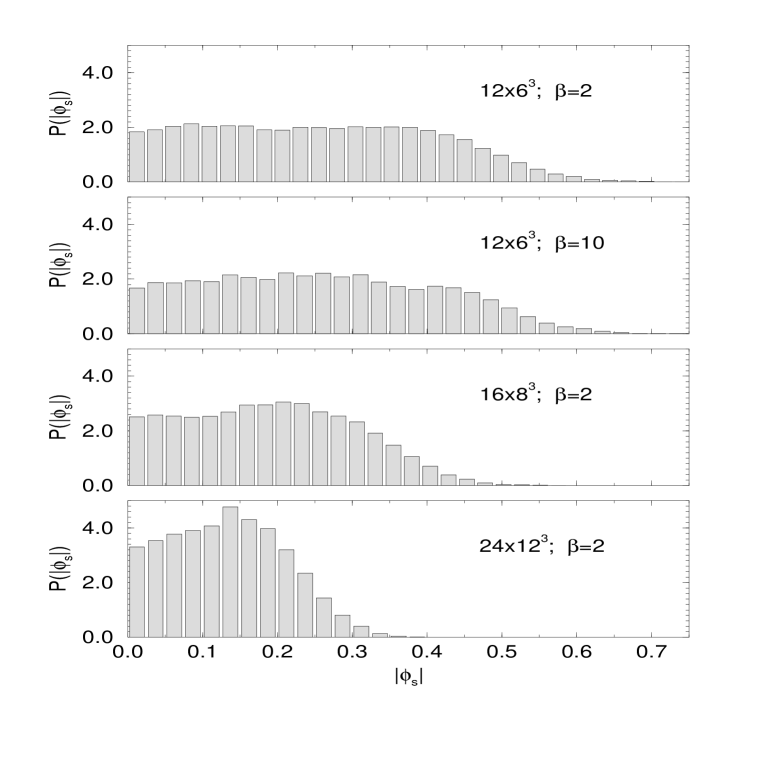
Figure 2: Distributions of the spacelike zero–momentum mode at different $\beta$–values and lattice sizes.

Figure 3: Free fermionic vector propagator (dashed line) and averaged constant-mode propagator (full line) for two $\beta$–values and lattice sizes $12\times 6^{3}$, $16\times 8^{3}$.

Figure 4: Effective masses corresponding to the fermion propagator results shown in Fig. 3.

Figure 5: Fermion mass as a function of inverse $\kappa$ obtained within the ZML gauge for $\beta=2.0$ on a $12\times 6^{3}$ lattice. The solid line represents a linear fit providing $~{}\kappa_{c}(\beta)=0.1307\pm 0.0001~{}$.

References

- [1] V.N. Gribov, Nucl. Phys. B139 (1978) 1.
- [2] T.P. Killingback, Phys. Lett.B138 (1984) 87.
- [3] K. Wilson, Phys. Rev. D10 (1974) 2445.
- [4] A. Nakamura and M. Plewnia, Phys. Lett. B255 (1991) 274.
- [5] A. Nakamura and R. Sinclair, Phys. Lett. B243 (1990) 396.
- [6] V.G. Bornyakov, V.K. Mitrjushkin, M. Müller-Preussker and F. Pahl, Phys. Lett. B317 (1993) 596.
- [7] Ph. de Forcrand and J.E. Hetrick, Nucl. Phys. (Proc. Suppl.) B42 (1995) 861.
- [8] I.L. Bogolubsky, V.K. Mitrjushkin, M. Müller-Preussker and P. Peter, Phys. Lett. B458 (1999) 102.
- [9] I.L. Bogolubsky, L. Del Debbio, V.K. Mitrjushkin, Phys. Lett. B463, 109 (1999).
- [10] V.K. Mitrjushkin, Phys. Lett. B389 (1996) 713.
- [11] V.K. Mitrjushkin, Phys. Lett. B390 (1997) 293.
- [12] D.B. Carpenter and C.F. Baillie, Nucl. Phys. B260 (1985) 103.
- [13] J.E. Mandula and M. Ogilvie, Phys. Lett. B248 (1990) 156.
- [14] D. Zwanziger, Nucl. Phys. B364 (1991) 127; B378 (1992) 525.
- [15] T.A. DeGrand and D. Toussaint, Phys. Rev. D22 (1980) 2478.
- [16] M. Göckeler, R. Horsley, P. Rakow, G. Schierholz and R. Sommer, Nucl. Phys. B371 (1992) 713.