1 Introduction

The center-vortex model of color confinement was proposed more than 20 years ago by ‘t Hooft [1] and other authors [2]. It was quite popular for a while, but then fell in oblivion, before being subjected to thorough tests in simulations of quantum chromodynamics on a lattice. One of the exceptions was the work of Tomboulis and collaborators [3]. In recent years the interest in this picture has been renewed due to our discovery of center dominance in SU(2) lattice gauge theory in maximal center gauge [4]. Substantial lattice evidence has then been accumulated on the role played by center vortices in color confinement [5, 6, 7].

Our procedure for identifying center vortices is based on center projection in maximal center gauge. This gauge brings each link variable as close as possible, on average, to a $Z_{N}$ center element, while preserving a residual $Z_{N}$ gauge invariance. Center projection then is a mapping of each SU($N$) link variable to the closest $Z_{N}$ center element.

The results that I would like to discuss here try to answer two questions related to our vortex-identification procedure:

1. How does the procedure work, why is it expected to locate center vortices relevant for confinement, and why does it in some cases fail, on lattice configurations preconditioned in a special way? (See Sec. 2 and more details in Ref. [8].)

2. A lot of numerical evidence favors the vortex-condensation theory in the SU(2) lattice gauge theory, but almost nothing has been done for SU(3). Does the mechanism work the same way for 3 colors instead of 2? (See Sec. 3 and Ref. [9].)

2 Vortex-Finding Property

2.1 Maximal Center Gauge in SU(2)

In SU(2) lattice gauge theory, the maximal center gauge is defined as a gauge in which the quantity

$${\cal{R}}[U]=\sum_{x}\sum_{\mu}\Bigl{|}\mbox{Tr}[U_{\mu}(x)]\Bigr{|}^{2}$$ (1)

reaches a maximum. It is worth noting that this gauge condition is equivalent to a Landau gauge-fixing condition on adjoint links, i.e.

$${\cal{R}}[U^{A}]=\sum_{x}\sum_{\mu}\mbox{Tr}[U^{A}_{\mu}(x)]$$ (2)

should be a maximum.

The simplest condition which a method for locating center vortices has to fulfill is to be able to find vortices inserted into a lattice configuration “by hand”. This will be called the “vortex-finding property”. Is this condition fulfilled when center vortices are located by our procedure of center projection in MCG?

One can argue for an affirmative answer in the following way: A center vortex is created, in a configuration $U$, by making a discontinuous gauge transformation. Call the result $U^{\prime}$. Apart from the vortex core, the corresponding link variables in the adjoint representation, $U^{A}$ and $U^{\prime A}$, are gauge equivalent. Let ${\cal R}[U^{A}]=\mbox{max}$ be a complete gauge-fixing condition (e.g. adjoint Landau gauge) on the adjoint links. Then (ignoring both Gribov copies and the core region) $U^{A}$ and $U^{\prime A}$ are mapped into the same gauge-fixed configuration $\tilde{U}^{A}$. The original fundamental link configurations $U$ and $U^{\prime}$ are thus transformed by the gauge-fixing procedure into configurations $\tilde{U},\ \tilde{U}^{\prime}$ which correspond to the same $\tilde{U}^{A}$. This means that $\tilde{U},\ \tilde{U}^{\prime}$ can differ only by continuous or discontinuous $Z_{2}$ gauge transformations, with the discontinuous transformation corresponding to the inserted center vortex in $U^{\prime}$. Upon center projection, $\tilde{U},\ \tilde{U}^{\prime}\rightarrow Z,\ Z^{\prime}$, and the projected configurations $Z,\ Z^{\prime}$ differ by the same discontinuous $Z_{2}$ transformation. The discontinuity shows up as an additional thin center vortex in $Z^{\prime}$, not present in $Z$, at the location of the vortex inserted by hand.

However, there are two caveats that could invalidate the argument:

1. We have neglected the vortex core region; and

2. Fixing to ${\cal R}[U^{A}]=\mbox{max}$ suffers from the existence of Gribov copies.

To find out whether these caveats are able to ruin the vortex-finding property, we have carried out a series of lattice tests. The simplest is the following:

1. Take a set of equilibrium SU(2) configurations.

2. From each configuration make three:

I – the original one;

II – the original one with $U_{4}(x,y,z,t)\rightarrow(-\mbox{1})\times U_{4}(x,y,z,t)$ for $t=t_{0}$, $x_{1}\leq x\leq x_{2}$ and all $y$, $z$, i.e. with 2 vortices (one lattice spacing thick) inserted by hand. Moreover, a random (but continuous) gauge transformation is performed on the configuration with inserted vortices;

III – a random copy of I.

3. Measure:

$$G(x)=\frac{\sum_{y,z}<P_{I}(x,y,z)P_{II}(x,y,z)>}{\sum_{y,z}<P_{I}(x,y,z)P_{III}(x,y,z)>}\;.$$ (3)

$P_{i}(x,y,z)$ is the Polyakov line measured on the configuration $i={}$I, II, or III.

If the method correctly identifies the inserted vortices, one expects

$$G(x)=\left\{\begin{array}[]{rl}-1&x\in[x_{1},x_{2}]\cr 1&\mbox{otherwise}\end{array}\right.\;.$$ (4)

(a) Configurations fixed directly to the maximal center gauge.

(b) Configurations first fixed to the Landau gauge, then to MCG.

Figure 1.  : Graph of $G(x)$ for configurations with thin inserted vortices ($14^{3}\times 12$ lattice). The discontinuity was inserted to the time links within the volume $4\!\leq\!x\!\leq\!10,\;0\!\leq\!y\!<\!14,\;0\!\leq\!z\!<\!14$ at the time slice $t=T$.

The result of the test is shown in Fig. 1(a). The inserted vortices are clearly recognized, and the associated Dirac volume is found in its correct location. The vortex-finding property is also preserved when we insert vortices with a core a few lattice spacings thick.

2.2 MCG Preconditioned with Landau Gauge

It has been shown recently by Kovács and Tomboulis [10] that if one first fixes to Landau gauge (LG), before relaxation to maximal center gauge, center dominance is lost. They argued that this problem casts some doubt on the physicality of objects defined through center projection in MCG.

This failure has a simple explanation: LG preconditioning destroys the vortex-finding property. This is illustrated by redoing the test shown in Fig. 1(a), only with a prior fixing to Landau gauge. The result, shown in Fig. 1(b), is that the vortex-finding condition is not satisfied; the Dirac volume is not reliably identified.

The Gribov copy problem, which is fairly harmless on most of the gauge orbit [5], seems severe enough to ruin vortex-finding on a tiny region of the gauge orbit near Landau gauge.

2.3 Other Gauges

The vortex-finding argument above does not seem to single out MCG. In fact, there should exist (infinitely) many gauges with the vortex-finding property. They should fulfill the following requirements:

1. The gauge condition depends only on the adjoint representation links.

2. It is a complete gauge-fixing for adjoint link variables.

3. The gauge fixing transforms most links to be close to center elements, at weak coupling.

We have tried a couple of gauge conditions, and the results are summarized in Table 1. It turns out in all cases that the loss of the vortex-finding property goes hand in hand with the loss of center dominance. A notable fact is that the recently proposed Laplacian center gauge [11], which is free of the Gribov-copy problem, is a perfect (thin-)vortex finder, i.e. the simple expectation (4) is satisfied by the numerical data exactly.

TABLE 1.  : Comparison of various adjoint gauges. (Details see in Ref. [9].)

 Gauge Center dominance Vortex-finding property  maximal center gauge yes yes Landau gauge, then MCG no no asymmetric adjoint gauge yes yes adjoint Coulomb gauge no no “modulus” Landau gauge no no MCG, then “modulus” Landau gauge yes yes Laplacian center gauge yes perfect!  

3 Evidence for Center Dominance in SU(3) Lattice Gauge Theory

3.1 Maximal Center Gauge in SU(3)

The maximal center gauge in SU(3) gauge theory is defined as the gauge which brings link variables $U$ as close as possible to elements of its center $Z_{3}$. This can be achieved as in SU(2) by maximizing a “mesonic” quantity

$${\cal{R}}=\sum_{x}\sum_{\mu}\Bigl{|}\mbox{Tr}[U_{\mu}(x)]\Bigr{|}^{2},$$ (5)

or, alternatively, a “baryonic” one

$${\cal{R}}^{\prime}=\sum_{x}\sum_{\mu}\mbox{Re}\left(\left[\mbox{Tr}\;U_{\mu}(x)\right]^{3}\right).$$ (6)

The latter was the choice of Ref. [5], where we used the method of simulated annealing for iterative maximization procedure. The convergence to the maximum was rather slow and forced us to restrict simulations to small lattices and strong couplings.

The results, that will be presented below, were obtained in a gauge defined by the “mesonic” condition (5). The maximization procedure for this case is inspired by the Cabibbo–Marinari–Okawa SU(3) heat bath method [12]. The idea of the method is as follows: In the maximization procedure we update link variables to locally maximize the quantity (5) with respect to a chosen link. Instead of trying to find the optimal gauge-transformation matrix $\Omega(x)$, we take an SU(2) matrix $g(x)$ and embed it into one of the three diagonal SU(2) subgroups of SU(3). The expression for a chosen link is then maximized with respect to $g$, with the constraint of $g$ being an SU(2) matrix. This reduces to an algebraic problem (plus a solution of a non-linear equation). Once we obtain the matrix $g(x)$, we update link variables touching the site $x$, and repeat the procedure for all three subgroups of SU(3) and for all lattice sites. This constitutes one center gauge fixing sweep. Center projection is then done by replacing each link matrix by the closest element of $Z_{3}$.

The above iterative procedure was independently developed by Montero. Its detailed description is contained in his recent publication [13].

3.2 Center Dominance in SU(3) Lattice Gauge Theory

The effect of creating a center vortex linked to a given Wilson loop in SU(3) lattice gauge theory is to multiply the Wilson loop by an element of the gauge group center, i.e. $W(C)\rightarrow e^{\pm 2\pi i/3}W(C)$. Quantum fluctuations in the number of vortices linked to a Wilson loop can be shown to lead to its area law falloff; the simplest, but urgent question is whether center disorder is sufficient to produce the whole asymptotic string tension of full, unprojected lattice configurations.

We have computed Wilson loops and Creutz ratios at various values of the coupling $\beta$ on a $12^{4}$ lattice, from full lattice configurations, center-projected link configurations in maximal center gauge, and also from configurations with all vortices removed. Figure 2(a) shows a typical plot at $\beta=5.6$. It is obvious that center elements themselves produce a value of the string tension which is close to the asymptotic value of the full theory. On the other hand, if center elements are factored out from link matrices and Wilson loops are computed from SU(3)/$Z_{3}$ elements only, the Creutz ratios tend to zero for sufficiently large loops. The errorbars are, however, rather large, and one cannot draw an unambiguous conclusion from the data.

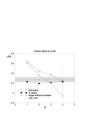
(a) Creutz ratios for the original, the $Z_{3}$ projected, and the modified (with vortices removed) ensembles. The value of $\chi(4)$ (shown in grey) comes from the compilation of Levi [14].

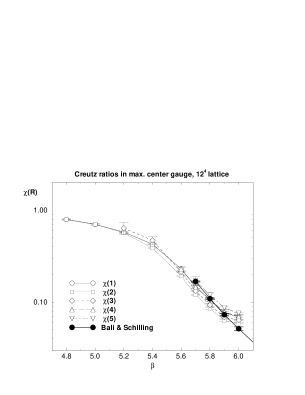
(b) Center-projected Creutz ratios vs. $\beta$. Full circles connected with a solid line are asymptotic values quoted by Bali and Schilling [17].

Figure 2.  : Creutz ratios in SU(3) lattice gauge theory.

Center dominance by itself does not prove the role of center degrees of freedom in QCD dynamics [15, 16]; some sort of center dominance exists also without any gauge fixing and can hardly by attributed to center vortices. Distinctive features of center-projected configurations in maximal center gauge in SU(2), besides center dominance, were that:

1. Creutz ratios were approximately constant starting from small distances (this we called “precocious linearity”),

2. the vortex density scaled with $\beta$ exactly as expected for a physical quantity with dimensions of inverse area.

Precocious linearity, the absence of the Coulomb part of the potential on the center-projected lattice at short distances, can be quite clearly seen from Fig. 2(a). One observes some decrease of the Creutz ratios at intermediate distances. A similar effect is present also at other values of $\beta$. It is not clear to us whether this decrease is of any physical relevance, or whether it should be attributed to imperfect fixing to the maximal center gauge.

The issue of scaling is addressed in Figure 2(b). Here values of various Creutz ratios are shown as a function of $\beta$ and compared to those quoted in Ref. [17]. All values for a given $\beta$ lie close to each other and are in reasonable agreement with asymptotic values obtained in time-consuming SU(3) pure gauge theory simulations. The plot in Fig. 2(b) is at the same time a hint that the P-vortex density also scales properly. The density is approximately proportional to the value of $\chi(1)$ in center-projected configurations, and $\chi(1)$ follows the same scaling curve as Creutz ratios obtained from larger Wilson loops.

A closer look at Fig.  2(b) reveals that there is no perfect scaling, similar to the SU(2) case, in our SU(3) data. Broken lines connecting the data points tend to bend at higher values of $\beta$. In our opinion, this is a finite-volume effect and should disappear for larger lattices.

4 Conclusions

I conclude with the following comments/conclusions:

1. Center vortices are created by discontinuous gauge transformations, which make no reference to any particular gauge condition. However, appropriate gauge fixing is necessary to reveal relevant center vortices: In MCG – and in an infinite class of other adjoint gauges – such discontinuous transformations are squeezed to the identity everywhere except on Dirac volumes, whose locations (together with those of the associated vortices) are then revealed upon center projection.

2. If the vortex-finding property is destroyed by some modification of the gauge-fixing and center-projection procedure, then center vortices are not correctly identified on thermalized lattices, and center dominance in the projected configurations is lost. This fact does not call into question the physical relevance of P-vortices found by our usual procedure (which has the vortex-finding property); that relevance is implied by the strong correlation that was shown to exist between these objects and gauge-invariant observables.

3. Center dominance is quite clearly seen also in SU(3) lattice gauge theory, however, more convincing data and better gauge-fixing procedure is needed.

Acknowledgements
I am grateful to the organizers of this excellent Workshop, especially Valja Mitrjushkin, for invitation and warm hospitality.

References

- [1] ’t Hooft, G. (1978) On the phase transition towards permanent quark confinement, Nuclear Physics B138, 1.
-
[2]
Vinciarelli, P. (1978)
Fluxon solutions in nonabelian gauge models,
Physics Letters 78B, 485;
Yoneya, T. (1978) topological excitations in Yang–Mills theories: Duality and confinement, Nuclear Physics B144, 195;
Cornwall, J.M. (1979) Quark confinement and vortices in massive gauge invariant QCD, Nuclear Physics B157, 392;
Nielsen, H.B., and Olesen, P. (1979) A quantum liquid model for the QCD vacuum: Gauge and rotational invariance of domained and quantized homogeneous color fields, Nuclear Physics B160, 380;
Mack, G. (1980) Properties of lattice gauge theory models at low temperatures, in G. ’t Hooft et al. (eds.), Recent Developments in Gauge Theories, Plenum Press, New York, p. 0217;
Feynman, R.P. (1981) The qualitative behavior of Yang–Mills theory in (2+1)-dimensions, Nuclear Physics B188, 479. - [3] Tomboulis, E.T. (1999) Talk at this Workshop, see these Proceedings, and references therein.
- [4] Del Debbio, L., Faber, M., Greensite, J., and Olejník, Š. (1997) Center dominance and vortices in SU(2) lattice gauge theory, Physical Review D55, 2298 [hep-lat/9610005].
- [5] Del Debbio, L., Faber, M., Giedt, J., Greensite, J., and Olejník, Š. (1998) Detection of center vortices in the lattice Yang–Mills vacuum, Physical Review D58, 094501 [hep-lat/9801027].
- [6] Langfeld, K., Reinhardt, H., and Tennert, O. (1998) Confinement and scaling of the vortex vacuum of SU(2) lattice gauge theory, Physics Letters B419, 317 [hep-lat/9710068].
- [7] de Forcrand, Ph., and D’Elia, M. (1999) Relevance of center vortices to QCD, Physical Review Letters 82, 4582 [hep-lat/9901020].
- [8] Faber, M., Greensite, J., Olejník, Š., and Yamada, D. (1999) The vortex-finding property of maximal center (and other) gauges, hep-lat/9910033.
- [9] Faber, M., Greensite, J., and Olejník, Š. (1999) First evidence for center dominance in SU(3) lattice gauge theory, hep-lat/9911006.
- [10] Kovács, T., and Tomboulis, E.T. (1999) P-vortices and the Gribov problem, Physics Letters B463, 104 [hep-lat/9905029].
-
[11]
Alexandrou, C., D’Elia, M., and de Forcrand, Ph. (1999)
The relevance of center vortices,
hep-lat/9907028;
Alexandrou, C., de Forcrand, Ph., and D’Elia, M. (1999) The role of center vortices in QCD, hep-lat/9909005. -
[12]
Cabibbo, N., and Marinari, E. (1982)
A new method for updating SU() matrices in computer simulations
of gauge theories,
Physics Letters B119, 387;
Okawa, M. (1982) Monte Carlo study of the Eguchi–Kawai model, Physical Review Letters 49, 353. - [13] Montero, Á. (1999) Study of SU(3) vortex-like configurations with a new maximal center gauge fixing method, Physics Letters B467, 106 [hep-lat/9906010].
- [14] Levi, A.R. (n.d.) Lattice QCD Results with a Java Applet, available on the World Wide Web at http://physics.bu.edu/leviar/res.html.
- [15] Ambjørn, J., and Greensite, J. (1998) Center disorder in the 3D Georgi-Glashow model, Journal of High Energy Physics 9805, 004 [hep-lat/9804022].
- [16] Faber, M., Greensite, J., and Olejník, Š. (1999) Center projection with and without gauge fixing, Journal of High Energy Physics 9901, 008 [hep-lat/9810008].
- [17] Bali, G., and Schilling, K. (1993) Running coupling and the parameter from SU(3) lattice simulations, Physical Review D47, 661 [hep-lat/9208028].