Renormalization group flow of SU(3) lattice gauge theory
- Numerical studies in a two coupling space -

Abstract

We investigate the renormalization group (RG) flow of SU(3) lattice gauge theory in a two coupling space with couplings $\beta_{11}$ and $\beta_{12}$ corresponding to $1\times 1$ and $1\times 2$ loops respectively. Extensive numerical calculations of the RG flow are made in the fourth quadrant of this coupling space, i.e., $\beta_{11}>0$ and $\beta_{12}<0$. Swendsen’s factor two blocking and the Schwinger-Dyson method are used to find an effective action for the blocked gauge field. The resulting renormalization group flow runs quickly towards an attractive stream which has an approximate line shape. This is a numerical evidence of a renormalized trajectory which locates close to the two coupling space. A model flow equation which incorporates a marginal coupling (asymptotic scaling term), an irrelevant coupling and a non-perturbative attraction towards the strong coupling limit reproduces qualitatively the observed features. We further examine the scaling properties of an action which is closer to the attractive stream than the currently used improved actions. It is found that this action shows excellent restoration of rotational symmetry even for coarse lattices with $a\sim 0.3$ fm.

1 Introduction

Since Wilson’s first numerical renormalization group (RG) analysis of SU(2) gauge theory [1], there have been many Monte Carlo RG studies of non-perturbative $\beta$-functions (see Ref.[2] and references therein). In these analysis indirect information about the $\beta$ function, such as $\Delta\beta$, has been obtained [3]. Recent progress of lattice techniques [4, 5, 6] allows us to estimate directly the RG flow in multi-coupling space [7].

We study renormalization effects by means of a blocking transformation which changes the lattice cut-off but leaves the long range contents of the system invariant. A new blocked action $S^{\prime}$ as a function of blocked link variables $V$’s is constructed from the original action $S(U)$ as

$$e^{-S^{\prime}(V)}=\int{\cal D}Ue^{-S(U)}\delta(V-P(U)),$$ (1)

where $P$ defines the blocking transformation. The action $S^{\prime}$ includes the renormalization effects induced by blocking. In the space of coupling constants, the blocking transformation makes a transition from a point corresponding to $S$ to a new point, $S^{\prime}$. Repeating the blocking transformation, we obtain trajectories in coupling space which define the so called renormalization group flow.

There is a special trajectory, i.e. renormalized trajectory (RT), which starts at the ultra-violet fixed point. On the RT, the long range information corresponding to continuum physics is preserved. Recently Hasenfratz and Niedermayer have stressed that the action on the RT can indeed be considered as a “perfect action” [9]. Therefore if we find a RT corresponding to a blocking transformation, it provides an action which gives accurate results corresponding to the continuum limit. Even if it is an approximate one, it serves as a well-improved action. In this sense, a pioneering work has been done by Iwasaki more than ten years ago [8]. He estimated a RT by matching Wilson loops based on a perturbative approximation, and proposed an improved action which we will call below Iwasaki action.

In this work, we analyze numerically the RG flow in two coupling space, $(\beta_{11},\beta_{12})$, of SU(3) lattice gauge theory and clarify the structure of the renormalization group flow. The action is restricted to the following form;

$$S = \beta_{11}\sum_{{\rm plaq}}(1-{1\over 3}{\rm Re\mbox{Tr}}P_{{\rm plaq}})+\beta_{12}\sum_{{\rm rect}}(1-{1\over 3}{\rm Re\mbox{Tr}}P_{{\rm rect}})$$

Here $P_{{\rm plaq}}$ and $P_{{\rm rect}}$ correspond to $1\times 1$ and $1\times 2$ loops, respectively.

The main purpose of the present work is to perform an extensive study of the RT beyond a perturbative analysis. It is a non-trivial fact whether the RT locates near the two coupling space, i.e. in the $(\beta_{11},\beta_{12})$ plane. If no remnant of the RT can be seen in this plane, the two coupling space is insufficient to obtain good improved actions. In this sense, a global analysis of the RG flow from weak to strong coupling regions is indispensable. Parts of our analysis were reported in Refs.[10, 17], and in this paper we present much more data which are enough to confirm the existence of RT.

Our analysis is performed in the fourth quadrant of the coupling space. We examine renormalization effects induced by Swendsen’s factor two blocking on the plaquette action as well as on some improved actions. In addition, we try to clarify the global structure of the RG flow. An evidence that the RT sits close to the two coupling space is provided by the fact that the flow runs quickly towards a narrow attractive stream. Characteristic features of the flow in the strong and weak coupling regions are also found. The observed features are reproduced by a model flow equation which incorporates a marginal coupling (asymptotic scaling term), an irrelevant coupling and a non-perturbative attraction towards the strong coupling limit.

Based on the flow structure, we examine the scaling properties of several actions defined in this two coupling space. Tests are made for the rotational invariance and the scaling of $\sqrt{\sigma}/T_{c}$. Near the attractive stream, we find good restoration of the rotational invariance.

This paper is organized as follows. In sect. 2, the basic tools for the analysis are given. Sect. 3 is devoted to present simulations and numerical results of the RG flow. Scaling tests are described in sect. 4. In sect. 5, a model flow equation which can reproduce the observed RG flow is proposed. Renormalization effects beyond the two coupling space are discussed in sect. 6. A summary of results is given in sect. 7.

2 Blocking transformation and determination of renormalization effects

Here we describe the basic framework to study the RG flow for SU(3) gauge fields on the lattice. First we produce field configurations with an action $S$ which has coupling constants $(\beta_{11},\beta_{12},\cdots)$, and apply a blocking transformation on these configurations. Next we determine an action $S^{\prime}$ with coupling constants $(\beta^{\prime}_{11},\beta^{\prime}_{12},\cdots)$ which reproduces the transformed configurations. In this way, we extract a flow in the coupling constant space from the original coupling constants $\{\beta\}$ to the transformed ones $\{\beta^{\prime}\}$; this is the RG flow.

In order to perform the blocking transformation on a lattice, we adopt Swendsen’s factor-two blocking [11]. For a set of SU(3) link variables $U_{\mu}(n)$, a blocked field is constructed as:

$$Q_{\mu}(n)=U_{\mu}(n)U_{\mu}(n+\hat{\mu})+c\sum_{\nu\neq\mu}U_{\nu}(n)U_{\mu}(n+\hat{\nu})U_{\mu}(n+\hat{\nu}+\hat{\mu})U_{-\nu}(n+\hat{\nu}+2\hat{\mu}).$$ (3)

Here $c$ is a parameter to control the weight of the staple-like paths. A convenient notation $V_{-\mu}(n)=V_{\mu}^{\dagger}(n-\hat{\mu})$ is also used and the sum is taken over negative as well as positive direction. $Q_{\mu}(n)$ is projected onto the blocked SU(3) gauge field $V_{\mu}(n)$ by maximizing ${\rm Re}{\rm\mbox{Tr}}(Q_{\mu}(n){V}_{\mu}^{{\dagger}}(n))$.

To determine the effective action $S^{\prime}$ on blocked configuration $V$, we use the Schwinger-Dyson method [4]. This is based on the following identity: for a link $V_{l_{0}}$, consider the quantities

$$\langle\mbox{Im}\mbox{Tr}(\lambda^{b}V_{l_{0}}G_{l_{0}}^{\alpha})\rangle=\frac{1}{Z}\int{\cal D}V\mbox{ Im \mbox{Tr} }(\lambda^{b}V_{l_{0}}G_{l_{0}}^{\alpha})\ e^{-S^{\prime}}$$ (4)

where $\lambda^{b}$ stands for Gell-Mann matrices. Here action is assumed to have the form,

$$S^{\prime}=\sum_{l}~{}\sum_{\gamma}{\beta_{\gamma}^{\prime}\over 2}[1-{1\over 3}{\rm Re}~{}{\rm\mbox{Tr}}V_{l}G_{l}^{\gamma}]$$ (5)

and $G_{l}^{\gamma}$ stands for a “staple” coupling to the link $l$ in a loop of type $\gamma$. For the present analysis, $\gamma$ corresponds to a plaquette and a rectangle. Eq. (4) should be invariant under the change of variable $V_{l_{0}}\rightarrow(1+i\epsilon\lambda^{b})V_{l_{0}}$. Setting terms linear in $\epsilon$ to be zero, we get the identity,

$$\int{\cal D}V[{\rm Re}{\rm\mbox{Tr}}((\lambda^{b})^{2}V_{l_{0}}G_{l_{0}}^{\alpha})+{\rm Im}{\rm\mbox{Tr}}(\lambda^{b}V_{l_{0}}G_{l_{0}}^{\alpha}){\rm Im}{\rm\mbox{Tr}}(\lambda^{b}V_{l_{0}}G_{l_{0}})]\ e^{-S^{\prime}}=0,$$ (6)

where

$$G_{l}=\sum_{\gamma}\frac{\beta_{\gamma}^{\prime}}{6}G_{l}^{\gamma}.$$ (7)

Summing over $b$ in the expression (6) above, we obtain the Schwinger-Dyson equation,

$${8\over 3}{\rm Re}\langle{\rm\mbox{Tr}}(V_{l_{0}}G_{l_{0}}^{\alpha})\rangle=\sum_{\gamma}{\beta_{\gamma}^{\prime}\over 6}\{-{\rm Re}\langle{\rm\mbox{Tr}}(V_{l_{0}}G_{l_{0}}^{\alpha}V_{l_{0}}G_{l_{0}}^{\gamma})\rangle$$

$$+{\rm Re}\langle{\rm\mbox{Tr}}(G_{l_{0}}^{\alpha}(G_{l_{0}}^{\gamma})^{\dagger})\rangle-{2\over 3}\langle{\rm Im~{}\mbox{Tr}}(V_{l_{0}}G_{l_{0}}^{\alpha}){\rm Im~{}\mbox{Tr}}(V_{l_{0}}G_{l_{0}}^{\gamma})\rangle\}.$$ (8)

Here we have used the identity: $\sum_{b=1}^{8}{\rm\mbox{Tr}}(\lambda^{b}A){\rm\mbox{Tr}}(\lambda^{b}B)=2{\rm\mbox{Tr}}AB-\frac{2}{3}{\rm\mbox{Tr}}A{\rm\mbox{Tr}}B.$ We apply eq. (8) to the blocked configurations, and calculate the expectation values $\langle\cdots\rangle$ on both sides. Now eq. (8) may be considered as a set of linear equations with $\beta_{\gamma}$’s as unknowns. It is noted that we may use other loop operators instead of $G^{\alpha}$. However a minimal choice is to take the same $G^{\alpha}$s as the ones entering the action. In this case, the number of equations is equal to the number of unknown couplings.

It is noted that the canonical Demon method also works for the present purpose [6]. This method tunes the effective action so as to reproduce the mean values of the plaquette and rectangular loops whereas the Schwinger-Dyson method respects wider loops which are combination of staples such as ${\rm\mbox{Tr}}(G_{l}^{\alpha}(G_{l}^{\gamma})^{\dagger})$. In case of a limited coupling space, they may lead to different actions. Because the systematic errors involved in both methods are not known in the present stage, only the results obtained via the Schwinger-Dyson method are presented in this work.

Since we study the RG flow in the two coupling space, we show corresponding Schwinger-Dyson equation explicitly.

$$\left(\begin{array}[]{l}\beta^{\prime}_{11}\\ \beta^{\prime}_{12}\end{array}\right)=\left(\begin{array}[]{ll}A_{11}&A_{12}\\ A_{21}&A_{22}\end{array}\right)^{-1}\left(\begin{array}[]{l}\langle\mbox{Re Tr}(P^{(1)}_{\mu\nu})\rangle\\ \langle\mbox{Re Tr}(P^{(2)}_{\mu\nu})\rangle\end{array}\right)$$ (15)

where

$$\begin{array}[]{l}A_{11}={1\over 16}\sum_{\sigma\neq\mu}{\rm Re}[\langle\mbox{Tr}(P^{(1)}_{\mu\nu}P^{(1)\dagger}_{\mu\sigma})\rangle-\langle\mbox{Tr}(P^{(1)}_{\mu\nu}P^{(1)}_{\mu\sigma})\rangle-{1\over 3}\langle\mbox{Tr}(P^{(1)}_{\mu\nu})\mbox{Tr}(P^{(1)\dagger}_{\mu\sigma}-P^{(1)}_{\mu\sigma})\rangle]\\ A_{12}={1\over 16}\sum_{\sigma\neq\mu}{\rm Re}[\langle\mbox{Tr}(P^{(1)}_{\mu\nu}P^{(2)\dagger}_{\mu\sigma})\rangle-\langle\mbox{Tr}(P^{(1)}_{\mu\nu}P^{(2)}_{\mu\sigma})\rangle-{1\over 3}\langle\mbox{Tr}(P^{(1)}_{\mu\nu})\mbox{Tr}(P^{(2)\dagger}_{\mu\sigma}-P^{(2)}_{\mu\sigma})\rangle\\ \hskip 93.89409pt+\langle\mbox{Tr}(P^{(1)}_{\mu\nu}P^{H\dagger}_{\mu\sigma})\rangle-\langle\mbox{Tr}(P^{(1)}_{\mu\nu}P^{H}_{\mu\sigma})\rangle-{1\over 3}\langle\mbox{Tr}(P^{(1)}_{\mu\nu})\mbox{Tr}(P^{H\dagger}_{\mu\sigma}-P^{H}_{\mu\sigma})\rangle]\\ A_{21}={1\over 16}\sum_{\sigma\neq\mu}{\rm Re}[\langle\mbox{Tr}(P^{(2)}_{\mu\nu}P^{(1)\dagger}_{\mu\sigma})\rangle-\langle\mbox{Tr}(P^{(2)}_{\mu\nu}P^{(1)}_{\mu\sigma})\rangle-{1\over 3}\langle\mbox{Tr}(P^{(2)}_{\mu\nu})\mbox{Tr}(P^{(1)\dagger}_{\mu\sigma}-P^{(1)}_{\mu\sigma})\rangle]\\ A_{22}={1\over 16}\sum_{\sigma\neq\mu}{\rm Re}[\langle\mbox{Tr}(P^{(2)}_{\mu\nu}P^{(2)\dagger}_{\mu\sigma})\rangle-\langle\mbox{Tr}(P^{(2)}_{\mu\nu}P^{(2)}_{\mu\sigma})\rangle-{1\over 3}\langle\mbox{Tr}(P^{(2)}_{\mu\nu}){\rm Tr}(P^{(2)\dagger}_{\mu\sigma}-P^{(2)}_{\mu\sigma})\rangle\\ \hskip 93.89409pt+\langle\mbox{Tr}(P^{(2)}_{\mu\nu}P^{H\dagger}_{\mu\sigma})\rangle-\langle\mbox{Tr}(P^{(2)}_{\mu\nu}P^{H}_{\mu\sigma})\rangle-{1\over 3}\langle\mbox{Tr}(P^{(2)}_{\mu\nu}){\rm Tr}(P^{H\dagger}_{\mu\sigma}-P^{H}_{\mu\sigma})\rangle]\end{array}$$ (22)

with

$$\begin{array}[]{ll}P^{(1)}_{\mu\nu}(n)=&V_{\mu}(n)V_{\nu}(n+\mu)V_{-\mu}(n+\mu+\nu)V_{-\nu}(n+\nu)\\ P^{(2)}_{\mu\nu}(n)=&V_{\mu}(n)V_{\nu}(n+\mu)V_{\nu}(n+\mu+\nu)V_{-\mu}(n+\mu+2\nu)V_{-\nu}(n+2\nu)V_{-\nu}(n+\nu)\\ P^{H}_{\mu\nu}(n)=&V_{\mu}(n)[V_{\nu}(n+\mu)V_{-\mu}(n+\mu+\nu)V_{-\mu}(n+\nu)V_{-\nu}(n-\mu+\nu)V_{\mu}(n-\mu)\\ &+V_{\mu}(n+\mu)V_{\nu}(n+2\mu)V_{-\mu}(n+2\mu+\nu)V_{-\mu}(n+\mu+\nu)V_{-\nu}(n+\nu)]\ \ .\end{array}$$ (27)

3 Simulation and numerical results of the RG flow

Using the techniques in the previous section, we study the coupling flow induced by the factor two blocking. We set the blocking parameter $c=0.5$.

Series of simulations on lattices of size $8^{4}$ and $16^{4}$ are performed. The region surveyed in the present work is the fourth quadrant of the $(\beta_{11},\beta_{12})$ plane which covers most improved actions presently known. We use the pseudo heat-bath method to generate the gauge fields. The blocking transformation is carried out at more than 30 points. At each point, about 100 configurations separated by every 100 sweeps are used to determine the renormalized couplings $\beta_{11}^{\prime}$ and $\beta_{12}^{\prime}$ through the Schwinger-Dyson method. Examples in the determination of the coupling are shown in Table 1 and 2. The errors are given by the Jack-knife method and they are relatively small even at deconfined points. Analyses are made also for data samples in which configurations are separated by 1000 sweeps. Those data agree with that of the standard samples within error bars. An example is shown in the last two lines of Table 1.

$\beta_{11}$	$\beta_{12}$	$\beta_{11}^{\prime}$	$\beta_{12}^{\prime}$
7.00	0.0	13.188(22)	-1.6564(94)
7.00	-0.35	8.148(29)	-1.0431(98)
11.00	-0.9981	15.189(73)	-2.329(19)
13.20	-1.493	15.445(50)	-2.559(15)
(${\dagger}$)13.20	-1.493	15.519(37)	-2.583(13)

Table 1: Examples of renormalized couplings $\beta_{11}^{\prime}$ and $\beta_{12}^{\prime}$ obtained through the Schwinger-Dyson method. A hundred configurations are used at each point. For (${\dagger}$) , measurements are performed every 1000 pseudo heat-bath steps, while for the rest of the data we measure every 100 steps.

We check also the effect of the finite temperature phase transition on the determination of the coupling constants. Since the blocking transformation induces renormalization effects corresponding to a change of lattice cutoff, the resulting coupling shifts are insensitive to the phases. We examine this point by comparing results belonging to the confined phase on the $16^{4}$ lattice while remaining deconfined on the $8^{4}$ lattice at several values of $\beta$ as shown in Table 2. The finite temperature phase transition on the $8^{4}$ and $16^{4}$ lattices for the plaquette action takes place at approximately $\beta_{11}=5.9$ and $6.3$ which roughly correspond to $a\sqrt{\sigma}=0.27$ and $a\sqrt{\sigma}=0.14$ respectively. As seen in Table 2, both results agree within errors.

$\beta_{11}$	$\beta_{12}$	$\beta_{11}^{\prime}$	$\beta_{12}^{\prime}$	lattice size
6.20	0.0	9.515(56)	-1.156(23)	$8^{4}$ deconfined
		9.547(14)	-1.1671(53)	$16^{4}$ confined
9.8496	-0.8937	12.368(61)	-1.883(16)	$8^{4}$ deconfined
		12.280(14)	-1.8688(41)	$16^{4}$ confined
9.0	-1.03332	7.211(38)	-1.046(17)	$8^{4}$ deconfined
		7.2086(86)	-1.0456(30)	$16^{4}$ confined

Table 2: Renormalized couplings $\beta^{\prime}_{11}$ and $\beta^{\prime}_{12}$ on the deconfined and confined lattices. These are calculated with 50 configurations, and measurements are performed every 100 steps.

Our results are summarized in Fig. 1, in which the coupling shift resulting after the blocking is indicated by arrows.

Figure 1: Renormalization group flow of SU(3) lattice gauge theory in the two coupling space $(\beta_{11},\beta_{12})$. There is an attractive stream to which the arrows converge. Dotted and dashed lines correspond to ( tree level ) Symanzik action and Iwasaki action respectively. The long dashed line corresponds to the “DBW2” action introduced in section 4. On the DBW2 line, the black dot is the point reached by twice blocking from the plaquette action at $\beta=6.3$ on a $32^{3}\times 64$ lattice [17].

As shown in the figure, several characteristics of the flow are seen. If we start from the plaquette action ($\beta_{12}=0$ line), renormalization results in a negative $\beta_{12}$ as expected by a perturbative analysis. At $\beta_{11}=6\sim 8$, the renormalization effect is very strong making $\beta_{11}$ twice larger and $\beta_{12}$ negative. The resulting points are far below the line of the tree-level Symanzik action. On the other hand, in the strong coupling region below $\beta_{11}<5$, the effect of the renormalization is to reduce $\beta_{11}$. Therefore, the plaquette action suffers large renormalization effects and it is far from the renormalized trajectory.

Points starting on the line defined by the tree-level Symanzik action, $\beta_{12}/\beta_{11}=-0.05$, are RG transformed onto ones with $\beta_{12}$ far more negative. Although renormalization effects are reduced, the trend is the same as that of the plaquette action. This means that tree-level Symanzik action is still far from blocking invariant. This indicates that perturbative $O(a^{2})$ improvement is insufficient at least for the currently used range of lattice spacings.

Now we look at flows starting from points on the line corresponding to Iwasaki action, i.e., $\beta_{12}=-0.09073\beta_{11}$. We see that renormalization occurs approximately along the line up to an intermediate point ($\beta_{11}\approx 7.3,\beta_{12}=-0.09073\beta_{11}$). At larger $\beta_{11}$, however, flows depart from the line defined by this action. Thus the present blocking transformation renormalizes Iwasaki action further and induces more negative values of $\beta_{12}$ above the intermediate coupling region.

Let us turn to the global structure of the flow. Blockings are made starting from points with $\beta_{12}/\beta_{11}=-0.1\sim-0.15$. For those points, the renormalization effect is relatively small and converges to a narrow stream. This trend is manifest at strong coupling. As a whole, there is an attractive stream which the flow approaches quickly. Furthermore, once the flow reaches the stream, it runs along it. Therefore actions on the attractive stream are approximately blocking invariant apart from a normalization. The shape of the attractive stream is clearly recognized as a parabolic curve in the strong coupling region while at points far from the origin, it is less obvious with the present data. This is a remarkable indication that the renormalized trajectory locates close to the $(\beta_{11},\beta_{12})$ coupling space. This is an encouraging result for finding a good improved action in this two coupling space.

A closer look at the attractive flow allows to extract more information. If we start from the Wilson action at $\beta_{11}>6.0$, the first blocking leads to larger renormalization effects as $\beta_{11}$ increases and the resulting flow vectors have the same direction pointing towards increasing $\beta_{11}$ further until the flow has reached the main attractive stream. This feature seems consistent with a flow induced by an irrelevant coupling. In the strong coupling region the behavior is quite different, under the blocking the coupling moves deeper into strong coupling, with the main stream following a parabolic behavior, as already indicated above. In section 5, we will try to reproduce these features by a model equation including an irrelevant coupling, an asymptotic scaling term and a driving term derived from the area law behavior of Wilson loops.

4 Tests of improvement for actions near the attractive stream

The purpose of this section is to examine the degree of improvement for actions lying near the attractive stream. As shown in Fig. 1, we expect that the irrelevant coupling is considerably reduced and actions will be dominated by the marginal coupling term. Here we analyze an action suggested by double blocking from Wilson action at $\beta=6.3$ on a $32^{3}\times 64$ lattice where ($\beta_{11},\beta_{12})=(7.986(13),-0.09169(41))$ has been obtained [17]. This action is called DBW2 (doubly blocked from Wilson action in two coupling space ) and has a value of $\beta_{12}/\beta_{11}$ equal to -0.1148 (long dashed line in Fig. 1).

There are many ways to test improvement. Among them, we will examine rotational invariance of the heavy quark potential and independence of $T_{c}/\sqrt{\sigma}$ on the lattice spacing. Let us define a measure of violation of rotational symmetry as

$$\delta_{V}^{2}=\sum_{{\rm off}}{[V(R)-V_{{\rm on}}(R)]^{2}\over V(R)^{2}\delta V(R)^{2}}/(\sum_{{\rm off}}{1\over\delta V(R)^{2}})$$ (28)

where $V(R)$ is the static quark potential and $\delta V(R)$ is its error. $V_{\rm on}(R)$ is a fitting function to only on-axis data. $\sum_{{\rm off}}$ means summations over off-axis data. This quantity is measured on the configurations generated by the DBW2 action. For comparison, plaquette-, tree-level Symanzik and Iwasaki improved actions are also examined. A $12^{3}\times 24$ lattice is used for this purpose and simulations are made for lattice spacings ranging from $a=0.15$ to $\sim 0.4$fm. The statistics is a hundred configurations for each data point and the error is given by the Jack-knife method.

The results are summarized in Fig. 2.

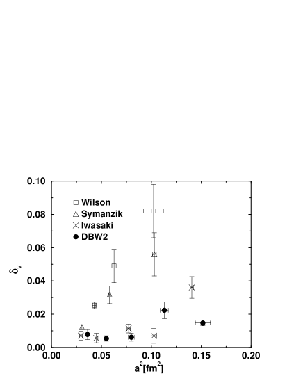
Figure 2: Rotational symmetry violation $\delta_{V}$ versus $a^{2}$ for various improved actions.

In the figure, the horizontal axis is the lattice spacing squared so as to see the expected $O(a^{2})$ violation. As seen in the figure, both Iwasaki and DBW2 actions show excellent restoration of rotational symmetry even at $a\sim 0.3$fm while clear $a^{2}$ violations are seen for plaquette and tree-level Symanzik actions.

A second check is the scaling of $T_{c}/\sqrt{\sigma}$. The critical temperature is defined as

$$T_{c}=1/N_{t}a_{c}\ ,\ \ \ a_{c}=a(\beta_{c})$$ (29)

where $N_{t}$ is the temporal lattice size. In order to obtain the critical coupling $\beta_{c}$ , $N_{t}=3,4,6$ lattices are used and the Polyakov loop susceptibility is measured. Here, histogram method is utilized to determine the peak of the susceptibility.[18] Then, $\beta_{c}$ at infinite volume limit is obtained by finite size scaling of $12^{3}\times 4$ and $16^{3}\times 4$ lattices. The resulting $\beta_{c}$ are given in Table 3.

$N_{t}$	$N_{s}$	$(\beta_{11}+8\beta_{12})_{c}\ \ \mbox{at}\ \ V=\infty$
3	10, 12, 14	0.75696(98)
4	12, 16	0.82430(95)
6	18	0.9636(25)

Table 3: Phase transition points for the DBW2 action at finite temperature. Results are obtained by extrapolating to the infinite volume limit.

The string tension is measured on $12^{3}\times 24$ and $18^{3}\times 36$ lattices at the values of the coupling determined by the $T_{c}$ analysis. It is extracted from the static quark potential using the Ansatz ;

$$V(R)=A+{\alpha\over R}+\sigma R$$ (30)

$\beta_{11}+8\beta_{12}$	$A$	$\alpha$	$\sigma a^{2}$
0.82430	0.550(17)	-0.255(23)	0.1555(28)
0.9636	0.5791(96)	-0.357(22)	0.06996(99)

Table 4: Parameters of the heavy quark potential for the DBW2 action. These simulations are carried out on $12^{3}\times 24$ and $18^{3}\times 36$ lattices while the values of the coupling are those determined by $T_{c}$ analysis (Table 3). Statistics is 130 configurations per data at $\beta_{11}+8\beta_{12}=0.82430$ and 80 configurations per data at $\beta_{11}+8\beta_{12}=0.9636$.

From the extracted values of $\sigma$ at $\beta_{c}(N_{t}=3)$, $\beta_{c}(N_{t}=4)$ and $\beta_{c}(N_{t}=6)$ we obtain the following values of $T_{c}/\sqrt{\sigma}$:

$$T_{c}/\sqrt{\sigma}= 0.6340(60)\ \ \ {\rm at}\ \ \ N_{t}=4$$ (31)

$$0.6301(65)\ \ \ {\rm at}\ \ \ N_{t}=6$$

In Fig. 3 we show the obtained results together with other data from plaquette (Wilson), tree-level Symanzik, tadpole improved Symanzik and Iwasaki actions taken from Refs [19, 20].

Figure 3: Scaling behavior of $T_{c}/\sqrt{\sigma}$. We compare the DBW2 action with results from other actions in two-coupling space [19, 20].

No appreciable dependence on the lattice spacing is seen in the ratio $T_{c}/\sqrt{\sigma}$ for all the cases including the DBW2 action.

The results of both tests is an indication that the DBW2 action is a well-improved action as suggested by the non-perturbative RG flow analysis.

As a by-product of the $T_{c}$ analysis, contours of constant lattice spacing are obtained through the relation $a=1/N_{t}T_{c}$. Fig. 4 shows a compilation of the phase transition points in the two coupling space for the plaquette, tree-level Symanzik, Iwasaki and DBW2 actions on $N_{t}=3\sim 12$ lattices.

Figure 4: Contours of constant $aT_{c}$ in the ($\beta_{11},\beta_{12}$)-plane. Symbols represent the phase transition points for each $N_{t}$ at the thermodynamic limit. Dotted lines connect the points with the same $aT_{c}(=1/N_{t})$ and they suggest contours of $aT_{c}=const.$.

5 A model analysis for the flow

Results of the RG flow in the section 3 provide basic information on relation between couplings and lattice spacing. In order to understand the driving force of the flow, we examine a toy model which incorporates a perturbative scaling term and an irrelevant coupling at small lattice spacing and an attraction originated from area law in strong coupling region.

We consider two dimensional model beta function which has a marginal coupling and an irrelevant one at small lattice spacing as

$${d\vec{\beta}\over d\ln a}={\bf A}\vec{\beta}-B(\beta_{n}){\vec{n}\over|\vec{n}|^{2}}$$ (32)

where $B(x)$ is the perturbative beta-function

$$B(x)=12b_{0}+72\frac{b_{1}}{x}+\cdots$$ (33)

with $b_{0}=33/(48\pi^{2})$ and $b_{1}=(102/121)b_{0}^{2}$. ${\bf A}$ is a constant $2\times 2$ matrix which has a zero eigenvalue with an eigenvector $\vec{w}$ and a negative eigenvalues $\lambda$ with a eigenvector $\vec{v}$ . $\vec{n}$ is constant vector orthogonal to $\vec{v}$ , i.e., $(\vec{n}\cdot\vec{v})=0$ . By this condition, resultant solution exibits correct scaling property for $(\vec{n}\cdot\vec{\beta})$.

Solution of eq. (32) is

$$\vec{\beta}=(ca^{\lambda}+d(a))\vec{v}+{\beta_{p}(a\Lambda)\over(\vec{n}\cdot\vec{w})}\vec{w}$$ (34)

where $\beta_{p}(a\Lambda)$ is the asymptotic scaling solution satisfying

$${d\beta_{p}\over d\ln a}=-B(\beta_{p})$$ (35)

and

$$d(a)={(\vec{v}\cdot\vec{w})\over(\vec{n}\cdot\vec{w})}\int^{1}_{0}d\xi\ \xi^{-\lambda-1}B(\beta_{p}(\xi a\Lambda))\quad.$$ (36)

It is noted that $(\vec{n}\cdot\vec{\beta})=\beta_{p}(a\Lambda).$

Attractive driving force in the strong coupling region comes in from the string tension. The lowest order of strong coupling calculation for $N\times M$ Wilson loops is (suppose that $NM$ is an even integer)

$$<W(N\times M)>=(\beta_{11}/18)^{NM}+(\beta_{11}/18)^{NM-2}(\beta_{12}/18)P^{NM}_{1}+$$

$$(\beta_{11}/18)^{NM-4}(\beta_{12}/18)^{2}P^{NM}_{2}+\cdot\cdot+(\beta_{12}/18)^{NM/2}P^{NM}_{NM/2}$$ (37)

where $P^{NM}_{k}$ are the tiling weights for filling the area of the loop by $(NM-2k)\ [1\times 1]$ and $k\ [1\times 2]$ tiles. Then, area law for the Wilson loop leads

$$\beta_{11}/18=\exp(-a^{2}\sigma),\ \ \ \ \beta_{12}/18=C\exp(-2a^{2}\sigma)\ \ .$$ (38)

In a differential form, we have

$${d\vec{\beta}\over da^{2}}=-\sigma\left(\begin{array}[]{cc}1&0\\ 0&2\\ \end{array}\right)\vec{\beta}.$$ (41)

Driving force in a two dimensional toy model beta function is assumed as sum of those in the weak and strong-coupling region,i.e.,

$${d\vec{\beta}\over ds}=-2s\left(\begin{array}[]{cc}1+{\zeta_{1}\over s}&0\\ 0&2+{\zeta_{2}\over s}\\ \end{array}\right)\vec{\beta}+{1\over s}[{\bf A}\vec{\beta}-B(\beta_{n}){\vec{n}\over|\vec{n}|^{2}}]\ \ ,\ \ \ \ s\equiv a\sqrt{\sigma}\ \ .$$ (44)

Here, we keep the next order in $a$ in the non-perturbative term as free parameters, $\zeta_{1}$ and $\zeta_{2}$. Parameters included are $\theta,\theta^{\prime},\lambda,\zeta_{1}$ and $\zeta_{2}$. $\vec{v}$ and $\vec{w}$ are specified as $\vec{v}=(\cos\theta^{\prime},\ \sin\theta^{\prime})$ and $\vec{w}=(\cos\theta,\ \sin\theta)$. Here the matrix ${\bf A}$ is ${\bf A}=\lambda\vec{v}\otimes\vec{w_{T}}^{t}/(\vec{v}\cdot\vec{w_{T}})$ with $\vec{w_{T}}=i\sigma_{2}\vec{w}$. $\vec{n}$ is given by $\vec{n}=(1,\cot(-\theta^{\prime}))$.

By this model, we calculate lattice spacings for different actions, RG flow trajectories and contours of constant lattice spacings. Comparisons with the present data and those reported in references [28, 29] are made. Giving initial conditions for $\beta_{11},\beta_{12}$ and $a$ on the $\beta_{12}=0$ line (plaquette action) [21, 23, 22] , those quantities are calculated and shown in Fig.s 5, and 6. Parameters are chosen so as to match the recently reported data of $a\sqrt{\sigma}$ for the Iwasaki action [28]

$$\theta=-0.156\ ,\ \ \theta^{\prime}=-0.205\ ,\ \ \lambda=-0.5\ ,\ \ \zeta_{1}=0.1\ \ \zeta_{2}=0.0\ .$$ (45)

As shown in the figures, lattice spacings in the $\beta_{11}-\beta_{12}$ plane and the RG flow trajectories are reasonably well reproduced. As for the flow, rapid approach to the attractive stream is driven by the irrelevant coupling. At intermediate lattice spacings, both the non-perturbative and asymptotic scaling terms drive the trajectories. Finally, in the strong coupling region, the non-perturbative term dominates and the parabolic behavior of the trajectories sets on. We also note that the model describes contours of constant lattice spacing fairly well as seen in Fig.6.

Through the study, an understanding for basic driving mechanism of the RG flow in $\beta_{11}-\beta{12}$ plane by scaling term and an irrelevant coupling at small lattice spacing and an attraction originated from area law in strong coupling region is suggested.

Figure 5: (a) Lattice spacing versus $\beta_{11}$. Crosses are input data from the plaquette action given by [21, 22, 23]. Filled symbols are the data of tree-level Symanzik action (squares) and DBW2 action (diamonds) [29]. The corresponding open symbols are the results predicted by eq. (44). (b) Flow trajectories calculated by eq. (44). The trajectories start at $(\beta_{11},\beta_{12})=(5.55,0.0),(5.70,0.0),(6.20,0.0)$ and $(6.80,0.0)$. Symbols on the trajectories indicate the points corresponding to the factor two blocking where the lattice spacing is $2^{n}a_{0}(n=1,2,3,\cdots)$ with initial value $a_{0}$.

Figure 6: Contours of constant lattice spacing. Filled circles show the points with $a\sqrt{\sigma}=0.4099$ , $0.2702$ and $0.1619$ as computed by eq. (44). The data for $(aT_{c})^{-1}=4$ (open squares) and 6 (open circles) obtained by the scaling analysis (Fig. 4) are also indicated.

6 Examination of renormalization effects outside of the two coupling space

In this work, the working space is limited to two coupling space $(\beta_{11},\beta_{12})$ . We have seen an evidence that the RT locates close to that plane. Since this is a highly non trivial fact, the truncation effect which comes from the limitation of the coupling space to the two-dimensional plane should be examined. There are several indirect indications that truncation effects may be important. As seen in Fig. 1, the shape of the attractor is less clear above $\beta_{11}\sim 12$ . This suggests that the distance to the RT grows in this region.

Another point is that the resulting couplings $(\beta_{11}^{\prime},\beta_{12}^{\prime})$ obtained through the truncation into two coupling space after blocking give larger lattice spacing (roughly 40-60 %) than that of the original blocked lattice. One possible reason is the choice of a minimal set of loops in the Schwinger-Dyson equation. But this effect might also be due to the truncation of the space of couplings. See ref. [16].

In order to examine renormalization effects outside to the two coupling space, we perform a limited analysis in a three coupling space, $(\beta_{11},\beta_{12},\beta_{\rm twist})$, with a twisted loop included in the action [26],

$$S_{\rm twist}= \beta_{\rm twist}\sum_{n,\mu\neq\nu\neq\tau}[1-{1\over 3}{\rm Re}\mbox{\rm Tr}(P_{\rm twist}^{\mu\nu\tau})]$$ (46)

where

$$P_{\rm twist}^{\mu\nu\tau}=U_{\mu}(n)U_{\nu}(n+\hat{\mu})U_{\tau}(n+\hat{\mu}+\hat{\nu})U_{-\nu}(n+\hat{\mu}+\hat{\nu}+\hat{\tau})U_{-\mu}(n+\hat{\mu}+\hat{\tau})U_{-\tau}(n+\hat{\tau}).$$ (47)

We will study $\beta_{\rm twist}$ in addtion to $(\beta_{11},\beta_{12})$ because in Ref.[17] more general actions were studied and it was found that the value of the twist coupling is larger that that of the chair type loop. Moreover the action with $W_{1\times 1}$, $W_{1\times 2}$ and $W_{\rm twist}$ is often used in the reteratures. [2, 30]. We perform the blocking transformation starting from points near the attractor in the $(\beta_{11},\beta_{12})$ plane, i.e. the $\beta_{\rm twist}=0$ sector. The results are shown in Fig. 7.

Figure 7: RG flow of SU(3) lattice gauge theory in three coupling space $(\beta_{11},\beta_{12},\beta_{\rm twist})$. Blocking is applied for the points near the attractive stream on the $(\beta_{11},\beta_{12})$-plane at $\beta_{\rm twist}=0$. The top figure shows the projection of the flow onto the $(\beta_{11},\beta_{\rm twist})$ -plane while the bottom figure is the projection onto the $(\beta_{11},\beta_{12})$ -plane.

As shown in the figure, no sizable value of $\beta_{\rm twist}$ is generated for points on the attractor. On the other hand, if we start from the points $\beta_{11}\sim 10,\beta_{12}\sim-1.0$ , a negative $\beta_{\rm twist}$ is induced. This indicates that the attractor in three coupling space sits below the $\beta_{{\rm twist}}=0$ sector in this region. Although more extensive studies are necessary to clarify the exact situation, it seems that the attractor in two coupling space gives a good starting point for designing improved actions.

7 Summary

We investigate the renormalization group (RG) flow of SU(3) lattice gauge theory in a two coupling space, $(\beta_{11},\beta_{12})$. An extensive numerical calculation of the RG flow on the lattice is made. Swendsen’s blocking followed by an effective action search using the Schwinger-Dyson method is adopted to find renormalization effects. In our previous analysis, we adopted the Demon method. Although both methods give similar results, the Schwinger-Dyson algorithm is more echonomical because in case of the Demon formula we need an additional Monte Carlo simulation for each configuration. Moreover the Schwinger-Dyson method uses larger loops to determine the couplings.

Analyses are performed in the fourth quadrant of the coupling space and reveal the presence of an attractive stream. Trajectories are first attracted towards this stream and afterwards they move towards the origin along it. The stream converges to a parabolic curve in the strong coupling region. These features indicate that the RT locates close to the two coupling space and the attractive stream traces the RT.

A model flow equation which consists of asymptotic scaling, an irrelevant coupling and a non-perturbative force corresponding to the area law can reproduce the observed features.

In this paper we have compared several actions in the two coupling space by measuring the restoration of the rotational symmetry and the scaling of $\sqrt{\sigma}/T_{c}$. In the regions of $a\sim 0.3$, Iwasaki and DBW2 actions, which are near to RT , are superior to tree-level Symanzik and plaquette actions. Although ”improveness” of all actions are indistinguishable at smaller lattice spacing within the present statistics, this indicate that nonperturbative study of RG flows is valuable to design an improved action at intermediate lattice spacing. It is highly desirable to pursue the same analysis for fermion actions.

The effect of truncation to a space with only two couplings is partly examined and it is found that renormalization effects outside the two coupling space are small and the attractive stream in this space gives hence a good starting point for improvement.

8 Acknowledgments

All simulations have been done on CRAY J90 at Information Processing Center, Hiroshima University, SX-4 at RCNP, Osaka University and on VPP500 at KEK (High Energy Accelerator Research Organization). The authors would like to acknowledge M. Okawa for discussions on the Schwinger-Dyson method. They acknowledge also G. Bali for performing the measurement of the heavy quark potential. H. Matsufuru would like to thank the Japan Society for the Promotion of Science for financial support. This work is supported by the Grant-in-Aide for Scientific Research by Monbusho, Japan (No. 11694085) and (No. 10640272). This work is supported also by the Supercomputer Project No32 (FY1998) of High Energy Accelerator Research Organization (KEK).

References

- [1] K. G. Wilson, in Recent Developments in Gauge theories, ed. G. t’Hooft (Plenum Press, New York, 1980) p. 363.
- [2] R. Gupta, “The Renormalization Group and lattice QCD”, From Actions to Answers, ed. T. DeGrand and D. Toussaint, World Scientific 1990; INTRODUCTION TO LATTICE QCD: COURSE Lectures given at Les Houches Summer School in Theoretical Physics, Session 68: Probing the Standard Model of Particle Interactions, Les Houches, France, 28 Jul - 5 Sep 1997.
- [3] QCD-TARO Collaboration, Phys. Rev. Lett. 71 (1993) 3063.
- [4] A. González-Arroyo and M. Okawa, Phys. Rev. D35 (1987) 672; Phys. Rev. B35 (1987) 2108.
- [5] M. Hasenbusch, K. Pinn and C. Wieczerkowski, Phys. Lett. B338 (1994) 308.
- [6] T. Takaishi, Mod. Phys. Lett. A10 (1995) 503.
- [7] A. Patel and R. Gupta, Phys. Lett. B183 (1987) 193.
- [8] Y. Iwasaki, University of Tsukuba preprint, UTHEP-118, 1983.
- [9] P. Hasenfratz, F. Niedermayer, Nucl. Phys. B414 (1994) 785
- [10] Ph. de Forcrand et al., QCD-TARO Collaboration, Nucl. Phys. B(Proc. Suppl.)53 (1997) 938.
- [11] R. H. Swendsen, Phys. Rev. Lett. 47 (1981) 1775.
- [12] M. Creutz, Phys. Rev. Lett. 50 (1983) 1411 ; M. Hasenbush, K. Pinn, and C. Wieczerkowski, Phys. Lett. B338 (1994) 308.
- [13] M. Creutz, Quarks, gluons and lattices, Cambridge Univ Press, 1985, Chapter 10.
- [14] K. Symanzik, Nucl. Phys. B226 (1983) 187.
- [15] S. Itoh, Y. Iwasaki and T. Yoshie, Phys. Rev. D33 (1986) 1806.
- [16] T. Takaishi and Ph. de Forcrand, Phys. Lett. B428 (1998) 157
- [17] T. Takaishi, Phys. Rev. D54 (1996) 1050.
- [18] I. R. McDonald and K. Singer, Discuss. Faraday, Soc. 43 (1967) 40; A. M. Ferrenberg and R. H. Swendsen, Phys. Rev. Lett. 61 (1988) 2635, 63 (1989) 1195.
- [19] Y. Iwasaki and K. Kanaya, K. Kaneko, T. Yoshié, Phys. Rev. D56 (1997) 151.
- [20] B. Beinlich, F. Karsch, E. Laermann and A. Peikert, Eur. Phys. J. C6 (1999) 133.
- [21] G. S. Bali and K. Schilling, Phys. Rev. D46 (1992) 2636.
- [22] G. Boyd, J. Engels, F. Karsch, E. Laermann, C. Legeland, M. Lütgemeier and B. Petersson, Nucl. Phys. B469 (1996) 419.
- [23] S. Aoki et al., CP-PACS collaboration, Phys. Rev. Lett. 84 (2000) 238.
- [24] F. Karsch with B. Beinlich, J. Engels, R. Joswig, E. Laermann, A. Peikert and B. Petersson, Nucl. Phys. B(Proc. Suppl.)53 (1997) 413.
- [25] Ph. de Forcrand et al., QCD-TARO collaboration, Nucl. Phys. B(Proc. Suppl.)63A-C (1998) 928.
- [26] Ph. de Forcrand et al., QCD-TARO collaboration, Nucl. Phys. B(Proc. Suppl.)73 (1999) 924.
- [27] Ph. de Forcrand et al., QCD-TARO collaboration, Proceedings of the LATTICE99, Pisa,1999, to appear in Nucl. Phys. B(Proc. Suppl.).
- [28] M. Okamoto et al., CP-PACS collaboration, Phys. Rev. D60 (1999) 094510.
- [29] A. Boriçi and R. Rosenfelder, Nucl. Phys. B(Proc. Suppl.)63A-C (1998) 925.
- [30] M. Alford, W. Dimm, G.P. Lepage, G. Hockney and P.B. Mackenzie, Nucl. Phys. B (Proc. Suppl.) 42 (1995) 787.