Nucleon Decay Matrix Elements from Lattice QCD

Abstract

We present a model-independent calculation of hadron matrix elements for all dimension-six operators associated with baryon number violating processes using lattice QCD. The calculation is performed with the Wilson quark action in the quenched approximation at $\beta=6/g^{2}=6.0$ on a $28^{2}\times 48\times 80$ lattice. Our results cover all the matrix elements required to estimate the partial lifetimes of (proton,neutron)$\rightarrow$($\pi,K,\eta$) +(${\bar{\nu}},e^{+},\mu^{+}$) decay modes. We point out the necessity of disentangling two form factors that contribute to the matrix element; previous calculations did not make the separation, which led to an underestimate of the physical matrix elements. With a correct separation, we find that the matrix elements have values $3-5$ times larger than the smallest estimates employed in phenomenological analyses of the nucleon decays, which could give strong constraints on several GUT models. We also find that the values of the matrix elements are comparable with the tree-level predictions of chiral lagrangian.

I Introduction

Nucleon decay is one of the most exciting predictions of grand unified theories (GUTs) regardless of the existence of supersymmetry (SUSY). Although none of the decay modes have been detected up to now, experimental efforts over the years have pushed the lower limit on the partial lifetimes of the nucleon. Moreover, an improvement by an order of magnitude is expected from the Super-Kamiokande experiment, which can give a strong constraint on (SUSY-)GUTs. On the other hand, theoretical predictions of the nucleon partial lifetimes suffer from various uncertainties. One of the main sources of uncertainties is found in the evaluation of the hadron matrix elements for the nucleon decays $\langle PS|{\cal O}^{{{B}{/}}}|N\rangle$, where $PS$ and $N$ denote the pseudoscalar meson and the nucleon, and ${\cal O}^{{{B}{/}}}$ is the baryon number violating operator that appears in the low-energy effective lagrangian of (SUSY-)GUTs. The matrix elements have been estimated by employing various QCD models. Their results, however, scatter over the range whose minimum and maximum values differ by a factor of ten[1]. Therefore, a precise determination of the nucleon decay matrix elements from the first principles using lattice QCD is of extreme importance.

In lattice QCD the pioneering studies for the nucleon decay matrix elements[2, 3] attempted to estimate the matrix element $\langle\pi^{0}|{\cal O}^{{{B}{/}}}|p\rangle$, which is relevant to the dominant decay mode $p\rightarrow\pi^{0}+e^{+}$ in the minimal SU(5) GUT, from the matrix element $\langle 0|{\cal O}^{{{B}{/}}}|p\rangle$ with the aid of chiral perturbation theory. This was followed by a direct measurement of $\langle\pi^{0}|{\cal O}^{{{B}{/}}}|p\rangle$ with the use of the three-point functions[4], which showed an unexpectedly large discrepancy between these two methods: the direct method yielded a value of the matrix element two or three times smaller than the value obtained by the indirect method. Recently we have revisited this old problem and confirmed[5] the peculiar feature when one follows the methods employed in the earlier work[4].

In this paper we report results of our effort to advance the lattice QCD calculation of the nucleon decay matrix elements in several directions. We point out that there are two form factors that contribute to the matrix element $\langle\pi^{0}|{\cal O}^{{{B}{/}}}|p\rangle$ for general lepton momentum. While only one of the form factors is relevant for the physical amplitudes as the other form factor contribution is annulled by the negligibly small lepton mass, the two contributions have to be disentangled in the lattice QCD calculation. This explains the discrepancy between the direct and indirect estimations of the proton decay matrix element found in the previous studies[4, 5] where the separation was not made.

Another important feature of our calculation is model independence. All dimension-six operators associated with baryon number violating processes are classified into four types under the requirement of SU(3)$\times$SU(2)$\times$U(1) invariance at low-energy scales[6, 7]. If one specifies the decay processes of interest, namely the processes among (proton,neutron)$\rightarrow$($\pi,K,\eta$) +(${\bar{\nu}},e^{+},\mu^{+}$), we can list a complete set of independent matrix elements in QCD, and we calculate all the matrix elements.

Other advances, which are more technical but essential for precise calculation, are the following two points: (i) flavor SU(3) breaking effect in the process with the $K$ meson in the final state is correctly taken into account by setting the strange quark mass non-degenerate with the up and down quark mass, (ii) two spatial momenta are injected to investigate the $q^{2}$ dependence of the matrix elements, where $q$ is the four-momentum transfer between the nucleon and the pseudoscalar meson.

This paper is organized as follows. In Sec. II we formulate our calculational method of the nucleon decay matrix elements. The complete set of the independent matrix elements is also presented. In Sec. III we briefly review the chiral lagrangian for the baryon number violating interactions and enumerate its tree-level predictions. Section IV contains the simulation parameters and technical details. Results for the matrix element $\langle 0|{\cal O}^{{{B}{/}}}|p\rangle$ are given in Sec. V. In Sec. VI we present the results for the nucleon decay matrix elements obtained by the direct method and compare them with the tree-level predictions of the chiral lagrangian. We also discuss the soft pion limit of the matrix elements. Our conclusions are summarized in Sec. VII.

II Formulation of the method

A Independent matrix elements for nucleon decays

One of the most important features in the study of the baryon number violating processes is that the low energy effective theory is described in terms of SU(3)$\times$SU(2)$\times$U(1) gauge symmetry based on the strong and the electroweak interactions, which enables us to make a model independent analysis. Our interest is focused on the dimension-six operators which are the lowest dimensional operators in the low energy effective Hamiltonian: operators associated with the baryon number violating processes must contain at least three quark fields to form SU(3) color singlet, and then an additional lepton field is required to construct a Lorentz scalar. Higher-dimensional operators are suppressed by inverse powers of heavy particle mass that is characterized by the theory beyond the standard model.

All dimension-six operators are classified into the four types under the requirement of SU(3)$\times$SU(2)$\times$U(1) invariance [6, 7]:

$${\cal O}^{(1)}_{abcd} = ({\bar{D}}^{c}_{iaR}U_{jbR})({\bar{Q}}^{c}_{\alpha kcL}L_{\beta dL})\epsilon_{ijk}\epsilon_{\alpha\beta},$$ (1)

$${\cal O}^{(2)}_{abcd} = ({\bar{Q}}^{c}_{\alpha iaL}Q_{\beta jbL})({\bar{U}}^{c}_{kcR}L_{dR})\epsilon_{ijk}\epsilon_{\alpha\beta},$$ (2)

$${\cal O}^{(3)}_{abcd} = ({\bar{Q}}^{c}_{\alpha iaL}Q_{\beta jbL})({\bar{Q}}^{c}_{\gamma kcL}L_{\delta dL})\epsilon_{ijk}\epsilon_{\alpha\delta}\epsilon_{\beta\gamma},$$ (3)

$${\cal O}^{(4)}_{abcd} = ({\bar{D}}^{c}_{iaR}U_{jbR})({\bar{U}}^{c}_{kcR}L_{dR})\epsilon_{ijk},$$ (4)

where ${\bar{\psi}}^{c}=\psi^{T}C$ with $C=\gamma_{4}\gamma_{2}$ the charge conjugation matrix; $i$, $j$ and $k$ are SU(3) color indices; $\alpha$, $\beta$, $\gamma$ and $\delta$ are SU(2) indices; $a$, $b$, $c$ and $d$ are generation indices; $L_{L}$ and $Q_{L}$ are generic lepton and quark SU(2) doublets with the left-handed projection $P_{L}=(1-\gamma_{5})/2$; $L_{R}$, $U_{R}$, and $D_{R}$ are generic charged lepton and quark SU(2) singlets with the right-handed projection $P_{R}=(1+\gamma_{5})/2$. Fierz transformations are used to eliminate all vector and tensor Dirac structures in eqs. (1)$-$(4).

The operators relevant to non-strange final states are[8]

$${\cal O}^{(1)}_{d} = ({\bar{d}}^{c}_{iR}u_{jR})({\bar{u}}^{c}_{kL}e_{dL}-{\bar{d}}^{c}_{kL}\nu_{dL})\epsilon_{ijk},$$ (5)

$${\cal O}^{(2)}_{d} = ({\bar{d}}^{c}_{iL}u_{jL})({\bar{u}}^{c}_{kR}e_{dR})\epsilon_{ijk},$$ (6)

$${\cal O}^{(3)}_{d} = ({\bar{d}}^{c}_{iL}u_{jL})({\bar{u}}^{c}_{kL}e_{dL}-{\bar{d}}^{c}_{kL}\nu_{dL})\epsilon_{ijk},$$ (7)

$${\cal O}^{(4)}_{d} = ({\bar{d}}^{c}_{iR}u_{jR})({\bar{u}}^{c}_{kR}e_{dR})\epsilon_{ijk}.$$ (8)

We can also list the operators relevant to strange final states[8]:

$${\tilde{\cal O}}^{(1)}_{d} = ({\bar{s}}^{c}_{iR}u_{jR})({\bar{u}}^{c}_{kL}e_{dL}-{\bar{d}}^{c}_{kL}\nu_{dL})\epsilon_{ijk},$$ (9)

$${\tilde{\cal O}}^{(2)}_{d} = ({\bar{s}}^{c}_{iL}u_{jL})({\bar{u}}^{c}_{kR}e_{dR})\epsilon_{ijk},$$ (10)

$${\tilde{\cal O}}^{(3)}_{d} = ({\bar{s}}^{c}_{iL}u_{jL})({\bar{u}}^{c}_{kL}e_{dL}-{\bar{d}}^{c}_{kL}\nu_{dL})\epsilon_{ijk},$$ (11)

$${\tilde{\cal O}}^{(4)}_{d} = ({\bar{s}}^{c}_{iR}u_{jR})({\bar{u}}^{c}_{kR}e_{dR})\epsilon_{ijk},$$ (12)

$${\tilde{\cal O}}^{(5)}_{d} = ({\bar{d}}^{c}_{iR}u_{jR})({\bar{s}}^{c}_{kL}\nu_{dL})\epsilon_{ijk},$$ (13)

$${\tilde{\cal O}}^{(6)}_{d} = ({\bar{d}}^{c}_{iL}u_{jL})({\bar{s}}^{c}_{kL}\nu_{dL})\epsilon_{ijk},$$ (14)

where $d$ denote the generation; $e_{1}=e$, $e_{2}=\mu$, $\nu_{1}=\nu_{e}$ and $\nu_{2}=\nu_{\mu}$.

We are interested in the decay processes from the nucleon to one pseudoscalar meson: (proton,neutron)$\rightarrow$($\pi,K,\eta$) +(${\bar{\nu}},e^{+},\mu^{+}$). For these decay modes we can list the complete set of independent matrix elements in QCD employing the operators of eqs. (5)$-$(14):

$$\langle\pi^{0}|\epsilon_{ijk}({u^{i}}^{T}CP_{R,L}d^{j})P_{L}u^{k}|p\rangle,$$ (15)

$$\langle\pi^{+}|\epsilon_{ijk}({u^{i}}^{T}CP_{R,L}d^{j})P_{L}d^{k}|p\rangle,$$ (16)

$$\langle K^{0}|\epsilon_{ijk}({u^{i}}^{T}CP_{R,L}s^{j})P_{L}u^{k}|p\rangle,$$ (17)

$$\langle K^{+}|\epsilon_{ijk}({u^{i}}^{T}CP_{R,L}s^{j})P_{L}d^{k}|p\rangle,$$ (18)

$$\langle K^{+}|\epsilon_{ijk}({u^{i}}^{T}CP_{R,L}d^{j})P_{L}s^{k}|p\rangle,$$ (19)

$$\langle K^{0}|\epsilon_{ijk}({u^{i}}^{T}CP_{R,L}s^{j})P_{L}d^{k}|n\rangle,$$ (20)

$$\langle\eta|\epsilon_{ijk}({u^{i}}^{T}CP_{R,L}d^{j})P_{L}u^{k}|p\rangle,$$ (21)

where we assume SU(2) isospin symmetry $m_{u}=m_{d}$ and use the relations

$$\langle PS|{\cal O}_{LR}|N\rangle = \langle PS|{\cal O}_{RL}|N\rangle,$$ (22)

$$\langle PS|{\cal O}_{RR}|N\rangle = \langle PS|{\cal O}_{LL}|N\rangle,$$ (23)

due to the parity invariance. All we have to calculate in lattice QCD are these 14 matrix elements. Other matrix elements are obtained through the exchange of the up and down quarks, under which the nucleon and PS meson states transform as

$$|p\rangle\rightarrow-|n\rangle,\;|n\rangle\rightarrow-|p\rangle,$$ (24)

$$\langle\pi^{+}|\rightarrow\langle\pi^{-}|,\;\langle\pi^{0}|\rightarrow-\langle\pi^{0}|,\;\langle\pi^{-}|\rightarrow\langle\pi^{+}|,$$ (25)

$$\langle K^{+}|\rightarrow\langle K^{0}|,\;\langle K^{0}|\rightarrow\langle K^{+}|,$$ (26)

$$\langle\eta|\rightarrow\langle\eta|,$$ (27)

where there is no decay mode with the ${\bar{K}}^{0}$ or $K^{-}$ final state.

B Form factors in nucleon decay matrix elements

Under the requirement of Lorentz and parity invariance, the matrix elements between the nucleon($N$) and the pseudoscalar(PS) meson in eqs. (15)$-$(21) can have two form factors:

$$\langle PS(\vec{p})|{\cal O}_{L}^{{{B}{/}}}|N^{(s)}(\vec{k})\rangle=P_{L}\left(W_{0}(q^{2})-W_{q}(q^{2})i{{{q}{/}}}\right)u^{(s)},$$ (28)

where ${\cal O}^{{{B}{/}}}_{L}$ represents the three-quark operator projected to the left-handed chiral state, $u^{(s)}$ denotes the Dirac spinor for nucleon with either the up ($s=1$) or down ($s=2$) spin state , and $q^{2}$ is the momentum squared of the out-going antilepton. The contribution of the $W_{q}$ term in eq.(28) is negligible in the physical decay amplitude, because its contribution is of the order of the lepton mass $m_{l}$ after the multiplication with antilepton spinor. However, since the relative magnitude of the two form factors $W_{0}$ and $W_{q}$ is a priori not known, we have to disentangle these two form factors in the lattice QCD calculation. Hereafter we refer to $W_{0}$ and $W_{q}$ as relevant and irrelevant form factor respectively.

In the lattice calculation, $\vec{k}=\vec{0}$ is chosen for the nucleon spatial momentum and $\vec{p}=\vec{k}-\vec{q}\neq\vec{0}$ for the PS meson. In this case the Dirac structure of the right hand side in eq. (28) is given by

$$\left(W_{0}-W_{q}i{{{q}{/}}}\right)u^{(s)} = \left(\begin{array}[]{cc}W_{0}-iq_{4}W_{q}&-W_{q}{\vec{q}}\cdot\vec{\sigma}\\ W_{q}{\vec{q}}\cdot\vec{\sigma}&W_{0}+iq_{4}W_{q}\end{array}\right)u^{(s)}$$ (31)

$$= \left(\begin{array}[]{cc}W_{0}+(m_{N}-\sqrt{m_{PS}^{2}+{\vec{p}}^{2}})W_{q}&W_{q}{\vec{p}}\cdot\vec{\sigma}\\ -W_{q}{\vec{p}}\cdot\vec{\sigma}&W_{0}-(m_{N}-\sqrt{m_{PS}^{2}+{\vec{p}}^{2}})W_{q}\end{array}\right)u^{(s)},$$ (34)

where $W_{0}-W_{q}i{{{q}{/}}}$ is expressed by a $2\times 2$ block notation; $\vec{\sigma}$ are the Pauli matrices, and ${u^{(s)}}^{T}=(1,0,0,0)$ or $(0,1,0,0)$. It is important to observe that the upper components of $(W_{0}-W_{q}i{{{q}{/}}})u^{(s)}$ are linear combinations of the relevant and irrelevant form factors, while the lower components contain only the irrelevant one. Therefore, we can extract the relevant form factor $W_{0}$ from the upper components by subtracting the contribution of the irrelevant form factor $W_{q}$ with the use of the lower components.

The need for the separation of the contribution of the irrelevant form factor was not recognized in the previous studies with the direct method[4, 5]. The values found in these studies correspond to $W_{0}-iq_{4}W_{q}$ instead of $W_{0}$. We examine how much this affects the estimate of the matrix elements in Sec. VI.

Let us add several technical comments: (i) The separation procedure described above cannot be applied to the case of ${\vec{p}}={\vec{k}}={\vec{0}}$ because of vanishing lower components. (ii) Another possible choice of momenta for disentangling the relevant and irrelevant form factors is given by ${\vec{k}}\neq{\vec{0}}$ and ${\vec{p}}={\vec{0}}$. In this case, however, we cannot achieve $-q^{2}=m_{l}^{2}$.

C Calculational methods

The nucleon decay matrix elements of eq. (28) are calculated with two methods, which we refer to as the direct and the indirect method. The former is to extract the matrix elements from the three-point function of the nucleon, the PS meson and the baryon number violating operator. The latter is to estimate them with the aid of chiral lagrangian, where we have two unknown parameters to be determined by the lattice QCD calculation.

In the direct method we calculate the following ratio of the hadron three-point function divided by the two-point functions:

$$R(t,t^{\prime}) = \frac{\sum_{{\vec{x}},{\vec{x}}^{\prime}}{\rm e}^{i{\vec{p}}\cdot({\vec{x}}^{\prime}-{\vec{x}})}\langle{J}_{PS}({\vec{x}}^{\prime},t^{\prime}){\hat{\cal O}}^{{{B}{/}}}_{L,\gamma}({\vec{x}},t)\bar{J^{\prime}}_{N,s}(0)\rangle}{\sum_{{\vec{x}},{\vec{x}}^{\prime}}{\rm e}^{i{\vec{p}}\cdot({\vec{x}}^{\prime}-{\vec{x}})}\langle{J}_{PS}({\vec{x}}^{\prime},t^{\prime}){J}_{PS}^{\dagger}({\vec{x}},t)\rangle\sum_{\vec{x}}\langle{J}_{N,s}({\vec{x}},t)\bar{J}^{\prime}_{N,s}(0)\rangle}\sqrt{Z_{PS}}\sqrt{Z_{N}}$$ (35)

$$\longrightarrow \frac{1}{L_{x}L_{y}L_{z}}\langle PS(\vec{p})|{\hat{\cal O}}^{{{B}{/}}}_{L,\gamma}|N^{(s)}({\vec{k}}={\vec{0}})\rangle\;\;\;\;\;\;\;\;t^{\prime}\gg t\gg 0.$$ (36)

Here ${\hat{\cal O}}^{{{B}{/}}}_{L,\gamma}$ denotes the renormalized operator in the naive dimensional regularization(NDR) with the ${\overline{\rm MS}}$ subtraction scheme, and $\gamma$ and $s$ are spinor indices; we can specify the spin state of the initial nucleon at rest by choosing $s=1$ or $2$. $L_{x}L_{y}L_{z}$ is the spatial volume of lattice in lattice units. The amplitudes $Z_{PS}$ and $Z_{N}$ are given by

$$\langle PS(\vec{p})|{J}_{PS}^{\dagger}({\vec{0}},0)|0\rangle = \sqrt{Z_{PS}},$$ (37)

$$\langle 0|{J}_{N,s}({\vec{0}},0)|N^{(s^{\prime})}({\vec{0}})\rangle = \sqrt{Z_{N}}u_{s}^{(s^{\prime})},$$ (38)

which can be obtained from the two-point functions

$$\sum_{{\vec{x}},{\vec{x}}^{\prime}}{\rm e}^{i{\vec{p}}\cdot({\vec{x}}^{\prime}-{\vec{x}})}\langle{J}_{PS}({\vec{x}}^{\prime},t^{\prime}){J}_{PS}^{\dagger}({\vec{x}},t)\rangle,$$ (39)

$$\sum_{\vec{x}}\langle{J}_{N,s}({\vec{x}},t)\bar{J}_{N,s}({\vec{0}},0)\rangle.$$ (40)

We move the baryon number violating operator ${\hat{\cal O}}^{{{B}{/}}}_{L,\gamma}$ in terms of $t$ between the nucleon source placed at $t=0$ and the PS meson sink fixed at some $t^{\prime}$ well separated from $t=0$.

We list all the local interpolating fields for the PS meson and the nucleon required to calculate the independent matrix elements of eqs. (15)$-$(21):

$${J}_{\pi^{0}}({\vec{x}},t) = \frac{1}{\sqrt{2}}\left({\bar{u}}(\vec{x},t)\gamma_{5}u(\vec{x},t)-{\bar{d}}(\vec{x},t)\gamma_{5}d(\vec{x},t)\right),$$ (41)

$${J}_{\pi^{+}}({\vec{x}},t) = {\bar{d}}(\vec{x},t)\gamma_{5}u(\vec{x},t),$$ (42)

$${J}_{K^{0}}({\vec{x}},t) = {\bar{s}}(\vec{x},t)\gamma_{5}d(\vec{x},t),$$ (43)

$${J}_{K^{+}}({\vec{x}},t) = {\bar{s}}(\vec{x},t)\gamma_{5}u(\vec{x},t),$$ (44)

$${J}_{\eta}({\vec{x}},t) = \frac{1}{\sqrt{6}}\left({\bar{u}}(\vec{x},t)\gamma_{5}u(\vec{x},t)+{\bar{d}}(\vec{x},t)\gamma_{5}d(\vec{x},t)-2{\bar{s}}(\vec{x},t)\gamma_{5}s(\vec{x},t)\right),$$ (45)

$${J}_{p,s}({\vec{x}},t) = \epsilon_{ijk}\left({u^{i}}^{T}(\vec{x},t)C\gamma_{5}d^{j}(\vec{x},t)\right)u^{k}_{s}(\vec{x},t),$$ (46)

$${J}_{n,s}({\vec{x}},t) = \epsilon_{ijk}\left({u^{i}}^{T}(\vec{x},t)C\gamma_{5}d^{j}(\vec{x},t)\right)d^{k}_{s}(\vec{x},t).$$ (47)

We also prepare smeared operators for the nucleon source to overlap with the lowest energy state dominantly:

$${J}^{\prime}_{p,s}(t) = \sum_{{\vec{x}},{\vec{y}},{\vec{z}}}\Psi({\vec{x}})\Psi({\vec{y}})\Psi({\vec{z}})\epsilon_{ijk}\left({u^{i}}^{T}(\vec{x},t)C\gamma_{5}d^{j}(\vec{y},t)\right)u^{k}_{s}(\vec{z},t),$$ (48)

$${J}^{\prime}_{n,s}(t) = \sum_{{\vec{x}},{\vec{y}},{\vec{z}}}\Psi({\vec{x}})\Psi({\vec{y}})\Psi({\vec{z}})\epsilon_{ijk}\left({u^{i}}^{T}(\vec{x},t)C\gamma_{5}d^{j}(\vec{y},t)\right)d^{k}_{s}(\vec{z},t),$$ (49)

where the measured quark wave function in the pion is employed for the smearing factor $\Psi$, which is obtained by

$$\frac{\sum_{\vec{y}}\langle{\bar{d}}(\vec{x},t)\gamma_{5}u(\vec{0},t){\bar{u}}(\vec{y},0)\gamma_{5}d(\vec{y},0)\rangle}{\sum_{\vec{y}}\langle{\bar{d}}(\vec{0},t)\gamma_{5}u(\vec{0},t){\bar{u}}(\vec{y},0)\gamma_{5}d(\vec{y},0)\rangle}\longrightarrow\Psi({\vec{x}})\;\;\;\;\;\;\;\;t\gg 0$$ (50)

with configurations fixed to the Coulomb gauge. Although there is no reason to assume that the wave functions for the three quarks in the proton is well described by the quark wave function in the pion, the smeared sources of eqs. (48) and (49) work effectively (see Sec. V).

In the renormalization of the baryon number violating operators on the lattice, the explicit chiral symmetry breaking in the Wilson quark action causes mixing between operators with different chiralities. In eqs. (15)$-$(21) we find two types of operators in terms of chiralities:

$${\cal O}_{RL}=\epsilon_{ijk}{(\psi^{i}_{1}}^{T}CP_{R}\psi^{j}_{2})P_{L}\psi^{k}_{3},$$ (51)

$${\cal O}_{LL}=\epsilon_{ijk}{(\psi^{i}_{1}}^{T}CP_{L}\psi^{j}_{2})P_{L}\psi^{k}_{3},$$ (52)

where $\psi_{1,2,3}$ represent the quark fields. Their mixing structures under perturbative renormalization up to one-loop level are given by[9]

$${\cal O}_{RL}^{\rm cont}(\mu) = Z(\alpha_{s},\mu a){\cal O}_{RL}^{\rm latt}(a)+\frac{\alpha_{s}}{4\pi}Z_{mix}{\cal O}_{LL}^{\rm latt}(a)-\frac{\alpha_{s}}{4\pi}Z_{mix}^{\prime}{\cal O}_{\gamma_{\mu}L}^{\rm latt}(a),$$ (53)

$${\cal O}_{LL}^{\rm cont}(\mu) = Z(\alpha_{s},\mu a){\cal O}_{LL}^{\rm latt}(a)+\frac{\alpha_{s}}{4\pi}Z_{mix}{\cal O}_{RL}^{\rm latt}(a)+\frac{\alpha_{s}}{4\pi}Z_{mix}^{\prime}{\cal O}_{\gamma_{\mu}L}^{\rm latt}(a),$$ (54)

where the overall factor $Z(\alpha_{s},\mu a)$ has the form

$$Z(\alpha_{s},\mu a)=1+\frac{\alpha_{s}}{4\pi}\left(4{\rm ln}(\mu a)+\Delta_{{{B}{/}}}\right),\\$$ (55)

with $\mu$ the renormalization scale, and the additional operator ${\cal O}_{\gamma_{\mu}L}$ is defined by

$${\cal O}_{\gamma_{\mu}L}=\epsilon_{ijk}{(\psi^{i}_{1}}^{T}C\gamma_{\mu}\gamma_{5}\psi^{j}_{2})P_{L}\gamma_{\mu}\psi^{k}_{3}.$$ (56)

Employing the $\overline{\rm MS}$ subtraction scheme with the naive dimensional regularization for the continuum theory, we have reevaluated the finite constants and found

$$\Delta_{{{B}{/}}} = -34.11\hskip 24.0pt{\rm for\hskip 12.0ptNDR},$$ (57)

$$Z_{mix} = 3.21,$$ (58)

$$Z_{mix}^{\prime} = -0.803,$$ (59)

where the errors are $\pm 1$ in the last digit. The value of $\Delta_{{{B}{/}}}$ depends on the renormalization scheme in the continuum, while $Z_{mix}$ and $Z^{\prime}_{mix}$ are independent. We present the integral for $\Delta_{{{B}{/}}}$ in the dimensional reduction(DRED) scheme and those for $Z_{mix}$ and $Z^{\prime}_{mix}$ in Appendix, where we give a detailed description for the one-loop perturbative calculation of the renormalization factors. With the use of the KLM normalization of quark fields[10] and the tadpole improvement[11], the overall renormalization factor of eq. (55) is rewritten as

$$Z(\alpha_{s},\mu a)=\left(1-\frac{3K}{4K_{c}}\right)^{\frac{3}{2}}\left[1+\frac{\alpha_{s}}{4\pi}\left(4{\rm ln}(\mu a)+\Delta_{{{B}{/}}}+\frac{3}{2}\pi\times 5.457\right)\right].$$ (60)

Here $K_{c}$ is the critical hopping parameter at which the pion mass vanishes. We use

$$\frac{1}{8K_{c}}=1-5.457\alpha_{s}/4$$ (61)

in Ref. [12] for the perturbative estimate of $K_{c}$.

Let us turn to the indirect method. The baryon number violating operators constructed in chiral lagrangian contains two unknown coefficients $\alpha$ and $\beta$ defined by

$$\langle 0|\epsilon_{ijk}({u^{i}}^{T}CP_{R}d^{j})P_{L}u^{k}|p^{(s)}\rangle = \alpha P_{L}u^{(s)},$$ (62)

$$\langle 0|\epsilon_{ijk}({u^{i}}^{T}CP_{L}d^{j})P_{L}u^{k}|p^{(s)}\rangle = \beta P_{L}u^{(s)},$$ (63)

where operators are renormalized in the NDR scheme with the use of the renormalization factors of eqs. (58)$-$ (60). These matrix elements are obtained from the two-point functions:

$$R^{\alpha\beta}(t) = \frac{\sum_{\vec{x}}\langle\epsilon_{ijk}({u^{i}}^{T}CP_{R,L}d^{j})P_{L}u^{k}({\vec{x}},t)\bar{J}^{\prime}_{p,s}(0)\rangle}{\sum_{\vec{x}}\langle{J}_{p,s}({\vec{x}},t)\bar{J}^{\prime}_{p,s}(0)\rangle}\sqrt{Z_{N}}$$ (64)

$$\longrightarrow \langle 0|\epsilon_{ijk}(u^{i}CP_{R,L}d^{j})P_{L}u^{k}|p^{(s)}\rangle\;\;\;\;\;\;\;\;t\gg 0.$$ (65)

Incorporating the $\alpha$ and $\beta$ values determined by the lattice calculation in the tree-level results of chiral lagrangian, we can evaluates the nucleon decay matrix elements of eqs. (15)$-$(21).

III Tree-level results of chiral lagrangian

For some nucleon decay matrix elements, tree-level results of chiral lagrangian have already been given in Refs. [8, 13], which are obtained with the use of the on-shell condition of the out-going leptons: $-q^{2}=m_{l}^{2}$ and $i{{q}{/}}v_{l}=m_{l}v_{l}$. In our lattice calculations, however, the lepton momentum is generally off the mass shell. Hence we need to understand the $q$ dependence for an extrapolation of the matrix elements to the physical point. In this section we present the tree-level results for all the independent matrix elements in eqs. (15)$-$(21) with the explicit expressions of $q$ dependences.

We first define the chiral lagrangian for baryon-meson strong interactions following the notation of Ref. [8]. The PS meson and baryon fields are given by

$$\phi = \left(\begin{array}[]{ccc}\frac{1}{\sqrt{2}}\pi^{0}+\frac{1}{\sqrt{6}}\eta&\pi^{+}&K^{+}\\ \pi^{-}&-\frac{1}{\sqrt{2}}\pi^{0}+\frac{1}{\sqrt{6}}\eta&K^{0}\\ K^{-}&{\bar{K}}^{0}&-\frac{2}{\sqrt{6}}\eta\\ \end{array}\right),$$ (69)

$$B = \left(\begin{array}[]{ccc}\frac{1}{\sqrt{2}}\Sigma^{0}+\frac{1}{\sqrt{6}}\Lambda^{0}&\Sigma^{+}&p\\ \Sigma^{-}&-\frac{1}{\sqrt{2}}\Sigma^{0}+\frac{1}{\sqrt{6}}\Lambda^{0}&n\\ \Xi^{-}&\Xi^{0}&-\frac{2}{\sqrt{6}}\Lambda^{0}\\ \end{array}\right).$$ (73)

In terms of $\phi$ we define the $3\times 3$ special unitary matrices:

$$\Sigma={\rm exp}\left(\frac{2i\phi}{f}\right),$$ (74)

$$\xi={\rm exp}\left(\frac{i\phi}{f}\right),$$ (75)

where $f$ is the pion decay constant. Under SU(3)${}_{L}\times$SU(3)_R the meson and baryon fields transform as

$$\Sigma\rightarrow L\Sigma R^{\dagger},$$ (76)

$$B\rightarrow UBU^{\dagger},$$ (77)

where $L$ is an element of SU(3)_L and $R$ is an element of SU(3)_R; $U$ is defined through the transformation properties of $\xi$:

$$\xi\rightarrow L\xi U^{\dagger}=U\xi R^{\dagger}.$$ (78)

The lowest order of the SU(3)${}_{L}\times$SU(3)_R invariant chiral lagrangian is given by

$${\cal L}_{0} = \frac{f^{2}}{8}{\rm Tr}(\partial_{\mu}\Sigma)(\partial_{\mu}\Sigma^{\dagger})+{\rm Tr}{\bar{B}}(\gamma_{\mu}\partial_{\mu}+M_{B})B$$ (82)

$$+\frac{1}{2}{\rm Tr}{\bar{B}}\gamma_{\mu}[\xi\partial_{\mu}\xi^{\dagger}+\xi^{\dagger}\partial_{\mu}\xi]B+\frac{1}{2}{\rm Tr}{\bar{B}}\gamma_{\mu}B[(\partial_{\mu}\xi)\xi^{\dagger}+(\partial_{\mu}\xi^{\dagger})\xi]$$

$$-\frac{1}{2}(D-F){\rm Tr}{\bar{B}}\gamma_{\mu}\gamma_{5}B[(\partial_{\mu}\xi)\xi^{\dagger}-(\partial_{\mu}\xi^{\dagger})\xi]$$

$$+\frac{1}{2}(D+F){\rm Tr}{\bar{B}}\gamma_{\mu}\gamma_{5}[\xi\partial_{\mu}\xi^{\dagger}-\xi^{\dagger}\partial_{\mu}\xi]B$$

on the Euclidean space-time. Quark mass contributions can be included by adding the symmetry-breaking term

$${\cal L}_{1} = -v^{3}{\rm Tr}(\Sigma^{\dagger}M_{q}+M_{q}\Sigma)$$ (85)

$$-a_{1}{\rm Tr}{\bar{B}}(\xi^{\dagger}M_{q}\xi^{\dagger}+\xi M_{q}\xi)B-a_{2}{\rm Tr}{\bar{B}}B(\xi^{\dagger}M_{q}\xi^{\dagger}+\xi M_{q}\xi)$$

$$-b_{1}{\rm Tr}{\bar{B}}\gamma_{5}(\xi^{\dagger}M_{q}\xi^{\dagger}-\xi M_{q}\xi)B-b_{2}{\rm Tr}{\bar{B}}\gamma_{5}B(\xi^{\dagger}M_{q}\xi^{\dagger},-\xi M_{q}\xi),$$

where

$$M_{q}=\left(\begin{array}[]{ccc}m_{u}&0&0\\ 0&m_{d}&0\\ 0&0&m_{s}\\ \end{array}\right).$$ (86)

The parameter $v$ is related to the meson mass by

$$v=\frac{f^{2}m_{\pi^{\pm,0}}^{2}}{4(m_{u}+m_{d})}=\frac{f^{2}m_{K^{\pm}}^{2}}{4(m_{u}+m_{s})}=\frac{f^{2}m_{K^{0}}^{2}}{4(m_{d}+m_{s})}=\frac{3f^{2}m_{\eta}^{2}}{4(m_{u}+m_{d}+4m_{s})}.$$ (87)

Experimental results for the semileptonic baryon decays give $F=0.47$ and $D=0.80$[14]. The symmetry-breaking parameters $a_{1}$ and $a_{2}$ are estimated from mass splittings among the octet baryons; $b_{1}$ and $b_{2}$, on the other hand, are not well determined since they do not contribute to the baryon masses. The parameters $v$, $a_{1}$ and $a_{2}$ have no contribution to the tree-level results for the nucleon decay matrix elements.

Let us consider the construction of the operators of eqs. (5)$-$(14), which are written in the quark fields, with the meson and baryon fields. The operators transform under SU(3)${}_{L}\times$SU(3)_R as

$$(3,{\bar{3}}) : {\cal O}_{d}^{(1)},{\tilde{\cal O}}_{d}^{(1)},{\tilde{\cal O}}_{d}^{(5)},$$ (88)

$$({\bar{3}},3) : {\cal O}_{d}^{(2)},{\tilde{\cal O}}_{d}^{(2)},$$ (89)

$$(8,1) : {\cal O}_{d}^{(3)},{\tilde{\cal O}}_{d}^{(3)},{\tilde{\cal O}}_{d}^{(6)},$$ (90)

$$(1,8) : {\cal O}_{d}^{(4)},{\tilde{\cal O}}_{d}^{(4)}.$$ (91)

These transformation properties are realized by $\xi B\xi\in(3,{\bar{3}})$, $\xi^{\dagger}B\xi^{\dagger}\in({\bar{3}},3)$ $\xi B\xi^{\dagger}\in(8,1)$ and $\xi^{\dagger}B\xi\in(1,8)$, with which we can express the operators of eqs. (5)$-$(14) as

$${\cal O}^{(1)}_{d} = \alpha\left({\bar{e}}^{c}_{dL}{\rm Tr}{\cal F}\xi B_{L}\xi-{\bar{\nu}}^{c}_{dL}{\rm Tr}{\cal F}^{\prime}\xi B_{L}\xi\right),$$ (92)

$${\cal O}^{(2)}_{d} = \alpha{\bar{e}}^{c}_{dR}{\rm Tr}{\cal F}\xi^{\dagger}B_{R}\xi^{\dagger},$$ (93)

$${\cal O}^{(3)}_{d} = \beta\left({\bar{e}}^{c}_{dL}{\rm Tr}{\cal F}\xi B_{L}\xi^{\dagger}-{\bar{\nu}}^{c}_{dL}{\rm Tr}{\cal F}^{\prime}\xi B_{L}\xi^{\dagger}\right),$$ (94)

$${\cal O}^{(4)}_{d} = \beta{\bar{e}}^{c}_{dR}{\rm Tr}{\cal F}\xi^{\dagger}B_{R}\xi,$$ (95)

$${\tilde{\cal O}}^{(1)}_{d} = \alpha\left({\bar{e}}^{c}_{dL}{\rm Tr}{\tilde{\cal F}}\xi B_{L}\xi-{\bar{\nu}}^{c}_{dL}{\rm Tr}{\tilde{\cal F}}^{\prime}\xi B_{L}\xi\right),$$ (96)

$${\tilde{\cal O}}^{(2)}_{d} = \alpha{\bar{e}}^{c}_{dR}{\rm Tr}{\tilde{\cal F}}\xi^{\dagger}B_{R}\xi^{\dagger},$$ (97)

$${\tilde{\cal O}}^{(3)}_{d} = \beta\left({\bar{e}}^{c}_{dL}{\rm Tr}{\tilde{\cal F}}\xi B_{L}\xi^{\dagger}-{\bar{\nu}}^{c}_{dL}{\rm Tr}{\tilde{\cal F}}^{\prime}\xi B_{L}\xi^{\dagger}\right),$$ (98)

$${\tilde{\cal O}}^{(4)}_{d} = \beta{\bar{e}}^{c}_{dR}{\rm Tr}{\tilde{\cal F}}\xi^{\dagger}B_{R}\xi,$$ (99)

$${\tilde{\cal O}}^{(5)}_{d} = \alpha{\bar{\nu}}^{c}_{dL}{\rm Tr}{\tilde{\cal F}}^{\prime\prime}\xi B_{L}\xi,$$ (100)

$${\tilde{\cal O}}^{(6)}_{d} = \beta{\bar{\nu}}^{c}_{dL}{\rm Tr}{\tilde{\cal F}}^{\prime\prime}\xi B_{L}\xi^{\dagger},$$ (101)

where $\alpha$ and $\beta$, which are already defined in eqs. (62) and (63), are unknown coefficients associated with the $(3,{\bar{3}})$ and $({\bar{3}},3)$ operators and the $(8,1)$ and $(1,8)$ operators respectively; ${\cal F}$, ${\cal F}^{\prime}$, ${\tilde{\cal F}}$, ${\tilde{\cal F}}^{\prime}$ and ${\tilde{\cal F}}^{\prime\prime}$ are projection matrices in the flavor space,

$${\cal F}=\left(\begin{array}[]{ccc}0&0&0\\ 0&0&0\\ 1&0&0\\ \end{array}\right),{\cal F}^{\prime}=\left(\begin{array}[]{ccc}0&0&0\\ 0&0&0\\ 0&1&0\\ \end{array}\right),$$ (108)

$${\tilde{\cal F}}=\left(\begin{array}[]{ccc}0&0&0\\ -1&0&0\\ 0&0&0\\ \end{array}\right),{\tilde{\cal F}}^{\prime}=\left(\begin{array}[]{ccc}0&0&0\\ 0&-1&0\\ 0&0&0\\ \end{array}\right),{\tilde{\cal F}}^{\prime\prime}=\left(\begin{array}[]{ccc}0&0&0\\ 0&0&0\\ 0&0&1\\ \end{array}\right).$$ (118)

We can now apply the chiral lagrangian ${\cal L}_{0}+{\cal L}_{1}$ and the baryon number violating operators of eqs. (92)$-$(101) to calculating the nucleon decay matrix elements. Expanding the lagrangian and the operators in terms of the meson and baryon fields, we obtain the following tree-level results for the independent matrix elements of eqs. (15)$-$(21):

$$\langle\pi^{0}|(ud_{R})u_{L}|p\rangle = \alpha P_{L}u_{p}\left[\frac{1}{\sqrt{2}f}-\frac{D+F}{\sqrt{2}f}\frac{-q^{2}+m_{N}^{2}}{-q^{2}-m_{N}^{2}}-\frac{4b_{1}}{\sqrt{2}f}\frac{m_{u}m_{N}}{-q^{2}-m_{N}^{2}}\right]$$ (120)

$$-\alpha P_{L}i{{q}{/}}u_{p}\left[\frac{D+F}{\sqrt{2}f}\frac{2m_{N}}{-q^{2}-m_{N}^{2}}+\frac{4b_{1}}{\sqrt{2}f}\frac{m_{u}}{-q^{2}-m_{N}^{2}}\right],$$

$$\langle\pi^{0}|(ud_{L})u_{L}|p\rangle = \beta P_{L}u_{p}\left[\frac{1}{\sqrt{2}f}-\frac{D+F}{\sqrt{2}f}\frac{-q^{2}+m_{N}^{2}}{-q^{2}-m_{N}^{2}}-\frac{4b_{1}}{\sqrt{2}f}\frac{m_{u}m_{N}}{-q^{2}-m_{N}^{2}}\right]$$ (122)

$$-\beta P_{L}i{{q}{/}}u_{p}\left[\frac{D+F}{\sqrt{2}f}\frac{2m_{N}}{-q^{2}-m_{N}^{2}}+\frac{4b_{1}}{\sqrt{2}f}\frac{m_{u}}{-q^{2}-m_{N}^{2}}\right],$$

$$\langle\pi^{+}|(ud_{R})d_{L}|p\rangle = \alpha P_{L}u_{p}\left[\frac{1}{f}-\frac{D+F}{f}\frac{-q^{2}+m_{N}^{2}}{-q^{2}-m_{N}^{2}}-\frac{2b_{1}}{f}\frac{(m_{u}+m_{d})m_{N}}{-q^{2}-m_{N}^{2}}\right]$$ (124)

$$-\alpha P_{L}i{{q}{/}}u_{p}\left[\frac{D+F}{f}\frac{2m_{N}}{-q^{2}-m_{N}^{2}}+\frac{2b_{1}}{f}\frac{m_{u}+m_{d}}{-q^{2}-m_{N}^{2}}\right],$$

$$\langle\pi^{+}|(ud_{L})d_{L}|p\rangle = \beta P_{L}u_{p}\left[\frac{1}{f}-\frac{D+F}{f}\frac{-q^{2}+m_{N}^{2}}{-q^{2}-m_{N}^{2}}-\frac{2b_{1}}{f}\frac{(m_{u}+m_{d})m_{N}}{-q^{2}-m_{N}^{2}}\right]$$ (126)

$$-\beta P_{L}i{{q}{/}}u_{p}\left[\frac{D+F}{f}\frac{2m_{N}}{-q^{2}-m_{N}^{2}}+\frac{2b_{1}}{f}\frac{m_{u}+m_{d}}{-q^{2}-m_{N}^{2}}\right],$$

$$\langle K^{0}|(us_{R})u_{L}|p\rangle = \alpha P_{L}u_{p}\left[-\frac{1}{f}+\frac{D-F}{f}\frac{-q^{2}+m_{N}m_{\Sigma}}{-q^{2}-m_{\Sigma}^{2}}+\frac{2b_{2}}{f}\frac{(m_{d}+m_{s})m_{\Sigma}}{-q^{2}-m_{\Sigma}^{2}}\right]$$ (128)

$$-\alpha P_{L}i{{q}{/}}u_{p}\left[-\frac{D-F}{f}\frac{m_{N}+m_{\Sigma}}{-q^{2}-m_{\Sigma}^{2}}-\frac{2b_{2}}{f}\frac{m_{d}+m_{s}}{-q^{2}-m_{\Sigma}^{2}}\right],$$

$$\langle K^{0}|(us_{L})u_{L}|p\rangle = \beta P_{L}u_{p}\left[\frac{1}{f}+\frac{D-F}{f}\frac{-q^{2}+m_{N}m_{\Sigma}}{-q^{2}-m_{\Sigma}^{2}}+\frac{2b_{2}}{f}\frac{(m_{d}+m_{s})m_{\Sigma}}{-q^{2}-m_{\Sigma}^{2}}\right]$$ (130)

$$-\beta P_{L}i{{q}{/}}u_{p}\left[-\frac{D-F}{f}\frac{m_{N}+m_{\Sigma}}{-q^{2}-m_{\Sigma}^{2}}-\frac{2b_{2}}{f}\frac{m_{d}+m_{s}}{-q^{2}-m_{\Sigma}^{2}}\right],$$

$$\langle K^{+}|(us_{R})d_{L}|p\rangle = \alpha P_{L}u_{p}\left[-\frac{D-F}{2f}\frac{-q^{2}+m_{N}m_{\Sigma}}{-q^{2}-m_{\Sigma}^{2}}-\frac{D+3F}{6f}\frac{-q^{2}+m_{N}m_{\Lambda}}{-q^{2}-m_{\Lambda}^{2}}\right.$$ (134)

$$\left.-\frac{b_{2}}{f}\frac{(m_{u}+m_{s})m_{\Sigma}}{-q^{2}-m_{\Sigma}^{2}}+\frac{b_{2}-2b_{1}}{3f}\frac{(m_{u}+m_{s})m_{\Lambda}}{-q^{2}-m_{\Lambda}^{2}}\right]$$

$$-\alpha P_{L}i{{q}{/}}u_{p}\left[+\frac{D-F}{2f}\frac{m_{N}+m_{\Sigma}}{-q^{2}-m_{\Sigma}^{2}}+\frac{D+3F}{6f}\frac{m_{N}+m_{\Lambda}}{-q^{2}-m_{\Lambda}^{2}}\right.$$

$$\left.+\frac{b_{2}}{f}\frac{m_{u}+m_{s}}{-q^{2}-m_{\Sigma}^{2}}-\frac{b_{2}-2b_{1}}{3f}\frac{m_{u}+m_{s}}{-q^{2}-m_{\Lambda}^{2}}\right],$$

$$\langle K^{+}|(us_{L})d_{L}|p\rangle = \beta P_{L}u_{p}\left[-\frac{D-F}{2f}\frac{-q^{2}+m_{N}m_{\Sigma}}{-q^{2}-m_{\Sigma}^{2}}-\frac{D+3F}{6f}\frac{-q^{2}+m_{N}m_{\Lambda}}{-q^{2}-m_{\Lambda}^{2}}\right.$$ (138)

$$\left.-\frac{b_{2}}{f}\frac{(m_{u}+m_{s})m_{\Sigma}}{-q^{2}-m_{\Sigma}^{2}}+\frac{b_{2}-2b_{1}}{3f}\frac{(m_{u}+m_{s})m_{\Lambda}}{-q^{2}-m_{\Lambda}^{2}}\right]$$

$$-\beta P_{L}i{{q}{/}}u_{p}\left[+\frac{D-F}{2f}\frac{m_{N}+m_{\Sigma}}{-q^{2}-m_{\Sigma}^{2}}+\frac{D+3F}{6f}\frac{m_{N}+m_{\Lambda}}{-q^{2}-m_{\Lambda}^{2}}\right.$$

$$\left.+\frac{b_{2}}{f}\frac{m_{u}+m_{s}}{-q^{2}-m_{\Sigma}^{2}}-\frac{b_{2}-2b_{1}}{3f}\frac{m_{u}+m_{s}}{-q^{2}-m_{\Lambda}^{2}}\right],$$

$$\langle K^{+}|(ud_{R})s_{L}|p\rangle = \alpha P_{L}u_{p}\left[\frac{1}{f}-\frac{D+3F}{3f}\frac{-q^{2}+m_{N}m_{\Lambda}}{-q^{2}-m_{\Lambda}^{2}}\right.$$ (142)

$$\left.+\frac{2(b_{2}-2b_{1})}{3f}\frac{(m_{u}+m_{s})m_{\Lambda}}{-q^{2}-m_{\Lambda}^{2}}\right]$$

$$-\alpha P_{L}i{{q}{/}}u_{p}\left[+\frac{D+3F}{3f}\frac{m_{N}+m_{\Lambda}}{-q^{2}-m_{\Lambda}^{2}}\right.$$

$$\left.-\frac{2(b_{2}-2b_{1})}{3f}\frac{m_{u}+m_{s}}{-q^{2}-m_{\Lambda}^{2}}\right],$$

$$\langle K^{+}|(ud_{L})s_{L}|p\rangle = \beta P_{L}u_{p}\left[\frac{1}{f}-\frac{D+3F}{3f}\frac{-q^{2}+m_{N}m_{\Lambda}}{-q^{2}-m_{\Lambda}^{2}}\right.$$ (146)

$$\left.+\frac{2(b_{2}-2b_{1})}{3f}\frac{(m_{u}+m_{s})m_{\Lambda}}{-q^{2}-m_{\Lambda}^{2}}\right]$$

$$-\beta P_{L}i{{q}{/}}u_{p}\left[+\frac{D+3F}{3f}\frac{m_{N}+m_{\Lambda}}{-q^{2}-m_{\Lambda}^{2}}\right.$$

$$\left.-\frac{2(b_{2}-2b_{1})}{3f}\frac{m_{u}+m_{s}}{-q^{2}-m_{\Lambda}^{2}}\right],$$

$$\langle K^{0}|(us_{R})d_{L}|n\rangle = \alpha P_{L}u_{p}\left[-\frac{1}{f}+\frac{D-F}{2f}\frac{-q^{2}+m_{N}m_{\Sigma}}{-q^{2}-m_{\Sigma}^{2}}-\frac{D+3F}{6f}\frac{-q^{2}+m_{N}m_{\Lambda}}{-q^{2}-m_{\Lambda}^{2}}\right.$$ (150)

$$\left.+\frac{b_{2}}{f}\frac{(m_{d}+m_{s})m_{\Sigma}}{-q^{2}-m_{\Sigma}^{2}}+\frac{b_{2}-2b_{1}}{3f}\frac{(m_{d}+m_{s})m_{\Lambda}}{-q^{2}-m_{\Lambda}^{2}}\right]$$

$$-\alpha P_{L}i{{q}{/}}u_{p}\left[-\frac{D-F}{2f}\frac{m_{N}+m_{\Sigma}}{-q^{2}-m_{\Sigma}^{2}}+\frac{D+3F}{6f}\frac{m_{N}+m_{\Lambda}}{-q^{2}-m_{\Lambda}^{2}}\right.$$

$$\left.-\frac{b_{2}}{f}\frac{m_{d}+m_{s}}{-q^{2}-m_{\Sigma}^{2}}-\frac{b_{2}-2b_{1}}{3f}\frac{m_{d}+m_{s}}{-q^{2}-m_{\Lambda}^{2}}\right],$$

$$\langle K^{0}|(us_{L})d_{L}|n\rangle = \beta P_{L}u_{p}\left[\frac{1}{f}+\frac{D-F}{2f}\frac{-q^{2}+m_{N}m_{\Sigma}}{-q^{2}-m_{\Sigma}^{2}}-\frac{D+3F}{6f}\frac{-q^{2}+m_{N}m_{\Lambda}}{-q^{2}-m_{\Lambda}^{2}}\right.$$ (154)

$$\left.+\frac{b_{2}}{f}\frac{(m_{d}+m_{s})m_{\Sigma}}{-q^{2}-m_{\Sigma}^{2}}+\frac{b_{2}-2b_{1}}{3f}\frac{(m_{d}+m_{s})m_{\Lambda}}{-q^{2}-m_{\Lambda}^{2}}\right]$$

$$-\beta P_{L}i{{q}{/}}u_{p}\left[-\frac{D-F}{2f}\frac{m_{N}+m_{\Sigma}}{-q^{2}-m_{\Sigma}^{2}}+\frac{D+3F}{6f}\frac{m_{N}+m_{\Lambda}}{-q^{2}-m_{\Lambda}^{2}}\right.$$

$$\left.-\frac{b_{2}}{f}\frac{m_{d}+m_{s}}{-q^{2}-m_{\Sigma}^{2}}-\frac{b_{2}-2b_{1}}{3f}\frac{m_{d}+m_{s}}{-q^{2}-m_{\Lambda}^{2}}\right],$$

$$\langle\eta|(ud_{R})u_{L}|p\rangle = \alpha P_{L}u_{p}\left[-\frac{1}{\sqrt{6}f}+\frac{D-3F}{\sqrt{6}f}\frac{-q^{2}+m_{N}^{2}}{-q^{2}-m_{N}^{2}}\right.$$ (158)

$$\left.-\frac{4(b_{1}m_{u}-2b_{2}m_{s})}{\sqrt{6}f}\frac{m_{N}}{-q^{2}-m_{N}^{2}}\right]$$

$$-\alpha P_{L}i{{q}{/}}u_{p}\left[-\frac{D-3F}{\sqrt{6}f}\frac{2m_{N}}{-q^{2}-m_{N}^{2}}\right.$$

$$\left.+\frac{4(b_{1}m_{u}-2b_{2}m_{s})}{\sqrt{6}f}\frac{1}{-q^{2}-m_{N}^{2}}\right],$$

$$\langle\eta|(ud_{L})u_{L}|p\rangle = \beta P_{L}u_{p}\left[\frac{3}{\sqrt{6}f}+\frac{D-3F}{\sqrt{6}f}\frac{-q^{2}+m_{N}^{2}}{-q^{2}-m_{N}^{2}}\right.$$ (162)

$$\left.-\frac{4(b_{1}m_{u}-2b_{2}m_{s})}{\sqrt{6}f}\frac{m_{N}}{-q^{2}-m_{N}^{2}}\right]$$

$$-\beta P_{L}i{{q}{/}}u_{p}\left[-\frac{D-3F}{\sqrt{6}f}\frac{2m_{N}}{-q^{2}-m_{N}^{2}}\right.$$

$$\left.+\frac{4(b_{1}m_{u}-2b_{2}m_{s})}{\sqrt{6}f}\frac{1}{-q^{2}-m_{N}^{2}}\right],$$

where we use $\langle PS|(\psi_{1}{\psi_{2}}_{R,L}){\psi_{3}}_{L}|N\rangle$ as a shortened form of $\langle PS|\epsilon_{ijk}({\psi_{1}^{i}}^{T}CP_{R,L}{\psi_{2}^{j}})P_{L}{\psi_{3}^{k}}|N\rangle$; $q$ dependences of the matrix elements are retained without applying the on-shell condition of the out-going leptons $-q^{2}=m_{l}^{2}$, $i{{q}{/}}v_{l}=m_{l}v_{l}$. These expressions are considerably simplified if we employ the approximations of $m_{\Sigma}\simeq m_{\Lambda}\equiv m_{B}$, $m_{u,d}\ll m_{s}$, $m_{s}/m_{B}\ll m_{N}/m_{B}$, $b_{1,2}\sim O(1)$ and $-q^{2}\ll m_{N,B}$:

$$\langle\pi^{0}|(ud_{R})u_{L}|p\rangle \simeq \alpha P_{L}u_{p}\left[\frac{1}{\sqrt{2}f}+\frac{D+F}{\sqrt{2}f}\left(1+2\frac{(-q^{2})}{m_{N}^{2}}+2\frac{(-q^{2})^{2}}{m_{N}^{4}}\right)\right]+O(q^{6}),$$ (163)

$$\langle\pi^{0}|(ud_{L})u_{L}|p\rangle \simeq \beta P_{L}u_{p}\left[\frac{1}{\sqrt{2}f}+\frac{D+F}{\sqrt{2}f}\left(1+2\frac{(-q^{2})}{m_{N}^{2}}+2\frac{(-q^{2})^{2}}{m_{N}^{4}}\right)\right]+O(q^{6}),$$ (164)

$$\langle\pi^{+}|(ud_{R})d_{L}|p\rangle \simeq \alpha P_{L}u_{p}\left[\frac{1}{f}+\frac{D+F}{f}\left(1+2\frac{(-q^{2})}{m_{N}^{2}}+2\frac{(-q^{2})^{2}}{m_{N}^{4}}\right)\right]+O(q^{6}),$$ (165)

$$\langle\pi^{+}|(ud_{L})d_{L}|p\rangle \simeq \beta P_{L}u_{p}\left[\frac{1}{f}+\frac{D+F}{f}\left(1+2\frac{(-q^{2})}{m_{N}^{2}}+2\frac{(-q^{2})^{2}}{m_{N}^{4}}\right)\right]+O(q^{6}),$$ (166)

$$\langle K^{0}|(us_{R})u_{L}|p\rangle \simeq \alpha P_{L}u_{p}\left[-\frac{1}{f}-\frac{D-F}{f}\left\{\frac{m_{N}}{m_{B}}\right.\right.$$ (168)

$$\left.\left.+\frac{m_{N}+m_{B}}{m_{B}}\left(\frac{(-q^{2})}{m_{B}^{2}}+\frac{(-q^{2})^{2}}{m_{B}^{4}}\right)\right\}\right]+O(q^{6}),$$

$$\langle K^{0}|(us_{L})u_{L}|p\rangle \simeq \beta P_{L}u_{p}\left[\frac{1}{f}-\frac{D-F}{f}\left\{\frac{m_{N}}{m_{B}}\right.\right.$$ (170)

$$\left.\left.+\frac{m_{N}+m_{B}}{m_{B}}\left(\frac{(-q^{2})}{m_{B}^{2}}+\frac{(-q^{2})^{2}}{m_{B}^{4}}\right)\right\}\right]+O(q^{6}),$$

$$\langle K^{+}|(us_{R})d_{L}|p\rangle \simeq \alpha P_{L}u_{p}\left[+\frac{2D}{3f}\left\{\frac{m_{N}}{m_{B}}+\frac{m_{N}+m_{B}}{m_{B}}\left(\frac{(-q^{2})}{m_{B}^{2}}+\frac{(-q^{2})^{2}}{m_{B}^{4}}\right)\right\}\right]+O(q^{6}),$$ (171)

$$\langle K^{+}|(us_{L})d_{L}|p\rangle \simeq \beta P_{L}u_{p}\left[+\frac{2D}{3f}\left\{\frac{m_{N}}{m_{B}}+\frac{m_{N}+m_{B}}{m_{B}}\left(\frac{(-q^{2})}{m_{B}^{2}}+\frac{(-q^{2})^{2}}{m_{B}^{4}}\right)\right\}\right]+O(q^{6}),$$ (172)

$$\langle K^{+}|(ud_{R})s_{L}|p\rangle \simeq \alpha P_{L}u_{p}\left[\frac{1}{f}+\frac{D+3F}{3f}\left\{\frac{m_{N}}{m_{B}}\right.\right.$$ (174)

$$\left.\left.+\frac{m_{N}+m_{B}}{m_{B}}\left(\frac{(-q^{2})}{m_{B}^{2}}+\frac{(-q^{2})^{2}}{m_{B}^{4}}\right)\right\}\right]+O(q^{6}),$$

$$\langle K^{+}|(ud_{L})s_{L}|p\rangle \simeq \beta P_{L}u_{p}\left[\frac{1}{f}+\frac{D+3F}{3f}\left\{\frac{m_{N}}{m_{B}}\right.\right.$$ (176)

$$\left.\left.+\frac{m_{N}+m_{B}}{m_{B}}\left(\frac{(-q^{2})}{m_{B}^{2}}+\frac{(-q^{2})^{2}}{m_{B}^{4}}\right)\right\}\right]+O(q^{6}),$$

$$\langle K^{0}|(us_{R})d_{L}|n\rangle \simeq \alpha P_{L}u_{p}\left[-\frac{1}{f}-\frac{D-3F}{3f}\left\{\frac{m_{N}}{m_{B}}\right.\right.$$ (178)

$$\left.\left.+\frac{m_{N}+m_{B}}{m_{B}}\left(\frac{(-q^{2})}{m_{B}^{2}}+\frac{(-q^{2})^{2}}{m_{B}^{4}}\right)\right\}\right]+O(q^{6}),$$

$$\langle K^{0}|(us_{L})d_{L}|n\rangle \simeq \beta P_{L}u_{p}\left[\frac{1}{f}-\frac{D-3F}{3f}\left\{\frac{m_{N}}{m_{B}}\right.\right.$$ (180)

$$\left.\left.+\frac{m_{N}+m_{B}}{m_{B}}\left(\frac{(-q^{2})}{m_{B}^{2}}+\frac{(-q^{2})^{2}}{m_{B}^{4}}\right)\right\}\right]+O(q^{6}),$$

$$\langle\eta|(ud_{R})u_{L}|p\rangle \simeq \alpha P_{L}u_{p}\left[-\frac{1}{\sqrt{6}f}-\frac{D-3F}{\sqrt{6}f}\left(1+2\frac{(-q^{2})}{m_{N}^{2}}+2\frac{(-q^{2})^{2}}{m_{N}^{4}}\right)\right]+O(q^{6}),$$ (181)

$$\langle\eta|(ud_{L})u_{L}|p\rangle \simeq \beta P_{L}u_{p}\left[\frac{3}{\sqrt{6}f}-\frac{D-3F}{\sqrt{6}f}\left(1+2\frac{(-q^{2})}{m_{N}^{2}}+2\frac{(-q^{2})^{2}}{m_{N}^{4}}\right)\right]+O(q^{6}),$$ (182)

where we present only the relevant terms.

IV Details of numerical simulation

A Data sets

Our calculation is carried out with the Wilson quark action in quenched QCD at $\beta=6.0$ on a $28^{2}\times 48\times 80$ lattice. Gauge configurations are generated with the single plaquette action separated by 2000 pseudo heat-bath sweeps. We employ 20 configurations for the measurement of the quark wave function in the pion, which is used for the nucleon smeared source, after the thermalization of 22000 sweeps, and then analyzed the next 100 configurations for the calculation of the nucleon decay matrix elements. The four hopping parameters $K=0.15620$, $0.15568$, $0.15516$ and $0.15464$ are adopted such that the physical point for the $K$ meson can be interpolated. The critical hopping parameter $K_{c}=0.15714(1)$ is determined by extrapolating the results of $m_{\pi}^{2}$ at the four hopping parameters linearly in $1/2K$ to $m_{\pi}^{2}=0$. The $\rho$ meson mass at the chiral limit is used to determine the inverse lattice spacing $a^{-1}=2.30(4)$GeV with $m_{\rho}=770$MeV as input. The strange quark mass $m_{s}a=0.0464(16)$($K_{s}=0.15488(7)$), which is estimated from the experimental ratio $m_{K}/m_{\rho}=0.644$, is in the middle of $K=0.15516$ and $K=0.15464$.

B Calculational procedure

Our calculations are carried out in three steps. We first measure the quark wave function in the pion for each hopping parameter using the ratio of eq. (50). For this purpose we prepare gauge configurations fixed to the Coulomb gauge except the $t=0$ time slice. On these configurations the pion correlation functions in eq. (50) are constructed employing the quark propagators solved with wall sources at the $t=0$ time slice where the Dirichlet boundary condition is imposed in the time direction. We note that the non-local pion sources in the $t=0$ time slice cancel out in the average over gauge configurations. Figure 1 shows the results of $\Psi(|{\vec{x}}|)$ measured at $t=18$ for the heaviest ($K=0.15464$) and lightest ($K=0.15620$) hopping parameters. We use the central values of $\Psi(|{\vec{x}}|)$ for the smeared nucleon sources of eqs. (48) and (49).

In the second step we calculate various two-point functions required to determine hadron masses, $\sqrt{Z_{PS}}$, $\sqrt{Z_{N}}$, $\alpha$ and $\beta$. We extract the PS meson masses and the amplitudes $\sqrt{Z_{PS}}$ from the correlation functions of eq. (39) where we employ the set of quark propagators solved with the sources of ${\rm e}^{i{\vec{p}}\cdot{\vec{x}}}$ at the $t=29$ time slice without gauge fixing. The nucleon masses are determined from the smeared-local correlation function ${\sum_{\vec{x}}\langle{J}_{N,s}({\vec{x}},t)\bar{J}^{\prime}_{N,s}(0)\rangle}$, fixing gauge configurations on the $t=0$ time slice to the Coulomb gauge. The amplitudes $\sqrt{Z_{N}}$ are evaluated by fitting the local-local correlation function of eq. (40) to an exponential form with the nucleon mass fixed. It is straightforward to calculate the $\alpha$ and $\beta$ parameters with the use of the ratio of eq. (65).

Finally we calculate the ratio of eq. (36), where the baryon number violating operator is moved between the nucleon source and the PS meson sink. Gauge configurations on the $t=0$ time slice are fixed to the Coulomb gauge to employ the smeared source for the nucleon. For the calculation of the three-point function in the ratio, we use the source method to insert the pion fields at $t=29$ into the quark propagators solved with the $t=0$ smeared source[15]. We should note that calculation of the $p\rightarrow\eta$ matrix elements of eq. (21) requires the disconnected diagrams in terms of the quark lines, which cannot be calculated by the source method. Although these diagrams could have contributions to the matrix elements in the non-degenerate case of the up, down and strange quark masses, we neglect them in this paper. Four spatial momenta ${\vec{p}}a=(0,0,0),(\pi/14,0,0),(0,\pi/14,0)$ and $(0,0,\pi/24)$ are imposed on the PS meson in the final state. For the ${\vec{p}}\neq{\vec{0}}$ cases we distinguish the strange quark mass from the up and down quark mass by providing different hopping parameters for $m_{1}$ and $m_{2}$ in Fig. 2. As explained in Sec. II B, we cannot disentangle the relevant form factor from the irrelevant one in the case of the PS meson at rest, where we take only the degenerate quark mass $m_{1}=m_{2}$.

From the tree-level expressions of chiral lagrangian for the nucleon decay matrix elements in eqs. (120)$-$(162), we can assume that the form factors obtained from the ratio of eq. (36) are functions of $q^{2}$, $m_{1}$ and $m_{2}$, where the $m_{1}$ and $m_{2}$ dependences could appear through the baryon masses, the pion decay constant and the $\alpha$, $\beta$, $F$, $D$, $b_{1,2}$ parameters, To interpolate the form factors to the $q^{2}=0$ point, where the charged lepton masses are negligible (see Sec. VI), we employ the following fitting function

$$c_{0}+c_{1}\cdot(-q^{2})+c_{2}\cdot(-q^{2})^{2}+c_{3}\cdot m_{1}+c_{4}\cdot m_{2}.$$ (183)

We extrapolate $m_{1}$ and $m_{2}$ to the chiral limit for the matrix elements of eqs. (15), (16) and (21), while $m_{2}$ is interpolated to the physical strange quark mass with $m_{1}$ taken to the chiral limit for the matrix elements of eqs. (17)$-$(20).

To calculate the perturbative renormalization factors, we determine the strong coupling constant at the scale $1/a$ and $\pi/a$ in the ${\overline{\rm MS}}$ scheme. We first define the coupling constant $\alpha_{P}$[16] from the expectation value of the plaquette $P=\langle{\rm Tr}U_{P}\rangle/3$:

$$-{\rm ln}P=\frac{4\pi}{3}\alpha_{P}(3.40/a)\left[1-1.19\alpha_{P}\right].$$ (184)

The conversion from $\alpha_{P}$ to the ${\overline{\rm MS}}$ coupling constant is made by

$$\alpha_{\overline{\rm MS}}(3.40/a)=\alpha_{P}({\rm e}^{\frac{5}{6}}3.40/a)\left[1+\frac{2}{\pi}\alpha_{P}+0.95\alpha_{P}^{2}\right].$$ (185)

The values of $\alpha_{\overline{\rm MS}}(1/a)$ and $\alpha_{\overline{\rm MS}}(\pi/a)$ are obtained by two-loop renormalization group running starting from $\alpha_{\overline{\rm MS}}(3.40/a)$.

We estimate errors by the single elimination jackknife procedure for all measured quantities.

V Results for $\alpha$ and $\beta$ parameters

In this section we present the results for hadron masses, $\sqrt{Z_{PS}}$, $\sqrt{Z_{N}}$, $\alpha$ and $\beta$ which are obtained from the two-point functions. In Fig. 3 we plot effective masses of the PS meson for the case of $|{\vec{p}}|a=0$ at $K=0.15464$ and $|{\vec{p}}|a=\pi/14$ at $K=0.15620$; the statistical errors are best controlled in the former and worst in the latter. We observe plateaus beyond $t\approx 13$ for both cases. The horizontal lines denote the fitted values of the PS meson masses with an error of one standard deviation obtained by a global fit of the two-point function of eq. (39) with the function

$$\frac{Z_{PS}}{2m_{PS}}\left({\rm e}^{-m_{PS}(t-29)}+{\rm e}^{-m_{PS}(T-t+29)}\right),$$ (186)

where the fitting range is chosen to be $13\leq t\leq 22$ after taking account of the time reversal symmetry $t-29\leftrightarrow T-t+29$. This fitting procedure also gives the amplitude $Z_{PS}$. We tabulate the numerical values of $m_{PS}$ in Tables I and those of the PS meson energy for the case of $|{\vec{p}}|\neq 0$ in Table II.

Figure 4 shows the nucleon effective masses obtained from the smeared-local correlation functions for the heaviest($K=0.15464$) and lightest($K=0.15620$) quark masses, which should be compared with Fig. 5 for the local-local correlation functions. We observe that the smeared source works effectively, dominantly overlapping with the lowest energy state. We extract the nucleon masses by fitting the smeared-local correlation functions to a exponential form with the fitting range $8\leq t\leq 22$. The fitted values are shown by the horizontal lines in Figs. 4 and 5 together with one standard deviation errors. The amplitudes $Z_{N}$ defined in eq. (38) are obtained by a fit of the local-local correlation functions with the function

$$Z_{N}{\rm e}^{-m_{N}t}$$ (187)

over the range $13\leq t\leq 22$, where $m_{N}$ is fixed to be the value determined from the smeared-local correlation functions. We present the numerical values of $m_{N}$ for the four hopping parameters in Table I.

The $\alpha$ and $\beta$ parameters are extracted from a constant fit of the ratio of eq. (65), which is shown in Fig. 6 for the case of the lightest quark mass($K=0.15620$). The horizontal lines represent the fit with the fitting range chosen to be $8\leq t\leq 22$. The numerical values are given in Table III. Figure 7 illustrates quark mass dependences of the $\alpha$ and $\beta$ parameters. Applying linear fits to the data, we obtain $\alpha({\rm NDR},1/a)=-0.015(1)$GeV³ and $\beta({\rm NDR},1/a)=0.014(1)$GeV³ in the chiral limit with the use of $a^{-1}=2.30(4)$GeV.

Let us compare our results for the $\alpha$ and $\beta$ parameters with the previous estimates. We summarize the previous lattice results in Table IV together with the simulation parameters. In Refs. [3, 4] the lattice cut-off scale $a^{-1}$ was determined by the nucleon mass. The nucleon mass results employed [18, 19] are, however, quite heavy compared to those of more recent high statistical calculations[20, 21]: $m_{N}a=1.11(10)$[18] compared to $m_{N}a=0.756(19)$[20] in the chiral limit at $\beta=5.7$, and $m_{N}a=0.64(11)$[19] compared to $m_{N}a=0.461(9)$[21] in the chiral limit at $\beta=6.0$. To avoid this large uncertainty, we employ $a^{-1}$ determined by the $\rho$ meson mass to obtain the $\alpha$ and $\beta$ parameters in physical units in Table IV.

In phenomenological GUT model analyses of the nucleon decays, the values $|\alpha|=|\beta|=0.003$GeV³[22] are conservatively taken as these are the smallest estimate among various QCD model calculations[1]. A trend one observes in Table IV is that the previous lattice calculations indicated values of these parameters considerably larger than the minimum model estimate above. Our results, significantly improved over the previous ones due to the use of higher statistics, larger spatial size, lighter quark masses and smaller lattice spacing, have confirmed this trend: the values we obtained are about five times larger than $|\alpha|=|\beta|=0.003$GeV³.

VI Results for nucleon decay matrix elements

We now turn to the calculation of the nucleon matrix elements with the direct method. In Fig. 8 we show time dependences of $R(t,t^{\prime}=29)$ with $|{\vec{p}}|a=\pi/14$ for the matrix element $\langle\pi^{0}|\epsilon_{ijk}({u^{i}}^{T}CP_{R}d^{j})P_{L}u^{k}|p\rangle$ in the case of the heaviest quark mass($K=0.15464$) and the lightest one($K=0.15620$). The results of constant fits are represented by the sets of three horizontal lines. We choose the fitting range to be $8\leq t\leq 16$ for all the matrix elements of eqs. (15)$-$(21) such that the excited state contaminations in the nucleon and PS meson states observed in Figs.3 and 4 can be avoided simultaneously.

Figures 9$-$15 show $-q^{2}a^{2}$ dependences of the relevant form factors $W_{0}(q^{2})$ in the independent nucleon decay matrix elements in eqs. (15)$-$(21), where the operators are renormalized with the NDR scheme at $\mu=1/a$. The values of $-q^{2}a^{2}$ are enumerated in Table II as a function of the quark masses $m_{1,2}$ and the spatial momentum ${\vec{p}}$. In Fig. 9 (a) we also plotted the combination $W_{0}-iq_{4}W_{q}$ for comparison, which is obtained by following the method in Ref. [4]. The magnitude of $W_{0}(q^{2})$ is more than two times larger than that of $W_{0}(q^{2})-iq_{4}W_{q}(q^{2})$. The relevant form factors at $-q^{2}a^{2}=0$(open circles) in Figs. 9$-$15 are obtained by fitting the data employing the function of eq. (183), where we find that the charged lepton masses $m_{e}^{2}a^{2}=4.9\times 10^{-8}$ and $m_{\mu}^{2}a^{2}=2.1\times 10^{-3}$ are negligible in the current numerical statistics. We plot the function $c_{0}+c_{1}\cdot(-q^{2})+c_{2}\cdot(-q^{2})^{2}$ employing the fitting results of $c_{0}$, $c_{1}$ and $c_{2}$ in Figs. 9, 10 and 15, and $c_{0}+c_{1}\cdot(-q^{2})+c_{2}\cdot(-q^{2})^{2}+c_{4}\cdot m_{s}$ with the fitting results of $c_{0}$, $c_{1}$, $c_{2}$ and $c_{4}$ in Figs.11$-$14. We observe that the signs of $c_{0}$ and $c_{1}$ are consistent with the predictions of chiral lagrangian in eqs. (163)$-$(182) for all the matrix elements, while the signs of $c_{2}$ show disagreement in some matrix elements. The coefficients $c_{2}$, however, are poorly determined compared to $c_{0}$ and $c_{1}$. The fitting results for $W_{0}(q^{2}=0)$ are presented in Table V.

In Fig. 16 we compare the nucleon decay matrix elements obtained by the direct method with those by the indirect one using the tree-level results of chiral lagrangian (squares), where we employ the expressions of eqs.(163)$-$(182) with $\alpha({\rm NDR},1/a)=-0.015(1)$GeV³, $\beta({\rm NDR},1/a)=0.014(1)$GeV³, $f_{\pi}=0.131$GeV, $m_{N}=0.94$GeV, $m_{B}=1.15$GeV, $D=0.80$ and $F=0.47$. We observe that the two set of results are roughly comparable. This leads us to consider that the large discrepancy between the results of the two methods found in Refs. [4, 5] is mainly due to the neglect of the $W_{q}(q^{2})$ term in eq. (28).

It is also intriguing to compare our results with the tree-level predictions of chiral lagrangian with $|\alpha|=|\beta|=0.003$GeV³ (crosses) that is the smallest estimate among various QCD model calculations. Our results with the direct method are $3-5$ times larger than the smallest estimates except $\langle\eta|(ud_{R})u_{L}|p\rangle$. Hence they are expected to give stronger constraints on the parameters of GUT models.

Finally, let us discuss the soft pion limit of the nucleon decay matrix elements. The tree-level result of the chiral lagrangian for $\langle\pi^{0}|(ud_{R})u_{L}|p\rangle$ in eq. (120) shows that the combination of form factors $W_{0}(q^{2})-iq_{4}W_{q}(q^{2})$ converges to a finite value of $\alpha/(\sqrt{2}f)$ in the soft pion limit $p_{\mu}\rightarrow 0$ $(-q^{2}=m_{N}^{2})$, whereas each of $W_{0}$ and $W_{q}$ diverges. In Fig. 17 we plot $W_{0}-iq_{4}W_{q}$ for the matrix element $\langle\pi^{0}|(ud_{R})u_{L}|p\rangle$ as a function of $-q^{2}a^{2}$. In this case the results for the pion at rest are also included. To extrapolate the data to the point $-q^{2}a^{2}=m_{N}^{2}a^{2}$ (dashed vertical line), we employ the fitting function

$$c_{0}+c_{1}\cdot(-q^{2})+c_{2}\cdot(-iq_{4})+c_{3}\cdot m_{1}+c_{4}\cdot m_{2}.$$ (188)

Solid line denotes $c_{0}+c_{1}\cdot(-q^{2})$ with the fitting results of $c_{0}$ and $c_{1}$. We also draw $c_{0}+c_{1}\cdot(-q^{2})+c_{2}\cdot(-iq_{4})+c_{3}\cdot m_{1}+c_{4}\cdot m_{2}$ (dotted lines) choosing the four cases of $-iq_{4}=m_{N}-m_{\pi}$ with $m_{1}=m_{2}$. The extrapolated value (open circle) at the point $-q^{2}a^{2}=m_{N}^{2}a^{2}$ is consistent with the result of $\alpha/(\sqrt{2}f)$ (triangle). We observe similar situations for $\langle\pi^{0}|(ud_{L})u_{L}|p\rangle$ and $\langle\pi^{+}|(ud_{R,L})d_{L}|p\rangle$.

VII Conclusions

In this article we have reported progress in the lattice study of the nucleon decay matrix elements. In order to enable a model-independent analysis of the nucleon decay, we have extracted the form factors of all the independent matrix elements relevant for the (proton,neutron)$\rightarrow$($\pi,K,\eta$) +(${\bar{\nu}},e^{+},\mu^{+}$) decay processes without invoking chiral lagrangian.

We have also pointed out the necessity of separating out the contribution of an irrelevant form factor in lattice calculations for a correct estimate of the matrix elements at the physical point. With this separation, the matrix elements obtained from the three-point functions are roughly comparable with the tree-level predictions of chiral lagrangian with the $\alpha$ and $\beta$ parameters determined on the same lattice. The magnitude of the matrix elements, however, are 3 to 5 times larger than those with the smallest estimate of $\alpha$ and $\beta$ among various QCD model calculations. Our results would stimulate phenomenological interests as the larger values of the nucleon decay matrix elements can give more stringent constraints on GUT models.

The ultimate goal of lattice QCD calculations of the nucleon decay matrix elements is to determine the matrix elements precisely with control over possible systematic errors. Major systematic errors conceivably affecting our present results are the scaling violations and the quenching effects. The former can be investigated by repeating the simulation at several lattice spacings; the latter is eliminated once configurations are generated with dynamical quarks, where it is straightforward to apply our method. We leave these points to future studies.

appendix

The perturbative renormalization factors for the baryon number violating operators ${\cal O}_{RL}$ and ${\cal O}_{LL}$, which are defined in eqs. (53) and (54), have already been calculated in Ref. [9] employing the DRED scheme for the continuum theory. However, the authors of Ref. [9] present only the numerical results for $Z$, $Z_{mix}$ and $Z^{\prime}_{mix}$. We consider that it would be instructive to demonstrate the calculation of the renormalization factors in detail.

We first rewrite the operators ${\cal O}_{RL}$ and ${\cal O}_{LL}$ as

$${\cal O}_{RL}=\epsilon_{ijk}\left(({\bar{\psi}}^{c}_{1})^{i}P_{R}(\psi_{2})^{j}\right)P_{L}(\psi_{3})^{k},$$ (189)

$${\cal O}_{LL}=\epsilon_{ijk}\left(({\bar{\psi}}^{c}_{1})^{i}P_{L}(\psi_{2})^{j}\right)P_{L}(\psi_{3})^{k},$$ (190)

where ${\bar{\psi}}^{c}=\psi^{T}C$ is a charge conjugated field of $\psi$. The continuum and Wilson quark actions for the charge conjugated field $\psi^{c}$ are obtained from those for $\psi$ with the replacement of

$$igT^{A}\rightarrow-ig(T^{A})^{T},$$ (191)

where $T^{A}$ ($A=1,\dots,8$) are generators of color SU(3) group. This implies the modification of the Feynman rule of the quark-gluon vertex for the $\psi^{c}$ field.

We illustrate the relevant one-loop diagrams in Fig. 18: (a) the quark self energy and (b)-(d) the three types of vertex corrections. We calculate these diagrams in the Feynman gauge for massless quarks with vanishing external momenta. The infrared divergences are regularized by introducing the fictitious small mass $\lambda$ in the gluon propagator:

$${G_{\mu\nu}^{ab}}^{\rm cont} = \delta_{ab}\delta_{\mu\nu}\frac{1}{k^{2}+\lambda^{2}},$$ (192)

$${G_{\mu\nu}^{ab}}^{\rm latt} = \delta_{ab}\delta_{\mu\nu}\frac{1}{4\sum_{\alpha}{\rm sin}^{2}(k_{\alpha}/2)+\lambda^{2}}.$$ (193)

We should note that the infrared behavior of the theory should be independent of the ultraviolet regularization schemes. The infrared divergent contributions in the one-loop diagrams, which emerges as the ${\rm ln}\lambda^{2}$ terms, are supposed to cancel in the renormalization factors relating the continuum and lattice operators.

Up to the one-loop level the inverse quark propagator and the vertex functions are written in the following form:

$$G^{-1}(p,\lambda) = i{{p}{/}}\left(1-\frac{\alpha_{s}}{4\pi}\Sigma^{(1)}(\lambda)\right),$$ (194)

$$\Lambda_{RL,LL}(\lambda) = P_{R,L}\otimes P_{L}+\frac{\alpha_{s}}{4\pi}\Lambda^{(1)}_{RL,LL}(\lambda),$$ (195)

where the superscript ($i$) refers to the $i$-th loop level. $\Lambda^{(1)}_{RL,LL}$ represents the sum of contributions from the three diagrams in Figs. 18(b)$-$(d). The continuum results for $\Sigma^{(1)}$ and $\Lambda^{(1)}_{RL,LL}$ are given by

$$\Sigma^{(1)}(\lambda) = -\frac{4}{3}\left[\left(\frac{2}{\epsilon}-\gamma+{\rm ln}|4\pi|\right)+{\rm ln}\left|\frac{\mu^{2}}{\lambda^{2}}\right|-\frac{1}{2}\right],$$ (196)

$$\Lambda^{(1)}_{RL,LL}(\lambda) = 4{P_{R,L}\otimes P_{L}}\left[\left(\frac{2}{\epsilon}-\gamma+{\rm ln}|4\pi|\right)+{\rm ln}\left|\frac{\mu^{2}}{\lambda^{2}}\right|+\frac{2}{3}\right],$$ (197)

in the NDR scheme and

$$\Sigma^{(1)}(\lambda) = -\frac{4}{3}\left[\left(\frac{2}{\epsilon}-\gamma+{\rm ln}|4\pi|\right)+{\rm ln}\left|\frac{\mu^{2}}{\lambda^{2}}\right|+\frac{1}{2}\right],$$ (198)

$$\Lambda^{(1)}_{RL,LL}(\lambda) = 4{P_{R,L}\otimes P_{L}}\left[\left(\frac{2}{\epsilon}-\gamma+{\rm ln}|4\pi|\right)+{\rm ln}\left|\frac{\mu^{2}}{\lambda^{2}}\right|+1\right],$$ (199)

in the DRED scheme, where the reduced space-time dimension $D$ is parameterized by $\epsilon$ as $D=4-\epsilon$, $\epsilon>0$. The pole term $(2/\epsilon-\gamma+{\rm ln}|4\pi|)$ should be eliminated in the ${\overline{\rm MS}}$ subtraction scheme. The corresponding lattice results for $\Sigma^{(1)}$ and $\Lambda^{(1)}_{RL,LL}$ are

$$\Sigma^{(1)}(\lambda) = -\frac{4}{3}\left[{\rm ln}\left|\frac{\Lambda^{2}}{\lambda^{2}}\right|-1\right]$$ (203)

$$+\frac{4}{3}(4\pi)^{2}\int_{-\pi}^{\pi}\frac{d^{4}k}{(2\pi)^{4}}\left[\frac{1}{\Delta_{2}(4\Delta_{1}+\lambda^{2})}\left(-\frac{1+r^{2}}{8}\Delta_{4}+r^{2}\Delta_{1}(2-\Delta_{1})\right)\right.$$

$$\left.+\frac{1}{\Delta_{2}(4\Delta_{1}+\lambda^{2})^{2}}\left(\frac{1+r^{2}}{2}\Delta_{1}\Delta_{4}-\Delta_{4}-\Delta_{5}\right)+\frac{1}{2(4\Delta_{1}+\lambda^{2})}\right.$$

$$\left.\left.-\theta(\Lambda^{2}-k^{2})\frac{-1}{(k^{2}+\lambda^{2})^{2}}\right]\right|_{\lambda=0},$$

$$\Lambda^{(1)}_{RL}(\lambda) = 4{\rm ln}\left|\frac{\Lambda^{2}}{\lambda^{2}}\right|$$ (209)

$$+\frac{2}{3}(4\pi)^{2}\int_{-\pi}^{\pi}\frac{d^{4}k}{(2\pi)^{4}}\left[\frac{P_{R}\otimes P_{L}}{\Delta_{2}^{2}(4\Delta_{1}+\lambda^{2})}\left(\frac{\Delta_{6}}{2}(4r^{2}\Delta_{1}^{2}-\Delta_{4})+\frac{\Delta_{2}}{2}(4-(1-r^{2})\Delta_{1})\right.\right.$$

$$\left.\left.+2\Delta_{4}-2\Delta_{5}+6r^{2}\Delta_{1}\Delta_{4}+8r^{4}\Delta_{1}^{3}\right)\right.$$

$$\left.+\frac{P_{L}\otimes P_{L}}{\Delta_{2}^{2}(4\Delta_{1}+\lambda^{2})}\left(\frac{\Delta_{6}}{2}(4r^{2}\Delta_{1}^{2}-\Delta_{4})-\frac{\Delta_{2}}{2}(4-(1-r^{2})\Delta_{1})+2r^{2}\Delta_{1}\Delta_{4}\right)\right.$$

$$\left.+\frac{\sum_{\alpha}\gamma_{\alpha}\gamma_{5}\otimes P_{L}\gamma_{\alpha}}{\Delta_{2}^{2}(4\Delta_{1}+\lambda^{2})}\left(\frac{r^{2}}{4}\Delta_{1}\Delta_{4}-4r^{2}\Delta_{1}^{2}+r^{2}\Delta_{1}^{3}\right)\right.$$

$$\left.\left.-\theta(\Lambda^{2}-k^{2})\frac{6}{k^{2}(k^{2}+\lambda^{2})}\right]\right|_{\lambda=0},$$

$$\Lambda^{(1)}_{LL}(\lambda) = 4{\rm ln}\left|\frac{\Lambda^{2}}{\lambda^{2}}\right|$$ (215)

$$+\frac{2}{3}(4\pi)^{2}\int_{-\pi}^{\pi}\frac{d^{4}k}{(2\pi)^{4}}\left[\frac{P_{L}\otimes P_{L}}{\Delta_{2}^{2}(4\Delta_{1}+\lambda^{2})}\left(\frac{\Delta_{6}}{2}(4r^{2}\Delta_{1}^{2}-\Delta_{4})+\frac{\Delta_{2}}{2}(4-(1-r^{2})\Delta_{1})\right.\right.$$

$$\left.\left.+2\Delta_{4}-2\Delta_{5}+6r^{2}\Delta_{1}\Delta_{4}+8r^{4}\Delta_{1}^{3}\right)\right.$$

$$\left.+\frac{P_{R}\otimes P_{L}}{\Delta_{2}^{2}(4\Delta_{1}+\lambda^{2})}\left(\frac{\Delta_{6}}{2}(4r^{2}\Delta_{1}^{2}-\Delta_{4})-\frac{\Delta_{2}}{2}(4-(1-r^{2})\Delta_{1})+2r^{2}\Delta_{1}\Delta_{4}\right)\right.$$

$$\left.-\frac{\sum_{\alpha}\gamma_{\alpha}\gamma_{5}\otimes P_{L}\gamma_{\alpha}}{\Delta_{2}^{2}(4\Delta_{1}+\lambda^{2})}\left(\frac{r^{2}}{4}\Delta_{1}\Delta_{4}-4r^{2}\Delta_{1}^{2}+r^{2}\Delta_{1}^{3}\right)\right.$$

$$\left.\left.-\theta(\Lambda^{2}-k^{2})\frac{6}{k^{2}(k^{2}+\lambda^{2})}\right]\right|_{\lambda=0},$$

where $r$ denotes the Wilson parameter and $\Delta_{1}$, $\Delta_{2}$, $\Delta_{4}$, $\Delta_{5}$ and $\Delta_{6}$ are given by

$$\Delta_{1} = \sum_{\alpha}{\rm sin}^{2}(k_{\alpha}/2),$$ (216)

$$\Delta_{4} = \sum_{\alpha}{\rm sin}^{2}(k_{\alpha}),$$ (217)

$$\Delta_{5} = \sum_{\alpha}{\rm sin}^{2}(k_{\alpha}){\rm sin}^{2}(k_{\alpha}/2),$$ (218)

$$\Delta_{2} = \Delta_{4}+4r^{2}\Delta_{1}^{2},$$ (219)

$$\Delta_{6} = (1+r^{2})\Delta_{1}-4.$$ (220)

The counter terms in proportion to $\theta(\Lambda^{2}-k^{2})$, which have the same infrared singularities as the lattice integrands, are introduced to pick out the analytical expressions of the infrared divergent contributions. The hyper-sphere radius $\Lambda$ does not exceed $\pi$. With the use of eqs. (196)$-$(199) and (203)$-$(215), we obtain the expression for the renormalization constant $\Delta_{{{B}{/}}}$ in eq. (55),

$$\Delta_{{{B}{/}}}^{\rm NDR} = \Delta_{{{B}{/}}}^{\rm DRED}+\frac{2}{3}$$ (221)

$$= \frac{5}{3}-4{\rm ln}|\Lambda|$$ (227)

$$-(4\pi)^{2}\int_{-\pi}^{\pi}\frac{d^{4}k}{(2\pi)^{4}}\left[\frac{1}{2\Delta_{1}\Delta_{2}}\left(-\frac{1+r^{2}}{8}\Delta_{4}+r^{2}\Delta_{1}(2-\Delta_{1})\right)\right.$$

$$\left.+\frac{1}{8\Delta_{1}^{2}\Delta_{2}}\left(\frac{1+r^{2}}{2}\Delta_{1}\Delta_{4}-\Delta_{4}-\Delta_{5}\right)+\frac{1}{4\Delta_{1}}\right.$$

$$\left.+\frac{1}{6\Delta_{1}\Delta_{2}^{2}}\left(\frac{\Delta_{6}}{2}(4r^{2}\Delta_{1}^{2}-\Delta_{4})+\frac{\Delta_{2}}{2}(4-(1-r^{2})\Delta_{1})\right.\right.$$

$$\left.\left.+2\Delta_{4}-2\Delta_{5}+6r^{2}\Delta_{1}\Delta_{4}+8r^{4}\Delta_{1}^{3}\right)\right.$$

$$\left.-\theta(\Lambda^{2}-k^{2})\frac{2}{k^{4}}\right].$$

The mixing coefficients $Z_{mix}$ and $Z^{\prime}_{mix}$ in eqs.(53) and (54) are expressed by

$$Z_{mix} = (4\pi)^{2}\int_{-\pi}^{\pi}\frac{d^{4}k}{(2\pi)^{4}}\frac{-1}{6\Delta_{1}\Delta_{2}^{2}}\left(\frac{\Delta_{6}}{2}(4r^{2}\Delta_{1}^{2}-\Delta_{4})-\frac{\Delta_{2}}{2}(4-(1-r^{2})\Delta_{1})+2r^{2}\Delta_{1}\Delta_{4}\right),$$ (228)

$$Z_{mix}^{\prime} = (4\pi)^{2}\int_{-\pi}^{\pi}\frac{d^{4}k}{(2\pi)^{4}}\frac{1}{6\Delta_{2}^{2}}\left(\frac{r^{2}}{4}\Delta_{4}-4r^{2}\Delta_{1}+r^{2}\Delta_{1}^{2}\right).$$ (229)

We evaluate numerical values of $\Delta_{{{B}{/}}}^{\rm NDR}$, $Z_{mix}$ and $Z_{mix}^{\prime}$ with $r=1$ using the Monte Carlo integration routine BASES[23], which are already presented in Sec. II C. Our results for $Z_{mix}$ and $Z_{mix}^{\prime}$ are consistent with those in Ref. [9], while we observe a slight deviation beyond the statistical error of the numerical integration for $\Delta_{{{B}{/}}}^{\rm DRED}$.

FIG. 1.: Quark wave function in the pion normalized by the value at the origin for (a) $K=0.15464$ and (b) $K=0.15620$. $|{\vec{x}}|$ is distance between two quarks.

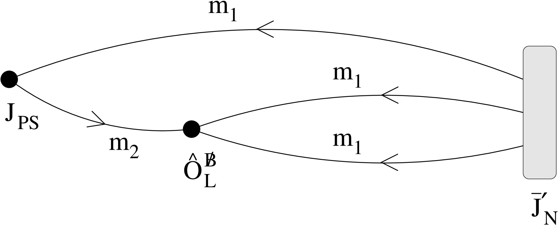
FIG. 2.: Quark flow diagram for the nucleon decay three point function with the mass assignment. Filled circles denote the local operators and shaded rectangular is for the smeared operator.

FIG. 3.: (a) Effective mass for the pion with $|{\vec{p}}|a=0$ at $K=0.15464$ and (b) effective energy for the pion with $|{\vec{p}}|a=\pi/14$ at $K=0.15620$. The pion correlation functions consist of the local sink and the wall source without gauge fixing. Solid lines denote the fitting results with an error band of one standard deviation obtained by global fits of the pion propagators.

FIG. 4.: Effective mass for the nucleon with the smeared source at (a) $K=0.15464$ and (b) $K=0.15620$. Solid lines denote the fitting results with an error band of one standard deviation obtained by global fits of the nucleon smeared-local propagators.

FIG. 5.: Effective mass for the nucleon with the local source at (a) $K=0.15464$ and (b) $K=0.15620$. Solid lines denote the fitting results with an error band of one standard deviation obtained by global fits of the nucleon smeared-local propagators.

FIG. 6.: Ratio $R^{\alpha\beta}(t)$ for (a) $\alpha$ and (b) $\beta$ parameters at $K=0.15620$. Solid lines denote the fitting results with an error band of one standard deviation.

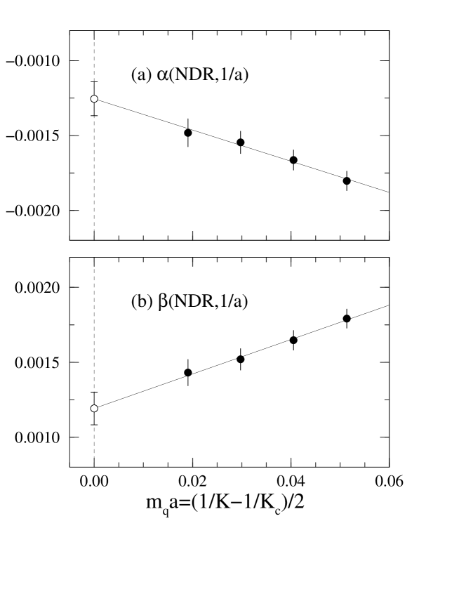
FIG. 7.: Chiral extrapolations of (a) $\alpha$ and (b) $\beta$ parameters. Solid lines denote linear fits.

FIG. 8.: Ratio $R(t,t^{\prime}=29)$ for the relevant form factor in $\langle\pi^{0}|(ud_{R})u_{L}|p\rangle$ at (a) $K=0.15464$ and (b) $K=0.15620$. Solid lines denote the fitting results with an error band of one standard deviation.

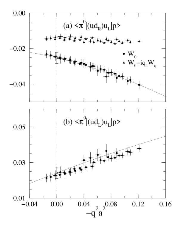
FIG. 9.: $-q^{2}a^{2}$ dependences for the relevant form factor $W_{0}$ in (a) $\langle\pi^{0}|(ud_{R})u_{L}|p\rangle$ and (b) $\langle\pi^{0}|(ud_{L})u_{L}|p\rangle$. Combination of form factors $W_{0}-iq_{4}W_{q}$ is also plotted in (a) for comparison. Solid lines denote the function $c_{0}+c_{1}\cdot(-q^{2}a^{2})+c_{2}\cdot(-q^{2}a^{2})^{2}$.

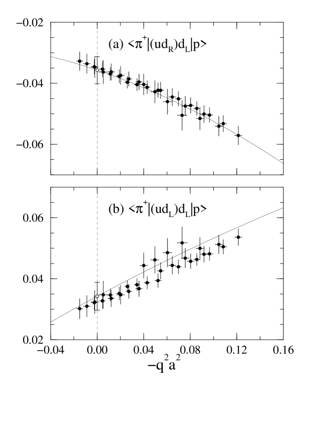
FIG. 10.: Same as Fig. 9 for (a) $\langle\pi^{+}|(ud_{R})d_{L}|p\rangle$ and (b) $\langle\pi^{+}|(ud_{L})d_{L}|p\rangle$.

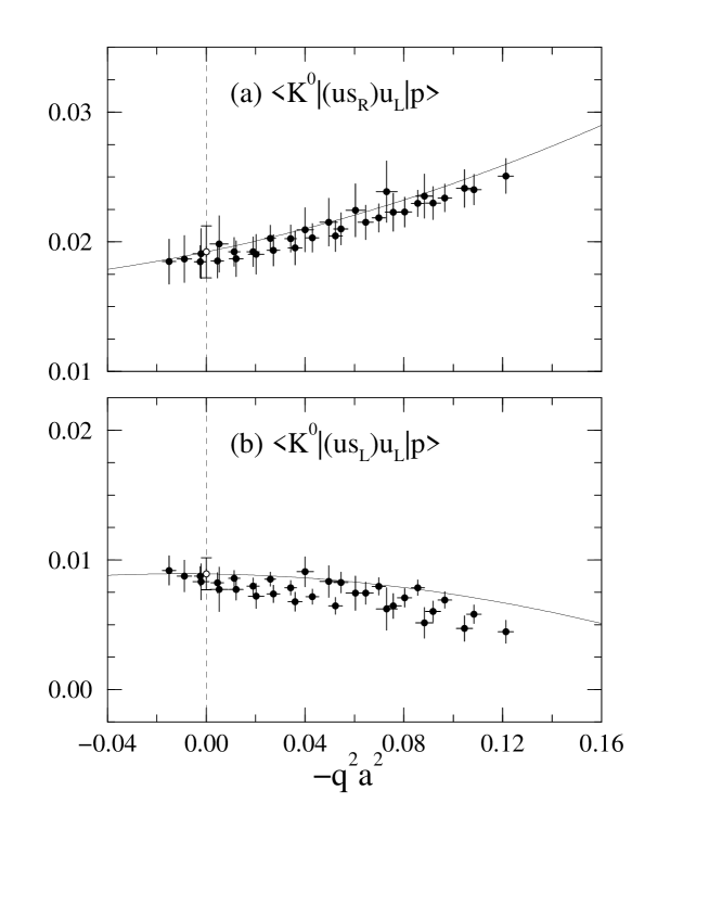
FIG. 11.: $-q^{2}a^{2}$ dependences for the relevant form factor $W_{0}$ in (a) $\langle K^{0}|(us_{R})u_{L}|p\rangle$ and (b) $\langle K^{0}|(us_{L})u_{L}|p\rangle$. Solid lines denote the function $c_{0}+c_{1}\cdot(-q^{2}a^{2})+c_{2}\cdot(-q^{2}a^{2})^{2}+c_{4}\cdot m_{s}a$.

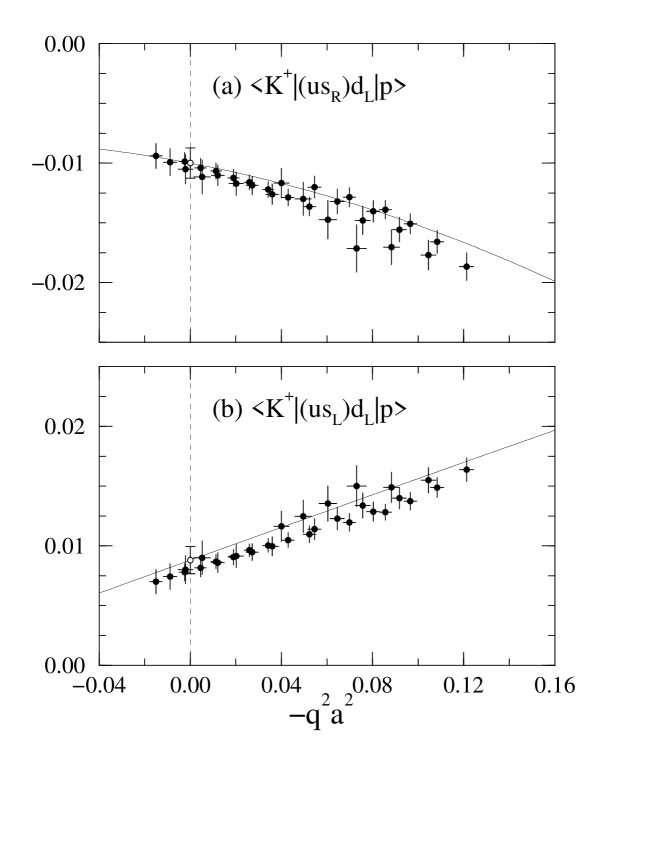
FIG. 12.: Same as Fig. 11 for (a) $\langle K^{+}|(us_{R})d_{L}|p\rangle$ and (b) $\langle K^{+}|(us_{L})d_{L}|p\rangle$.

FIG. 13.: Same as Fig. 11 for (a) $\langle K^{+}|(ud_{R})s_{L}|p\rangle$ and (b) $\langle K^{+}|(ud_{L})s_{L}|p\rangle$.

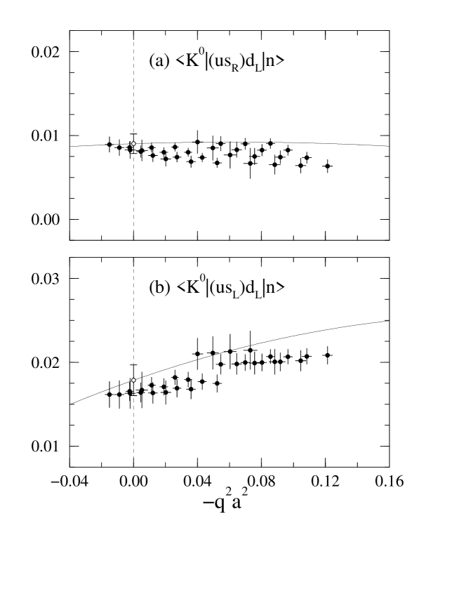
FIG. 14.: Same as Fig. 11 for (a) $\langle K^{0}|(us_{R})d_{L}|n\rangle$ and (b) $\langle K^{0}|(us_{L})d_{L}|n\rangle$.

FIG. 15.: Same as Fig. 9 for (a) $\langle\eta|(ud_{R})u_{L}|p\rangle$ and (b) $\langle\eta|(ud_{L})u_{L}|p\rangle$.

FIG. 16.: Comparison of relevant form factors with tree-level predictions of ChPT. Crosses denote the ChPT results with $|\alpha|=|\beta|=0.003$GeV³.

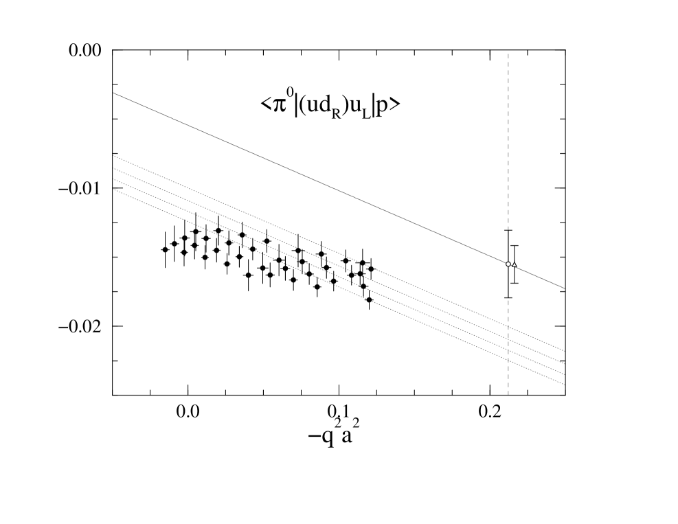
FIG. 17.: $W_{0}(q^{2})-iq_{4}W_{q}(q^{2})$ as a function of $-q^{2}a^{2}$. Dashed vertical line denote the soft pion limit $-q^{2}a^{2}=m_{N}^{2}a^{2}=(0.4607)^{2}$. See text for solid and dotted lines. Triangle denotes the results for $\alpha/(\surd 2f)$.

FIG. 18.: One-loop diagrams for (a) quark self energy and (b)$-$(d) vertex corrections for the three-quark operator. $p$ denotes a external quark momentum and $i$, $j$ and $k$ at the ends of quark lines label color indices.

TABLE I.: Hadron masses at $\beta=6.0$ in quenched QCD.

$K$	$m_{\pi}a$	$m_{\rho}a$	$m_{N}a$
0.15464	0.3209(8)	0.4350(22)	0.6674(38)
0.15516	0.2843(9)	0.4135(26)	0.6253(43)
0.15568	0.2436(9)	0.3925(33)	0.5814(52)
0.15620	0.1957(11)	0.3723(45)	0.5359(69)
0.157136(12)		0.3346(56)	0.4607(89)

TABLE II.: Four-momentum transfers from the nucleon at rest to the pseudoscalar meson. $E_{PS}$ is the energy of the pseudoscalar meson with spatial momentum ${\vec{p}}$.

		$|\vec{p}|a=0$	$|\vec{p}|a=\pi/24$		$|\vec{p}|a=\pi/14$
$K$ for $m_{1}$	$K$ for $m_{2}$	$-q^{2}a^{2}$	$E_{PS}\cdot a$	$-q^{2}a^{2}$	$E_{PS}\cdot a$	$-q^{2}a^{2}$
0.15464	0.15464	0.1200(28)	0.3467(10)	0.0857(26)	0.3912(12)	$0.0259(22)$
	0.15516		0.3302(11)	0.0966(27)	0.3767(13)	$0.0341(24)$
	0.15568		0.3131(12)	0.1084(29)	0.3619(15)	$0.0429(25)$
	0.15620		0.2953(14)	0.1213(31)	0.3469(21)	$0.0523(28)$
0.15516	0.15464		0.3304(10)	0.0698(27)	0.3769(13)	$0.0113(23)$
	0.15516	0.1163(31)	0.3132(11)	0.0803(29)	0.3620(14)	$0.0190(25)$
	0.15568		0.2953(13)	0.0918(30)	0.3469(15)	$0.0272(26)$
	0.15620		0.2765(15)	0.1045(32)	0.3316(22)	$0.0359(28)$
0.15568	0.15464		0.3138(11)	0.0545(29)	0.3626(14)	$-0.0025(24)$
	0.15516		0.2957(12)	0.0645(31)	0.3473(16)	$0.0045(26)$
	0.15568	0.1141(36)	0.2768(14)	0.0757(33)	0.3317(19)	$0.0120(28)$
	0.15620		0.2567(16)	0.0883(35)	0.3159(25)	$0.0202(31)$
0.15620	0.15464		0.2969(13)	0.0400(33)	0.3480(18)	$-0.0150(27)$
	0.15516		0.2777(14)	0.0495(36)	0.3322(19)	$-0.0089(29)$
	0.15568		0.2575(15)	0.0604(39)	0.3163(23)	$-0.0021(32)$
	0.15620	0.1158(47)	0.2356(18)	0.0730(42)	0.3003(31)	$0.0052(37)$

TABLE III.: Results for $\alpha$ and $\beta$ parameters as a function of quark mass. Operators are renormalized at the scale $\mu$ in the NDR scheme.

	$\alpha a^{3}$		$\beta a^{3}$
$K$	$\mu=1/a$	$\mu=\pi/a$	$\mu=1/a$	$\mu=\pi/a$
0.15464	$-0.00180(6)$	$-0.00207(7)$	0.00179(6)	0.00205(7)
0.15516	$-0.00166(7)$	$-0.00191(8)$	0.00165(7)	0.00189(8)
0.15568	$-0.00155(7)$	$-0.00177(8)$	0.00152(7)	0.00174(8)
0.15620	$-0.00148(9)$	$-0.00170(11)$	0.00143(9)	0.00164(10)
0.157136(12)	$-0.00125(11)$	$-0.00144(13)$	0.00119(11)	0.00137(12)

TABLE IV.: Comparison of $\alpha$ and $\beta$ parameters in lattice QCD. All calculations are done with the Wilson quark action in the quenched approximation. Lattice cutoff $a^{-1}$ is determined from $m_{\rho}$. Quark mass is defined by $m_{q}=\left(1/2K-1/2K_{c}\right)\cdot a^{-1}$.

Ref.	Hara et al. [2, 17]	Bowler et al. [3, 18]	Gavela et al. [4, 19]	This work
Lattice size	$16^{3}\times 48$	$8^{3}\times 16$	$10^{2}\times 20\times 40$	$28^{2}\times 48\times 80$
No. config.	15	32	30	100
$a^{-1}$ [GeV]	1.81(6)	1.45(9)	$2.2(4)$	$2.30(4)$
Spatial size [fm3]	$(1.7)^{3}$	$(1.1)^{3}$	$(0.9)^{2}\times 1.8$	$(2.4)^{2}\times 4.1$
Quark mass [MeV]	$109\hbox to0.0pt{\lower 3.5pt\hbox{$\mathchar 0\relax\sim$}\hss}\raise 1.0pt\hbox{$<$}m_{q}\hbox to0.0pt{\lower 3.5pt\hbox{$\mathchar 0\relax\sim$}\hss}\raise 1.0pt\hbox{$<$}696$	$184\hbox to0.0pt{\lower 3.5pt\hbox{$\mathchar 0\relax\sim$}\hss}\raise 1.0pt\hbox{$<$}m_{q}\hbox to0.0pt{\lower 3.5pt\hbox{$\mathchar 0\relax\sim$}\hss}\raise 1.0pt\hbox{$<$}477$	$82\hbox to0.0pt{\lower 3.5pt\hbox{$\mathchar 0\relax\sim$}\hss}\raise 1.0pt\hbox{$<$}m_{q}\hbox to0.0pt{\lower 3.5pt\hbox{$\mathchar 0\relax\sim$}\hss}\raise 1.0pt\hbox{$<$}223$	$44\hbox to0.0pt{\lower 3.5pt\hbox{$\mathchar 0\relax\sim$}\hss}\raise 1.0pt\hbox{$<$}m_{q}\hbox to0.0pt{\lower 3.5pt\hbox{$\mathchar 0\relax\sim$}\hss}\raise 1.0pt\hbox{$<$}118$
$\alpha$ [GeV3]		$|\alpha|\sim 0.065$	$|\alpha|=0.019(2)$	$\alpha=-0.015(1)$
$\beta$ [GeV3]	$|\beta|=0.029(6)$	$|\beta|\sim 0.050$		$\beta=0.014(1)$
Renorm. scheme		Pauli-Villars	DRED	NDR
Renorm. scale		$\mu=85$ GeV	$\mu=1/a$	$\mu=1/a$

TABLE V.: Results for relevant form factors in the independent nucleon decay matrix elements of eqs. (15)$-$(21). Operators are renormalized at the scale $\mu$ in the NDR scheme.

matrix element	$\mu=1/a$		$\mu=\pi/a$
	lattice units	GeV2	lattice units	GeV2
$\langle\pi^{0}|(ud_{R})u_{L}|p\rangle$	$-0.0253(31)$	$-0.134(16)$	$-0.0289(36)$	$-0.153(19)$
$\langle\pi^{0}|(ud_{L})u_{L}|p\rangle$	$0.0242(32)$	$0.128(17)$	$0.0278(37)$	$0.147(20)$
$\langle\pi^{+}|(ud_{R})d_{L}|p\rangle$	$-0.0357(45)$	$-0.189(24)$	$-0.0409(51)$	$-0.216(27)$
$\langle\pi^{+}|(ud_{L})d_{L}|p\rangle$	$0.0343(45)$	$0.181(24)$	$0.0394(52)$	$0.208(28)$
$\langle K^{0}|(us_{R})u_{L}|p\rangle$	$0.0192(20)$	$0.102(11)$	$0.0213(22)$	$0.113(12)$
$\langle K^{0}|(us_{L})u_{L}|p\rangle$	$0.0089(12)$	$0.0471(63)$	$0.0092(13)$	$0.0487(69)$
$\langle K^{+}|(us_{R})d_{L}|p\rangle$	$-0.0100(13)$	$-0.0529(69)$	$-0.0118(15)$	$-0.0624(79)$
$\langle K^{+}|(us_{L})d_{L}|p\rangle$	$0.0088(11)$	$0.0466(58)$	$0.0105(13)$	$0.0555(69)$
$\langle K^{+}|(ud_{R})s_{L}|p\rangle$	$-0.0248(27)$	$-0.131(14)$	$-0.0282(31)$	$-0.149(16)$
$\langle K^{+}|(ud_{L})s_{L}|p\rangle$	$0.0268(28)$	$0.142(15)$	$0.0304(32)$	$0.161(17)$
$\langle K^{0}|(us_{R})d_{L}|n\rangle$	$0.0090(12)$	$0.0476(63)$	$0.0094(13)$	$0.0497(69)$
$\langle K^{0}|(us_{L})d_{L}|n\rangle$	$0.0179(18)$	$0.0947(95)$	$0.0198(20)$	$0.105(11)$
$\langle\eta|(ud_{R})u_{L}|p\rangle$	$0.0007(11)$	$0.0037(58)$	$0.0004(12)$	$0.0021(63)$
$\langle\eta|(ud_{L})u_{L}|p\rangle$	$0.0191(25)$	$0.101(13)$	$0.0212(28)$	$0.112(15)$

REFERENCES

[1] See, e.g., S. J. Brodsky, J. Ellis, J. S. Hagelin
and C. T. Sachrajda,
Nucl. Phys. B238 (1984) 561.
[2] Y. Hara, S. Itoh, Y. Iwasaki and T. Yoshié,
Phys. Rev. D34 (1986) 3399.
[3] K. C. Bowler, D. Daniel, T. D. Kieu,
D. G. Richards and C. J. Scott,
Nucl. Phys. B296 (1988) 431.
[4] M. B. Gavela et al.,
Nucl. Phys. B312 (1989) 269.
[5] JLQCD Collaboration, N. Tsutsui et al.,
Nucl. Phys. B (Proc. Suppl.) 73 (1999) 297.
[6] S. Weinberg, Phys. Rev. Lett. 43 (1979) 1566;
F. Wilczek and A. Zee, Phys. Rev. Lett. 43 (1979) 1571.
[7] L. F. Abbott and M. B. Wise,
Phys. Rev. D22 (1980) 2208.
[8] M. Claudson, M. B. Wise and L. J. Hall,
Nucl. Phys. B195 (1982) 297.
[9] D. G. Richards, C. T. Sachrajda and C. J. Scott,
Nucl. Phys. B286 (1987) 683.
[10] P. B. Mackenzie, Nucl. Phys. B
(Proc. Suppl.) 30 (1993) 35;
A. S. Kronfeld, ibid.30 (1993) 445;
A. X. El-Khadra, A. S. Kronfeld and P. B. Mackenzie,
Phys. Rev. D55 (1997) 3933.
[11] G. P. Lepage and P. B. Mackenzie,
Phys. Rev. D48 (1993) 2250.
[12] R. Groot, J. Hoek and J. Smit,
Nucl. Phys. B237 (1984) 111.
[13] S. Chadha and M. Daniel,
Nucl. Phys. B229 (1983) 105.
[14] Particle Data Group,
Eur. Phys. J. C3 (1998) 1;
S. Y. Hsueh et al., Phys. Rev. D38 (1988) 2056.
[15] C. Bernard, T. Draper, G. Hockney and A. Soni, in
Lattice Gauge Theory: A Challenge in Large-Scale Computing,
eds. B. Bunk et al. (Plenum, New York, 1986);
G. W. Kilcup et al., Phys. Lett. 164B (1985) 347.
[16] C. T. H. Davies et al.,
Phys. Rev. D56 (1997) 2755.
[17] S. Itoh, Y. Iwasaki and T. Yoshié,
Phys. Lett. 183B (1987) 351.
[18] K. C. Bowler et al.,
Nucl. Phys. B240 [FS12] (1984) 213.
[19] G. Martinelli and C. T. Sachrajda,
Nucl. Phys. B316 (1989) 355.
[20] F. Butler, H. Chen, J. Sexton, A. Vaccarino and
D. Weingarten,
Nucl. Phys. B430 (1994) 179.
[21] T. Bhattacharya, R. Gupta, G. Kilcup and
S. Sharpe,
Phys. Rev. D53 (1996) 6486.
[22] J. F. Donoghue and E. Golowich,
Phys. Rev. D26 (1982) 3092.