DESY 99-170
Least-squares optimized polynomials for
fermion simulations

Abstract

Least-squares optimized polynomials are discussed which are needed in the two-step multi-bosonic algorithm for Monte Carlo simulations of quantum field theories with fermions. A recurrence scheme for the calculation of necessary coefficients in the recursion and for the evaluation of these polynomials is introduced.

1 Introduction

In popular Monte Carlo simulation algorithms for QCD and other similar quantum field theories the main difficulty is the evaluation of the determinant of the fermion action matrix. This can be achieved by stochastic procedures with the help of auxiliary bosonic “pseudofermion” fields.

In the two-step multi-bosonic (TSMB) algorithm [1] an approximation of the fermion determinant is achieved by the pseudofermion fields corresponding to a polynomial approximation of some negative power $x^{-\alpha}$ of the fermion matrix [2]. The auxiliary bosonic fields are updated according to the multi-bosonic action [3]. The error of the polynomial approximation is corrected in a global accept-reject decision by using better polynomial approximations. Sometimes a reweighting of gauge configurations in the evaluation of expectation values is also necessary. This can also be performed by high order polynomials.

The polynomials used in the TSMB algorithm have to approximate the function $x^{-\alpha}\bar{P}(x)$ in some non-negative interval $x\in[\epsilon,\lambda],\;0\leq\epsilon<\lambda$. Here $\bar{P}(x)$ is a known polynomial, typically another cruder approximation of $x^{-\alpha}$. The approximation scheme and optimization procedure can be chosen differently. The least-squares optimization [4] is an efficient and flexible possibility. (For other approximation schemes see [5, 6].)

In this review the basic relations for least-squares optimized polynomials are presented as introduced in [1, 2]. Particular attention is paid to a recurrence scheme which can be applied for determining the necessary high order polynomials and for evaluating them numerically. The details of the TSMB algorithm will not be considered. For a comprehensive summary and references see [7]. For experience on the application of TSMB in a recent large scale numerical simulation see [8, 9].

2 Basic relations

Least-squares optimization provides a general and flexible framework for obtaining the necessary optimized polynomials in multi-bosonic fermion algorithms. Here we introduce the basic formulae in the way it has been done in [2, 9].

We want to approximate the real function $f(x)$ in the interval $x\in[\epsilon,\lambda]$ by a polynomial $P_{n}(x)$ of degree $n$. The aim is to minimize the deviation norm

$$\delta_{n}\equiv\left\{N_{\epsilon,\lambda}^{-1}\;\int_{\epsilon}^{\lambda}dx\,w(x)^{2}\left[f(x)-P_{n}(x)\right]^{2}\right\}^{\frac{1}{2}}\ .$$ (1)

Here $w(x)$ is an arbitrary real weight function and the overall normalization factor $N_{\epsilon,\lambda}$ can be chosen by convenience, for instance, as

$$N_{\epsilon,\lambda}\equiv\int_{\epsilon}^{\lambda}dx\,w(x)^{2}f(x)^{2}\ .$$ (2)

A typical example of functions to be approximated is $f(x)=x^{-\alpha}/\bar{P}(x)$ with $\alpha>0$ and some polynomial $\bar{P}(x)$. The interval is usually such that $0\leq\epsilon<\lambda$. For optimizing the relative deviation one takes a weight function $w(x)=f(x)^{-1}$.

$\delta_{n}^{2}$ is a quadratic form in the coefficients of the polynomial which can be straightforwardly minimized. Let us now consider, for simplicity, only the relative deviation from the simple function $f(x)=x^{-\alpha}=w(x)^{-1}$. Let us denote the polynomial corresponding to the minimum of $\delta_{n}$ by

$$P_{n}(\alpha;\epsilon,\lambda;x)\equiv\sum_{\nu=0}^{n}c_{n\nu}(\alpha;\epsilon,\lambda)x^{n-\nu}\ .$$ (3)

Performing the integral in $\delta_{n}^{2}$ term by term we obtain

$$\delta_{n}^{2}=1-2\sum_{\nu=0}^{n}c_{\nu}V_{\nu}^{(\alpha)}+\sum_{\nu_{1},\nu_{2}=0}^{n}c_{\nu_{1}}M_{\nu_{1},\nu_{2}}^{(\alpha)}c_{\nu_{2}}\ ,$$ (4)

where

$$V_{\nu}^{(\alpha)}=\frac{\lambda^{1+\alpha+n-\nu}-\epsilon^{1+\alpha+n-\nu}}{(\lambda-\epsilon)(1+\alpha+n-\nu)}\ ,$$

$$M_{\nu_{1},\nu_{2}}^{(\alpha)}=\frac{\lambda^{1+2\alpha+2n-\nu_{1}-\nu_{2}}-\epsilon^{1+2\alpha+2n-\nu_{1}-\nu_{2}}}{(\lambda-\epsilon)(1+2\alpha+2n-\nu_{1}-\nu_{2})}\ .$$ (5)

The coefficients of the polynomial corresponding to the minimum of $\delta_{n}^{2}$, or of $\delta_{n}$, are

$$c_{\nu}\equiv c_{n\nu}(\alpha;\epsilon,\lambda)=\sum_{\nu_{1}=0}^{n}M_{\nu\nu_{1}}^{(\alpha)-1}V_{\nu_{1}}^{(\alpha)}\ .$$ (6)

The value at the minimum is

$$\delta_{n}^{2}\equiv\delta_{n}^{2}(\alpha;\epsilon,\lambda)=1-\sum_{\nu_{1},\nu_{2}=0}^{n}V_{\nu_{1}}^{(\alpha)}M_{\nu_{1},\nu_{2}}^{(\alpha)-1}V_{\nu_{2}}^{(\alpha)}\ .$$ (7)

The solution of the quadratic optimization in (6)-(7) gives in principle a simple way to find the required least-squares optimized polynomials. The practical problem is, however, that the matrix $M^{(\alpha)}$ is not well conditioned because it has eigenvalues with very different magnitudes. In order to illustrate this let us consider the special case $(\alpha=1,\;\lambda=1,\;\epsilon=0)$ with $n=10$. In this case the eigenvalues are:

$$0.4435021205e-14\ ,\hskip 5.0pt0.1045947635e-11\ ,\hskip 5.0pt0.1143819915e-9\ ,$$

$$0.7698917100e-8\ ,\hskip 10.00002pt0.3571195735e-6\ ,\hskip 10.00002pt0.1211873623e-4\ ,$$

$$0.3120413130e-3\ ,\hskip 10.00002pt0.6249495675e-2\ ,\hskip 10.00002pt0.9849331094e-1\ ,$$

$$1.075807246\ .$$ (8)

A numerical investigation shows that, in general, the ratio of maximal to minimal eigenvalues is of the order of ${\cal O}(10^{1.5n})$. It is obvious from the structure of $M^{(\alpha)}$ in (5) that a rescaling of the interval $[\epsilon,\lambda]$ does not help. The large differences in magnitude of the eigenvalues implies through (6) large differences of magnitude in the coefficients $c_{n\nu}$ and therefore the numerical evaluation of the optimal polynomial $P_{n}(x)$ for large $n$ is non-trivial.

Let us now return to the general case with arbitrary function $f(x)$ and weight $w(x)$. It is very useful to introduce orthogonal polynomials $\Phi_{\mu}(x)\;(\mu=0,1,2,\ldots)$ satisfying

$$\int_{\epsilon}^{\lambda}dx\,w(x)^{2}\Phi_{\mu}(x)\Phi_{\nu}(x)=\delta_{\mu\nu}q_{\nu}\ .$$ (9)

and expand the polynomial $P_{n}(x)$ in terms of them:

$$P_{n}(x)=\sum_{\nu=0}^{n}d_{n\nu}\Phi_{\nu}(x)\ .$$ (10)

Besides the normalization factor $q_{\nu}$ let us also introduce, for later purposes, the integrals $p_{\nu}$ and $s_{\nu}$ by

$$q_{\nu} \equiv \int_{\epsilon}^{\lambda}dx\,w(x)^{2}\Phi_{\nu}(x)^{2}\ ,$$

$$p_{\nu} \equiv \int_{\epsilon}^{\lambda}dx\,w(x)^{2}\Phi_{\nu}(x)^{2}x\ ,$$

$$s_{\nu} \equiv \int_{\epsilon}^{\lambda}dx\,w(x)^{2}x^{\nu}\ .$$ (11)

It can be easily shown that the expansion coefficients $d_{n\nu}$ minimizing $\delta_{n}$ are independent of $n$ and are given by

$$d_{n\nu}\equiv d_{\nu}=\frac{b_{\nu}}{q_{\nu}}\ ,$$ (12)

where

$$b_{\nu}\equiv\int_{\epsilon}^{\lambda}dx\,w(x)^{2}f(x)\Phi_{\nu}(x)\ .$$ (13)

The minimal value of $\delta_{n}^{2}$ is

$$\delta_{n}^{2}=1-N_{\epsilon,\lambda}^{-1}\sum_{\nu=0}^{n}d_{\nu}b_{\nu}\ .$$ (14)

Rescaling the variable $x$ by $x^{\prime}=\rho x$ allows for considering only standard intervals, say $[\epsilon/\lambda,1]$. The scaling properties of the optimized polynomials can be easily obtained from the definitions. Let us now again consider the simple function $f(x)=x^{-\alpha}$ and relative deviation with $w(x)=x^{\alpha}$ when the rescaling relations are:

$$\delta_{n}^{2}(\alpha;\epsilon\rho,\lambda\rho) = \delta_{n}^{2}(\alpha;\epsilon,\lambda)\ ,$$

$$P_{n}(\alpha;\epsilon\rho,\lambda\rho;x) = \rho^{-\alpha}P_{n}(\alpha;\epsilon,\lambda;x/\rho)\ ,$$

$$c_{n\nu}(\alpha;\epsilon\rho,\lambda\rho) = \rho^{\nu-n-\alpha}c_{n\nu}(\alpha;\epsilon,\lambda)\ .$$ (15)

In applications to multi-bosonic algorithms for fermions the decomposition of the optimized polynomials as a product of root-factors is needed. This can be written as

$$P_{n}(\alpha;\epsilon,\lambda;x)=c_{n0}(\alpha;\epsilon,\lambda)\prod_{j=1}^{n}[x-r_{nj}(\alpha;\epsilon,\lambda)]\ .$$ (16)

The rescaling properties here are:

$$c_{n0}(\alpha;\epsilon\rho,\lambda\rho) = \rho^{-n-\alpha}\,c_{n0}(\alpha;\epsilon,\lambda)\ ,$$

$$r_{nj}(\alpha;\epsilon\rho,\lambda\rho) = \rho\,r_{nj}(\alpha;\epsilon,\lambda)\ .$$ (17)

The root-factorized form (16) can also be used for the numerical evaluation of the polynomials with matrix arguments if a suitable optimization of the ordering of roots is performed [2].

The above orthogonal polynomials satisfy three-term recurrence relations which are very useful for numerical evaluation. In fact, at large $n$ the recursive evaluation of the polynomials is numerically more stable than the evaluation with root factors. For general $f(x)$ and $w(x)$, the first two ortogonal polynomials with $\mu=0,1$ are given by

$$\Phi_{0}(x)=1\ ,\hskip 20.00003pt\Phi_{1}(x)=x-\frac{s_{1}}{s_{0}}\ .$$ (18)

The higher order polynomials $\Phi_{\mu}(x)$ for $\mu=2,3,\ldots$ can be obtained from the recurrence relation

$$\Phi_{\mu+1}(x)=(x+\beta_{\mu})\Phi_{\mu}(x)+\gamma_{\mu-1}\Phi_{\mu-1}(x)\ ,\hskip 20.00003pt(\mu=1,2,\ldots)\ ,$$ (19)

where the recurrence coefficients are given by

$$\beta_{\mu}=-\frac{p_{\mu}}{q_{\mu}}\ ,\hskip 30.00005pt\gamma_{\mu-1}=-\frac{q_{\mu}}{q_{\mu-1}}\ .$$ (20)

Defining the polynomial coefficients $f_{\mu\nu}\;(0\leq\nu\leq\mu)$ by

$$\Phi_{\mu}(x)=\sum_{\nu=0}^{\mu}f_{\mu\nu}x^{\mu-\nu}$$ (21)

the above recurrence relations imply the normalization convention

$$f_{\mu 0}=1\ ,\hskip 30.00005pt(\mu=0,1,2,\ldots)\ .$$ (22)

The rescaling relations for the orthogonal polynomials easily follow from the definitions. For the simple function $f(x)=x^{-\alpha}$ and relative deviation with $w(x)=x^{\alpha}$ we have

$$\Phi_{\mu}(\alpha;\rho\epsilon,\rho\lambda;x)=\rho^{\mu}\,\Phi_{\mu}(\alpha;\epsilon,\lambda;x/\rho)\ .$$ (23)

For the quantities introduced in (2) this implies

$$q_{\nu}(\alpha;\rho\epsilon,\rho\lambda) = \rho^{2\alpha+1+2\nu}\,q_{\nu}(\alpha;\epsilon,\lambda)\ ,$$

$$p_{\nu}(\alpha;\rho\epsilon,\rho\lambda) = \rho^{2\alpha+2+2\nu}\,p_{\nu}(\alpha;\epsilon,\lambda)\ ,$$

$$s_{\nu}(\alpha;\rho\epsilon,\rho\lambda) = \rho^{2\alpha+1+\nu}\,s_{\nu}(\alpha;\epsilon,\lambda)\ .$$ (24)

For the expansion coefficients defined in (12)-(13) one obtains

$$b_{\nu}(\alpha;\rho\epsilon,\rho\lambda) = \rho^{\alpha+1+\nu}\,b_{\nu}(\alpha;\epsilon,\lambda)\ ,$$

$$d_{\nu}(\alpha;\rho\epsilon,\rho\lambda) = \rho^{-\alpha-\nu}\,d_{\nu}(\alpha;\epsilon,\lambda)\ ,$$ (25)

and the recurrence coefficients in (19)-(20) satisfy

$$\beta_{\mu}(\alpha;\rho\epsilon,\rho\lambda) = \rho\,\beta_{\mu}(\alpha;\epsilon,\lambda)\ ,$$

$$\gamma_{\mu-1}(\alpha;\rho\epsilon,\rho\lambda) = \rho^{2}\,\gamma_{\mu-1}(\alpha;\epsilon,\lambda)\ .$$ (26)

For general intervals $[\epsilon,\lambda]$ and/or functions $f(x)=x^{-\alpha}\bar{P}(x)$ the orthogonal polynomials and expansion coefficients have to be determined numerically. In some special cases, however, the polynomials can be related to some well know ones. An example is the weight factor

$$w^{(\rho,\sigma)}(x)^{2}=(x-\epsilon)^{\rho}(\lambda-x)^{\sigma}\ .$$ (27)

Taking, for instance, $\rho=2\alpha,\;\sigma=0$ this weight is similar to the one for relative deviation from the function $f(x)=x^{-\alpha}$, which would be just $x^{2\alpha}$. In fact, for $\epsilon=0$ these are exactly the same and for small $\epsilon$ the difference is negligible. The corresponding orthogonal polynomials are simply related to the Jacobi polynomials [9], namely

$$\Phi^{(\rho,\sigma)}_{\nu}(x)=(\lambda-\epsilon)^{\nu}\nu!\,\frac{\Gamma(\rho+\sigma+\nu+1)}{\Gamma(\rho+\sigma+2\nu+1)}P^{(\sigma,\rho)}_{\nu}\left(\frac{2x-\lambda-\epsilon}{\lambda-\epsilon}\right)\ .$$ (28)

Comparing different approximations with different $(\rho,\sigma)$ the best choice is usually $\rho=2\alpha,\;\sigma=0$ which corresponds to optimizing the relative deviation (see the appendix of [9]).

For large condition numbers $\lambda/\epsilon$ least-squares optimization is much better than the Chebyshev approximation used for the approximation of $x^{-1}$ in [3]. The Chebyshev approximation is minimizing the maximum of the relative deviation

$$R(x)\equiv xP(x)-1\ .$$ (29)

For the deviation norm

$$\delta_{max}\equiv\max_{x\in[\epsilon,\lambda]}|R(x)|$$ (30)

the least-squares approximation is slightly worse than the Chebyshev approximation. An example is shown by fig. 1. In the left lower corner the Chebyshev approximation has $Rc(0.0002)=-0.968$ compared to $Ro(0.0002)=-0.991$ for the least-squares optimization. For smaller condition numbers the Chebyshev approximation is not as bad as is shown by fig. 1. Nevertheless, in QCD simulations in sufficiently large volumes the condition number is of the order of the light quark mass squared in lattice units which can be as large as ${\cal O}(10^{6}-10^{7})$.

Figure  1 also shows that the least-squares optimization is quite good in the minimax norm in (30), too. It can be proven that

$$|Ro(\epsilon)|=\max_{x\in[\epsilon,\lambda]}\,|Ro(x)|$$ (31)

hence the minimax norm can also be easily obtained from

$$\delta_{max}^{(o)}=\max_{x\in[\epsilon,\lambda]}\,|Ro(x)|=|Ro(\epsilon)|\ .$$ (32)

Therefore the least squares-optimization is also well suited for controlling the minimax norm, if for some reason it is required.

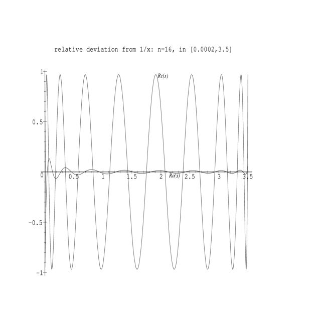
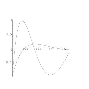
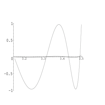
Figure 1: The comparison of the relative deviation $R(x)\equiv xP(x)-1$ for the Chebyshev polynomial $(Rc(x))$ and the quadratically optimized polynomial $(Ro(x))$. In the lower part the two ends of the interval are zoomed.

In QCD simulations the inverse power to be approximated ($\alpha$) is related to the number of Dirac fermion flavours: $\alpha=N_{f}/2$. If only $u$- and $d$-quarks are considered we have $N_{f}=2$ and the function to be approximated is $x^{-1}$. The dependence of the (squared) least-squares norm in (1) on the polynomial order $n$ is shown by fig. 2 for different values of the condition number $\lambda/\epsilon$. The dependence on $\alpha=N_{f}/2$ is illustrated by fig. 3.

Figure 2: The (squared) deviation norm $\delta^{2}$ of the polynomial approximations of $x^{-1}$ as function of the order for different values of $\lambda/\epsilon$. The asterisks show the $\epsilon/\lambda\to 0$ limit.

Figure 3: The (squared) deviation norm $\delta^{2}$ of the polynomial approximations of $x^{-\alpha}$ as function of the order at $\lambda/\epsilon=10^{5}$ for different values of $\alpha$.

Another possible application of least-squares optimized polynomials is the numerical evaluation of the zero mass lattice action proposed by Neuberger [10]. If one takes, for instance, the weight factor in (27) corresponding to the relative deviation, then the function $x^{-1/2}$ has to be expanded in the Jacobi polynomials $P^{(1,0)}$.

3 Recurrence scheme

The expansion in orthogonal polynomials is very useful because it allows for a numerically stable evaluation of the least-squares optimized polynomials by the recurrence relation (19). The orthogonal polynomials themselves can also be determined recursively.

A recurrence scheme for obtaining the recurrence coefficients $\beta_{\mu},\gamma_{\mu-1}$ and expansion coefficients $d_{\nu}=b_{\nu}/q_{\nu}$ has been given in [8, 7]. In order to obtain $q_{\nu},p_{\nu}$ contained in (20) one can use the relations

$$q_{\mu}=\sum_{\nu=0}^{\mu}f_{\mu\nu}s_{2\mu-\nu}\ ,\hskip 20.00003ptp_{\mu}=\sum_{\nu=0}^{\mu}f_{\mu\nu}\left(s_{2\mu+1-\nu}+f_{\mu 1}s_{2\mu-\nu}\right)\ .$$ (33)

The coefficients themselves can be calculated from $f_{11}=-s_{1}/s_{0}$ and (19) which gives

$$f_{\mu+1,1} = f_{\mu,1}+\beta_{\mu}\ ,$$

$$f_{\mu+1,2} = f_{\mu,2}+\beta_{\mu}f_{\mu,1}+\gamma_{\mu-1}\ ,$$

$$f_{\mu+1,3} = f_{\mu,3}+\beta_{\mu}f_{\mu,2}+\gamma_{\mu-1}f_{\mu-1,1}\ ,$$

$$\ldots$$

$$f_{\mu+1,\mu} = f_{\mu,\mu}+\beta_{\mu}f_{\mu,\mu-1}+\gamma_{\mu-1}f_{\mu-1,\mu-2}\ ,$$

$$f_{\mu+1,\mu+1} = \beta_{\mu}f_{\mu,\mu}+\gamma_{\mu-1}f_{\mu-1,\mu-1}\ .$$ (34)

The orthogonal polynomial and recurrence coefficients are recursively determined by (20) and (33)-(3). The expansion coefficients for the optimized polynomial $P_{n}(x)$ can be obtained from

$$b_{\mu}=\sum_{\nu=0}^{\mu}f_{\mu\nu}\int_{\epsilon}^{\lambda}dx\,w(x)^{2}f(x)x^{\mu-\nu}\ .$$ (35)

The ingredients needed for this recursion are the basic integrals $s_{\nu}$ defined in (2) and

$$t_{\nu}\equiv\int_{\epsilon}^{\lambda}dx\,w(x)^{2}f(x)x^{\nu}\ .$$ (36)

The recurrence scheme based on the coefficients of the orthogonal polynomials $f_{\mu\nu}$ in (3) is not optimal for large orders $n$, neither for arithmetics nor for storage requirements. A better scheme can be built up on the basis of the integrals

$$r_{\mu\nu}\equiv\int_{\epsilon}^{\lambda}dx\,w(x)^{2}\Phi_{\mu}(x)x^{\nu}\ ,$$

$$\mu=0,1,\ldots,n;\hskip 15.00002pt\nu=\mu,\mu+1,\ldots,2n-\mu\ .$$ (37)

The recurrence coefficients $\beta_{\mu},\;\gamma_{\mu-1}$ can be expressed from

$$q_{\mu}=r_{\mu\mu}\ ,\hskip 20.00003ptp_{\mu}=r_{\mu,\mu+1}+f_{\mu 1}r_{\mu\mu}$$ (38)

and eq. (20) as

$$\beta_{\mu}=-f_{\mu 1}-\frac{r_{\mu,\mu+1}}{r_{\mu\mu}}\ ,\hskip 20.00003pt\gamma_{\mu-1}=-\frac{r_{\mu\mu}}{r_{\mu-1,\mu-1}}\ .$$ (39)

It follows from the definition that

$$r_{0\nu} = \int_{\epsilon}^{\lambda}dx\,w(x)^{2}x^{\nu}=s_{\nu}\ ,$$

$$r_{1\nu} = \int_{\epsilon}^{\lambda}dx\,w(x)^{2}(x^{\nu+1}+f_{11}x^{\nu})=s_{\nu+1}+f_{11}s_{\nu}\ .$$ (40)

The recurrence relation (19) for the orthogonal polynomials implies

$$r_{\mu+1,\nu}=r_{\mu,\nu+1}+\beta_{\mu}r_{\mu\nu}+\gamma_{\mu-1}r_{\mu-1,\nu}\ .$$ (41)

This has to be supplemented by

$$f_{11}=-\frac{s_{1}}{s_{0}}$$ (42)

and by the first equation from (3):

$$f_{\mu+1,1}=f_{\mu,1}+\beta_{\mu}\ .$$ (43)

Eqs. (39)-(43) define a complete recurrence scheme for determining the orthogonal polynomials $\Phi_{\mu}(x)$. The moments $s_{\nu}$ of the integration measure defined in (2) serve as the basic input in this scheme.

The integrals $b_{\nu}$ in (13), which are necessary for the expansion coefficients $d_{\nu}$ in (12), can also be calculated in a similar scheme built up on the integrals

$$b_{\mu\nu}\equiv\int_{\epsilon}^{\lambda}dx\,w(x)^{2}f(x)\Phi_{\mu}(x)x^{\nu}\ ,$$

$$\mu=0,1,\ldots,n;\hskip 15.00002pt\nu=0,1,\ldots,n-\mu\ .$$ (44)

The relations corresponding to (3)-(41) are now

$$b_{0\nu}=\int_{\epsilon}^{\lambda}dx\,w(x)^{2}f(x)x^{\nu}=t_{\nu}\ ,$$ (45)

$$b_{1\nu}=\int_{\epsilon}^{\lambda}dx\,w(x)^{2}f(x)(x^{\nu+1}+f_{11}x^{\nu})=t_{\nu+1}+f_{11}t_{\nu}\ ,$$

$$b_{\mu+1,\nu}=b_{\mu,\nu+1}+\beta_{\mu}b_{\mu\nu}+\gamma_{\mu-1}b_{\mu-1,\nu}\ .$$

The only difference compared to (3)-(41) is that the moments of $w(x)^{2}$ are now replaced by the ones of $w(x)^{2}f(x)$.

It is interesting to collect the quantities which have to be stored in order that the recurrence can be resumed. This is useful if after stopping the iterations, for some reason, the recurrence will be restarted. Let us assume that the quantities $q_{\nu}\;(\nu=0,\ldots,n)$, $b_{\nu}\;(\nu=0,\ldots,n)$, $\beta_{\nu}\;(\nu=1,\ldots,n-1)$ and $\gamma_{\nu}\;(\nu=0,\ldots,n-2)$ are already known and one wants to resume the recurrence in order to calculate these quantities for higher indices. For this it is enough to know the values of

$$f_{n-1,1}\ ,\;\;r_{n-1,n-1}\ ,$$

$$R^{(0)}_{0\ldots n}\equiv(r_{0,2n+1},r_{1,2n},\ldots,r_{n,n+1})\ ,$$

$$R^{(1)}_{0\ldots n}\equiv(r_{0,2n},r_{1,2n-1},\ldots,r_{n,n})\ ,$$

$$B^{(1)}_{0\ldots n}\equiv(b_{0,n},b_{1,n-1},\ldots,b_{n,0})\ ,$$

$$B^{(2)}_{0\ldots n-1}\equiv(b_{0,n-1},b_{1,n-2},\ldots,b_{n-1,0})\ .$$ (46)

This shows that for maintaining a resumable recurrence it is enough to store a set of quantities linearly increasing in $n$.

An interesting question is the increase of computational load as a function of the highest required order $n$. At the first sight this seems to go just like $n^{2}$, which is surprising because, as eq. (6) shows, finding the minimum requires the inversion of an $n\otimes n$ matrix. However, numerical experience shows that the number of required digits for obtaining a precise result does also increase linearly with $n$. This is due to the linearly increasing logarithmic range of eigenvalues, as illustrated by (2). Using, for instance, Maple V for the arbitrary precision arithmetic, the computation slows down by another factor going roughly as (but somewhat slower than) $n^{2}$. Therefore, the total slowing down in $n$ is proportional to $n^{4}$. For the same reason the storage requirements increase by $n^{2}$.

4 A convenient choice for TSMB

In the TSMB algorithm for Monte Carlo simulations of fermionic theories, besides the simple function $x^{-\alpha}$, also the function $x^{-\alpha}/\bar{P}(x)$ has to be approximated. Here $\bar{P}(x)$ is typically a lower order approximation to $x^{-\alpha}$. In this case, if one chooses to optimize the relative deviation, the basic integrals defined in (2) and (36) are, respectively,

$$s_{\nu} = \int_{\epsilon}^{\lambda}dx\,\bar{P}(x)^{2}x^{2\alpha+\nu}\ ,$$

$$t_{\nu} = \int_{\epsilon}^{\lambda}dx\,\bar{P}(x)x^{\alpha+\nu}\ .$$ (47)

It is obvious that, if the recurrence coefficients for the expansion of the polynomial $\bar{P}(x)$ in orthogonal polynomials are known, the recursion scheme can also be used for the evaluation of $s_{\nu}$ and $t_{\nu}$.

Another observation is that the integrals in (4) can be simplifyed if, instead of choosing the weight factor $w(x)^{2}=\bar{P}(x)^{2}x^{2\alpha}$, one takes

$$w(x)^{2}=\bar{P}(x)x^{\alpha}\ ,$$ (48)

which leads to

$$s_{\nu} = \int_{\epsilon}^{\lambda}dx\,\bar{P}(x)x^{\alpha+\nu}\ ,$$

$$t_{\nu} = \int_{\epsilon}^{\lambda}dx\,x^{\nu}\ .$$ (49)

Since $\bar{P}(x)$ is an approximation to $x^{-\alpha}$, the function $f(x)\equiv x^{-\alpha}/\bar{P}(x)$ is close to one and the difference between $f(x)^{-2}$ and $f(x)^{-1}$ is small. Therefore the least-squares optimized approximations with the weights $w(x)^{2}=f(x)^{-2}$ and $w(x)^{2}=f(x)^{-1}$ are also similar. It turns out that the second choice is, in fact, a little bit better because the largest deviation from $x^{-\alpha}$ typically occurs at the lower end of the interval $x=\epsilon$ where $\bar{P}(x)$ is smaller than $x^{-\alpha}$. As a consequence, $\bar{P}(x)x^{\alpha}<1$ and $\bar{P}(x)x^{\alpha}>\bar{P}(x)^{2}x^{2\alpha}$. This means that choosing the weight factor in (48) is emphasising more the lower end of the interval where $\bar{P}(x)$ as an approximation of $x^{-\alpha}$ is worst.

In summary: least-squares optimization is a flexible and powerful tool which can serve as a basis for applying the two-step multi-bosonic algorithm for Monte Carlo simulations of QCD and other similar theories. With the help of the recurrence scheme described in the previous section one can determine the necessary polynomial approximations to high enough orders.

References

- [1] Montvay, I.: An algorithm for gluinos on the lattice. Nucl. Phys. B466 (1996) 259–284
- [2] Montvay, I.: Quadratically optimized polynomials for fermion simulations. Comput. Phys. Commun. 109 (1998) 144–160
- [3] Lüscher, M.: A new approach to the problem of dynamical quarks in numerical simulations of lattice QCD. Nucl. Phys. B418 (1994) 637–648
- [4] Rivlin, T.J.: An Introduction to the Approximation of Functions, Blaisdell Publ. Company, 1969.
- [5] Wolff, U.: Multiboson simulation of the Schrödinger functional. Nucl. Phys. Proc. Suppl. 63 (1998) 937-939
- [6] de Forcrand, P.: UV-filtered fermionic Monte Carlo. Nucl. Phys. Proc. Suppl. 73 (1999) 822-824; also see this Proceedings.
- [7] Montvay, I.: Multi-bosonic algorithms for dynamical fermion simulations. Workshop on Molecular Dynamics on Parallel Computers, Jülich, Germany, February 1999, to appear in the proceedings; hep-lat/9903029.
- [8] Kirchner, R. et al.: Evidence for discrete chiral symmetry breaking in N=1 supersymmetric Yang-Mills theory. Phys. Lett. B446 (1999) 209–215
- [9] Campos, I. et al.: Monte Carlo simulation of SU(2) Yang-Mills theory with light gluinos. Eur. Phys. J. C; DOI 10.1007/s100529900183.
- [10] Neuberger, H.: Exactly massless quarks on the lattice. Phys. Lett. B417 (1998) 141–144.