November 1999

The Phase Diagram and Spectrum of Gauge-Fixed

Abelian Lattice Gauge Theory

Wolfgang Bock^#, Ka Chun Leung^%

Institute of Physics, University of Siegen, 57068 Siegen, Germany

Maarten F.L. Golterman^$

Department of Physics, Washington University St. Louis, MO 63130, USA

Yigal Shamir^&

Beverly and Raymond Sackler Faculty of Exact Sciences, Tel-Aviv University,

Ramat Aviv 69978, Israel

Abstract

We consider a lattice discretization of a covariantly gauge-fixed abelian gauge theory. The gauge fixing is part of the action defining the theory, and we study the phase diagram in detail. As there is no BRST symmetry on the lattice, counterterms are needed, and we construct those explicitly. We show that the proper adjustment of these counterterms drives the theory to a new type of phase transition, at which we recover a continuum theory of (free) photons. We present both numerical and (one-loop) perturbative results, and show that they are in good agreement near this phase transition. Since perturbation theory plays an important role, it is important to choose a discretization of the gauge-fixing action such that lattice perturbation theory is valid. Indeed, we find numerical evidence that lattice actions not satisfying this requirement do not lead to the desired continuum limit.

While we do not consider fermions here, we argue that our results, in combination with previous work, provide very strong evidence that this new phase transition can be used to define abelian lattice chiral gauge theories.

^# e-mail: bock@physik.uni-siegen.de
^% e-mail: leung@physik.uni-siegen.de
^$ e-mail: maarten@aapje.wustl.edu
^& e-mail: shamir@post.tau.ac.il

1 Introduction

In this paper we continue our investigation of the gauge-fixing approach to the construction of lattice chiral gauge theories. In this approach, gauge invariance is broken both through the gauge-fixing terms and through the fermions. This requires adding a complete set of counterterms to the theory, in addition to the gauge-fixing terms, and these counterterms will need to be tuned. Showing that this can be done corresponds to demonstrating that the phase diagram contains a continuous phase transition which can be employed to construct the desired continuum chiral gauge theory [1, 2].

Here, we will restrict ourselves to the abelian case. This avoids many of the subtle questions concerning Gribov copies which arise in the non-abelian case. In particular, it makes it possible to drop the ghost sector from consideration [3], while still testing many of the key elements in this approach to lattice chiral gauge theories.

We will employ (a generalization of) the lattice gauge-fixing action proposed in Ref. [4]. Since we wish to maintain close contact with standard weak-coupling perturbation theory, we consider a lattice version of the Lorentz gauge. (Other gauges may work as well, but we believe that it is important to restrict oneself to a renormalizable gauge.) On the lattice, i.e. in the regulated theory, there is no gauge or BRST symmetry, and both the transverse gauge fields and the fermions will couple to the gauge degrees of freedom, represented by the longitudinal part of the gauge field.

This leads to the following simple questions, both of which can be addressed without simulating the full theory including all its dynamical degrees of freedom: 1) when we turn off the transverse part of the gauge field, do we obtain a theory of free (chiral) fermions in the correct representation of the gauge group (in the abelian case, with the correct charges), decoupled from the longitudinal modes? and 2) when we turn off the fermions, do we obtain a theory of free photons, again decoupled from the longitudinal degrees of freedom?

It is well known that (most) small perturbations of the gauge-invariant compact lattice formulation of a U(1) gauge theory do not change the nature of its (weak-coupling) continuum limit (they correspond to irrelevant directions) [5]. However, previous work has shown that it is generically not possible to construct chiral gauge couplings near such a continuum limit (for reviews, see Refs. [6, 7]). In our approach, gauge fixing plays an essential role in the construction of the theory. This means that the coupling in front of the gauge-fixing action has to be large enough to bring us to a new type of continuous phase transition in the phase diagram, at which both questions above can be answered affirmatively.

We have addressed question 1) in previous work [8, 9, 10, 11, 12]. We showed that, in the “reduced” model, in which only the fermions and the longitudinal gauge fields are kept, indeed a new type of phase transition occurs. At this phase transition, a continuum limit can be defined in which free chiral fermions with the correct charges emerge, decoupled from these longitudinal degrees of freedom. Here, we address the second question. We turn off the fermions, and we ask whether this new phase transition survives when the transverse degrees of freedom are present, and in particular, whether it allows us to construct a theory of free photons at the transition. We would like to emphasize that, even though, without fermions, this is not a new continuum theory, our critical point corresponds to a new type of universality class. This is the key element that allows us to couple fermions chirally to the gauge fields, without running into the problems which made many previous attempts unsuccessful.

In addition to this fundamental question, we also address a more technical issue. It was argued in Ref. [2] that one has to be very careful with the precise definition of the lattice version of the gauge-fixing action. A naive “standard” discretization of the Lorentz gauge-fixing action $(1/2\xi)\int d^{4}x\;(\partial\cdot A)^{2}$ will lead to the occurrence of a dense set of lattice Gribov copies (with no continuum counterpart). This corresponds to a large class of uncontrolled, rough fluctuations in the lattice theory, and may well spoil the existence of the critical point we are after. The lattice gauge-fixing action proposed in Ref. [4] does not suffer from this problem, and it is this action that we have used in our previous work. Here, we introduce a one-parameter class of lattice gauge-fixing actions, which interpolates between the naive discretization and the one of Ref. [4]. This corresponds to adding a direction to the phase diagram, and we explore the dependence of the phase structure on this new direction.

The organization of this paper is as follows. In Sect. 2 we give the full action for a gauge-fixed U(1) gauge theory, including a complete set of counterterms. In particular, we introduce the parameter $\widetilde{r}$, which interpolates between the naive gauge-fxing action and that of Ref. [4], and we discuss the above mentioned lattice Gribov copies. We argue that standard lattice perturbation theory should be valid as long as $\widetilde{r}$ is large enough. In Sect. 3 we present analytic results in preparation of a high-statistics numerical study of this model. We first explain the nature of the new phase transition (which we will denote as the “FM-FMD transition”) from the classical potential, and then provide a simple-minded mean-field analysis of the model. Since there is good qualitative agreement between mean field and our numerical results, we also give an overview of the structure of the phase diagram at this stage. We end this section with a calculation of the one-loop lattice photon propagator, and use it to determine some of the counterterms at one loop. We also consider a (composite) scalar two-point function. Then, in Sect. 4, we present our numerical results, which constitute the main part. First we discuss in detail how we determined the phase diagram. After that, we compute vector and scalar two-point functions numerically, and compare them with perturbation theory in order to determine whether we do indeed obtain a theory of free photons at the FM-FMD transition. Finally, we summarize and discuss our findings in the last section. There are two appendices, containing various technical details.

We would like to end this section with mentioning that, recently, a gauge-invariant construction of (anomaly-free) abelian chiral gauge theories on the lattice has been proposed, based on a Dirac operator satisfying the Ginsparg–Wilson relation [13] (for the non-abelian case, see Ref. [14]). The problems with the violation of gauge invariance discussed above do not apply in this case (they might if a gauge non-invariant approximation of the Dirac operator is used, however). An essential ingredient is that the fermion measure includes a gauge-field dependent phase factor which is determined by requiring the theory to be gauge invariant and local. Sofar, however, no explicit expression of the fermion measure was given, making this approach as yet not suitable for a numerical investigation.

2 The Model

The central idea of the gauge-fixing approach is to control the gauge degrees of freedom by a gauge-fixing procedure. The starting point is the gauge-fixed action in the continuum, the “target theory.” Correlation functions of the target theory in the continuum satisfy Slavnov–Taylor identities, as a consequence of the gauge symmetry. For an abelian gauge group, which will be the subject of this paper, the target action in the continuum is of the form,

$$S_{\rm c}=S_{{\rm c,G}}(A_{\mu})+S_{\rm c,F}(A_{\mu};\psi_{L},\psi_{R})+S_{{\rm c,g.f.}}(A_{\mu})\;,$$ (2.1)

where $S_{{\rm c,G}}(A_{\mu})={1\over 4}\int d^{4}x\,F_{\mu\nu}^{2}$ designates the gauge action, $S_{\rm c,F}(A_{\mu};\psi_{L},\psi_{R})$ is the chiral fermion action, and $S_{{\rm c,g.f.}}(A_{\mu})$ the gauge-fixing action. Here, we will consider the Lorentz gauge, which is renormalizable, and therefore allows us to study the (relevant part of the) phase diagram in perturbation theory. No ghosts are needed in the abelian case, and henceforth we will not introduce any ghosts on the lattice either [3]. We then have

$$S_{{\rm c,g.f.}}(A_{\mu})\!\! = \!\!\frac{1}{2\xi}\int d^{4}x\left(\sum_{\mu}\partial_{\mu}A_{\mu}\right)^{2}\;,$$ (2.2)

where $\xi$ is the gauge-fixing parameter. The goal is now to transcribe the target theory defined by the action (2.1) to the lattice using compact lattice link variables and the Haar measure as integration measure in the path integral.

The fermion action leads to violations of the Slavnov–Taylor identities if we use any one of the standard lattice fermion formulations, such as Wilson, staggered or domain-wall fermions, which are in conflict with chiral gauge invariance. Moreover, we will consider a class of gauge-fixing terms, dependent on a continuous parameter $\widetilde{r}$. They will lead to additional violations of the Slavnov–Taylor identities. The Slavnov–Taylor identities are restored in the continuum limit by adding a finite number of counterterms to the action, and appropriately tuning their coefficients [1] in the continuum limit.

In this paper, we will drop the fermion sector and, as mentioned in Sect. 1, focus on the question whether the lattice discretization of the target action with U(1) symmetry provides a valid formulation of a theory of free photons on the lattice. The lattice action is formulated in terms of the compact link variables $U_{\mu x}=\exp(iagA_{\mu x})$, with $g$ the gauge coupling and $a$ the lattice spacing (which we will set to one throughout this paper). The lattice action is then given by the expression

$$S=S_{\rm G}(U)+S_{{\rm g.f.}}(U)+S_{{\rm c.t.}}(U)\;.$$ (2.3)

where $S_{\rm G}(U)$ is the gauge action, $S_{{\rm g.f.}}(U)$ the gauge fixing, and $S_{{\rm c.t.}}(U)$ the counterterm action on the lattice. For the lattice transcription of the gauge action $S_{{\rm c,G}}(A_{\mu})$ we employed the standard plaquette action,

$$S_{{\rm G}}(U)=\frac{1}{g^{2}}\;\sum_{x}\sum_{\mu<\nu}\left\{1-\mbox{Re }U_{\mu\nu x}\right\}\;,$$ (2.4)

where $U_{\mu\nu x}=U_{\mu x}U_{\nu x+\hat{\mu}}U^{\dagger}_{\mu x+\hat{\nu}}U^{\dagger}_{\nu x}$ is the usual lattice plaquette variable. The lattice transcription of the gauge-fixing action is more subtle. A naive lattice discretization of Eq. (2.2) leads to

$$S_{{\rm g.f.}}^{\rm naive}(U)=\widetilde{\kappa}\;\sum_{x}\left(\sum_{\mu}\Delta^{-}_{\mu}V_{\mu x}\right)^{2}\;,$$ (2.5)

where

$$V_{\mu x}=\mbox{Im }U_{\mu x}\;,$$ (2.6)

$$\widetilde{\kappa}=\frac{1}{2g^{2}\xi}\;,$$ (2.7)

and $\Delta_{\mu}^{-}V_{\mu x}=V_{\mu x}-V_{\mu x-\hat{\mu}}$ ($\Delta_{\mu}^{-}$ is the backward nearest-neighbor lattice derivative). The problem with the naive lattice discretization is that the classical vacuum of the action $S_{{\rm G}}(U)+S_{{\rm g.f.}}^{\rm naive}(U)$ is not unique [2]. It is easy to see that $S_{{\rm G}}(U)+S_{{\rm g.f.}}^{\rm naive}(U)$ has absolute minima for a dense set of lattice Gribov copies $U_{\mu x}=g_{x}\;1\;g_{x+\hat{\mu}}^{\dagger}$, of the classical vacuum $U_{\mu x}=1$ for particular sets of $g_{x}$. An example of such lattice Gribov copies is displayed in Fig. 1,

Figure 1: Example of a lattice Gribov copy. Shown is only a two-dimensional projection of the four-dimensional lattice. The $U_{\mu x}$ fields on all the links attached to $x=x_{0}$ (fat lines) are equal to $-1$ and all other $U_{\mu x}$ fields are equal to one.

where we set $g_{x}=-1$ at site $x=x_{0}$ and $g_{x}=+1$ at all sites $x\neq x_{0}$. The $U_{\mu x}$ fields on the links attached to the site $x_{0}$ (fat lines) are equal to $-1$ whereas the $U_{\mu x}$ fields on all other links (thin lines) are equal to $+1$. These lattice Gribov copies are a high momentum lattice artifact with no counterpart in the continuum. (They should not be confused with continuum Gribov copies, which are a long-distance phenomenon.) It is clear that perturbation theory around only one of the absolute minima of $S_{\rm G}(U)+S^{\rm naive}_{\rm g.f.}(U)$, in particular the classical vacuum $U_{\mu x}=1$, may not give a valid description of the theory, and the phase diagram could (and will) turn out very different from what one would expect from naive perturbation theory.

It is however possible to remove the unwanted lattice Gribov copies of the classical vacuum (and therefore, by continuity, of field configurations perturbatively close to the vacuum) by adding a higher dimensional operator to the gauge-fixing action in Eq. (2.5). This procedure is similar to Wilson’s idea of removing the species doublers of the naive lattice fermion action by adding an operator of dimension larger than four (the Wilson term). Such higher dimensional operators do not affect the small-momentum behavior of the theory, but can be used to change the behavior at large momenta.

The gauge-fixing action we will use in this paper is given by the expression

$$S_{{\rm g.f.}}(U)=S_{{\rm g.f.}}^{\rm naive}(U)+\widetilde{r}\;\widetilde{\kappa}\;\sum_{x}\left\{\mbox{{\small$\frac{1}{4}$}}\;\left(C_{x}+C_{x}^{\dagger}\right)^{2}-B_{x}^{2}\right\}\;,$$ (2.8)

where

$$C_{x}=\sum_{y}\Box_{xy}(U)\;,$$ (2.9)

$$B_{x}=\sum_{\mu}\left(\frac{V_{\mu x-\hat{\mu}}+V_{\mu x}}{2}\right)^{2}\;,$$ (2.10)

and

$$\Box(U)_{xy}=\sum_{\mu}\left\{U_{\mu x}\;\delta_{x+\hat{\mu},y}+U_{\mu x-\hat{\mu}}^{\dagger}\;\delta_{x-\hat{\mu},y}-2\;\delta_{x,y}\right\}$$ (2.11)

is the covariant lattice Laplacian. In Eq. (2.8) we have multiplied the higher dimensional operator by a new parameter $\widetilde{r}$ which can be viewed as the analog of the Wilson parameter $r$ that multiplies the Wilson term. It can be shown that the action $S_{{\rm G}}(U)+S_{{\rm g.f.}}(U)$ has, for $\widetilde{r}>0$, a unique absolute minimum at $U_{\mu x}=1$ [4] so that, for $\widetilde{r}>0$, standard perturbation theory in $g$ is valid. The gauge-fixing action provides a continuous interpolation between the naive gauge-fixing action (2.5) ($\widetilde{r}=0$) and the gauge-fixing action at $\widetilde{r}=1$ which was introduced previously in Ref. [4] and was used in Refs. [8, 9, 10, 11, 12, 15].

We will study the $\widetilde{r}$ dependence of the phase diagram of the purely bosonic theory, and explore the effects of the lattice Gribov copies on the phase structure. Obviously, lattice Gribov copies introduce rough gauge degrees of freedom. It is therefore conceivable that lattice Gribov copies at small $\widetilde{r}$ give rise to a disordered or symmetric phase. It has been argued earlier that a chiral gauge theory cannot be obtained in such a phase [16]. This would teach us that, in the gauge-fixing approach to lattice chiral gauge theories, one needs to choose $\widetilde{r}$ of order one.

Finally, we have to specify the counterterm action. It contains all relevant and marginal operators which are allowed by the exact lattice symmetries [1]. In the case of the U(1) gauge theory there are six such terms:

$$S_{{\rm c.t.}}(U)\!\! = \!\!-\kappa\sum_{\mu x}\left\{U_{\mu x}+U_{\mu x}^{\dagger}\right\}-\;\lambda_{1}\;\sum_{x}\sum_{\mu\nu}\left(\Delta_{\nu}^{-}\;\mbox{Im }U_{\mu x}\right)^{2}$$ (2.12)

$$- \!\!\lambda_{2}\;\sum_{x}\sum_{\mu}\left(\Delta_{\mu}^{-}\mbox{Im }U_{\mu x}\right)^{2}-\lambda_{3}\;\sum_{x}\left(\sum_{\mu}\Delta_{\mu}^{-}\mbox{Im }U_{\mu x}\right)^{2}$$

$$- \!\!\lambda_{4}\;\sum_{x}\left(\sum_{\mu}(\mbox{Im }U_{\mu x})^{2}\right)^{2}-\lambda_{5}\;\sum_{x}\sum_{\mu}\left(\mbox{Im }U_{\mu x}\right)^{4}\;.$$

The term proportional to $\kappa$ is a mass counterterm for the gauge field. It is the only dimension-two counterterm. All other counterterms are of dimension four. An expansion in $g$ shows that the counterterms with coefficients $\lambda_{1}$, $\lambda_{2}$ and $\lambda_{3}$ are wave-function renormalization counterterms. The terms with the coefficients $\lambda_{4}$ and $\lambda_{5}$ are, to leading order in $g$, quartic in the gauge potential, and are needed to eliminate photon self-interactions. The coefficients of the counterterms have to be tuned such that the Slavnov–Taylor identities are satisfied in the continuum limit (cf. Sect. 3.3). Note that terms such as $\sum_{x}\sum_{\mu}(\Delta_{\mu}^{-}\mbox{Im }U_{\mu x})\sum_{\nu}(\mbox{Im }U_{\nu x})^{2}$ do not occur because of the symmetry $U_{\mu x}\to U^{\dagger}_{\mu x}$. However, such counterterms will have to be considered once the theory is coupled to fermions.

The path integral is defined by

$$Z\!\! = \!\!\int DU\;\exp(-S(U))$$ (2.13)

$$= \!\!\int DUD\phi\;\exp(-S(\phi_{x}^{\dagger}U_{\mu x}\phi_{x+\hat{\mu}}))\;,$$ (2.14)

where the action $S(U)$ is given in Eq. (2.3), and the integration over the link variables is performed with the usual Haar measure. Only the gauge action in Eq. (2.3) is invariant under the local gauge transformation

$$U_{\mu x}\rightarrow U_{\mu x}^{g}=g_{x}U_{\mu x}g_{x+\hat{\mu}}^{\dagger}\;.$$ (2.15)

In Eq. (2.14) we made the integration over the longitudinal gauge degrees of freedom $\phi_{x}$ explicit. It is easy to see that Eq. (2.13) follows from Eq. (2.14) by performing the gauge transformation (2.15) with $g_{x}=\phi^{\dagger}_{x}$ and using the fact that $\int D\phi=1$ [5]. The longitudinal modes can be viewed as group-valued Higgs fields $\phi_{x}$. We will therefore denote in the following $S(\phi_{x}^{\dagger}U_{\mu x}\phi_{x+\hat{\mu}})$ as the action in the “Higgs picture” and $S(U)$ as the action in the “vector picture.” Both pictures are equivalent and every observable in the vector picture has, according to Eq. (2.15), a counterpart in the Higgs picture. The path integral in the Higgs picture is invariant under the local transformation

$$\phi_{x}\rightarrow h_{x}\phi_{x}\;,\;\;\;\;U_{\mu x}\rightarrow h_{x}U_{\mu x}h_{x+\hat{\mu}}^{\dagger}\;.$$ (2.16)

Finally, we mention here that in $d$ space-time dimensions the path integrals (2.13) and (2.14) are invariant under the additional discrete symmetry (with all $\lambda_{i}=0$)

$$U_{\mu x}\rightarrow-U_{\mu x}\;,\;\;\;\;\;\kappa\rightarrow-\kappa-8\;d\;\widetilde{\kappa}\;\widetilde{r}\;,\;\;\;\;\;\widetilde{\kappa}\rightarrow\widetilde{\kappa}\;,\;\;\;\;\;\widetilde{r}\rightarrow\widetilde{r}\;,\;\;\;\;\;g\rightarrow g\;,\$$ (2.17)

which implies that we can restrict ourselves to the $\kappa>-4d\widetilde{\kappa}\widetilde{r}$ region of the $(\kappa,\widetilde{\kappa},\widetilde{r})$ phase diagram. In the following we will refer to

$$\kappa=-4d\widetilde{\kappa}\;\widetilde{r}$$ (2.18)

as the symmetry surface, or symmetry line (point) if $\widetilde{\kappa}$ or (and) $\widetilde{r}$ are kept fixed.

At $\widetilde{\kappa}=0$ and $\lambda_{i}=0$, $i=1,\ldots,5$, the model reduces to the U(1) gauge-Higgs model with group-valued Higgs fields. The resulting $(\kappa,g)$ phase diagram corresponds to the $\widetilde{\kappa}=0$ hyperplane of the four-dimensional $(\kappa,g,\widetilde{\kappa},\widetilde{r})$ phase diagram (for $\widetilde{\kappa}=0$ the model is independent of $\widetilde{r}$). In the limit $g\rightarrow 0$ the phase diagram of the gauge-Higgs model reduces to that of the four-dimensional XY model. This phase diagram of the XY model contains three phases: a ferromagnetic (FM) or broken phase at $\kappa>\kappa_{\rm FM-PM}\approx 0.15$, a paramagnetic (PM) or symmetric phase at $-\kappa_{\rm FM-PM}\leq\kappa\leq\kappa_{\rm FM-PM}$, and an antiferromagnetic (AM) phase at $\kappa<-\kappa_{\rm FM-PM}$. The $\kappa>0$ region is mapped by the symmetry (2.17) into the $\kappa<0$ region. This implies that the FM phase is mapped into the AM phase and vice versa. The FM-PM transition, and, because of the symmetry (2.17), also the PM-AM phase transition are second-order phase transitions. At $g>0$ the FM phase turns into a Higgs and the PM phase into a Coulomb phase, which we will still denote as FM and PM phases, respectively. There is strong evidence that also the FM-PM phase transition at $g>0$ is of second order [17]. The spectrum in the FM phase contains a massive vector boson with quantum numbers $J^{\rm PC}=1^{--}$ and a massive Higgs boson with quantum numbers $J^{\rm PC}=0^{++}$. The masses of both particles are expected to scale when $\kappa$ is tuned towards the second-order FM-PM phase transition. The spectrum in the Coulomb phase contains only a massless photon if one keeps away from the FM-PM phase transition [18]. The model in the Coulomb phase provides a valid formulation of free photons on the lattice but, as we explained before, because of the strongly fluctuating longitudinal gauge modes, it is not possible to formulate a chiral gauge theory with a gauge non-invariant fermion action in that phase. The spectrum near the FM-PM phase transition contains, apart from the massless photon, also positronium-like bound states of scalars [18]. At large $g$ and small $\kappa$ the phase diagram contains a confining (CF) phase, which is separated from the PM phase by a phase transition, located at $g\approx 1$.

In Refs. [8, 9, 10, 11, 12], we have studied the U(1) model with $\lambda_{i}=0$, $i=1,\ldots,5$ in the reduced limit where the gauge coupling is tuned to zero, while keeping $\widetilde{\kappa}=1/(2g^{2}\xi)$ fixed (reduced model). In this limit the transverse gauge degrees of freedom are gone and only the dynamics of the longitudinal gauge degrees of freedom remains. The path integral of this reduced model is given by Eq. (2.14) with all link variables set equal to one. The phase diagram of the reduced model at $\widetilde{r}=1$ contains, apart from the FM and PM phases, also a new type ferromagnetic directional (FMD) phase where the vector field $\mbox{Im}\,\phi_{x}^{\dagger}\phi_{x+\hat{\mu}}$ condenses and hypercubic rotation invariance on the lattice is broken (cf. the $\widetilde{r}=1$ plane of Fig. 6, which is very similar to the $\widetilde{r}=1$ reduced-model phase diagram).

The phase transition between the FM and FMD phases, which, as we will see, is also present in the full U(1) model, plays a crucial role in the gauge-fixing approach. While the photon is massive in the FM phase, one obtains a massless photon by tuning $\kappa$, from within the FM phase, towards this FM-FMD phase transition. Tuning all other counterterms as well should then lead to a theory of free, relativistic photons. We should note here that $\kappa$ is the only relevant counterterm parameter, whereas all the $\lambda_{i}$ are marginal. We therefore may expect that only $\kappa$ needs to be tuned nonperturbatively, while, with a given numerical precision, a one-loop, or even tree-level determination of the $\lambda_{i}$ will suffice. Indeed, the results which we will present in the following sections provide evidence of this.

With chiral fermions, we demonstrated that, in the reduced limit, the fermion spectrum contains only the desired chiral states [10, 11, 12].

The phase diagram at small $g$ is expected to look similar to the phase diagram of the reduced model, since the transverse components of the gauge fields are still very small. We will show in the following sections that even at a relatively large value of $g$ ($g=0.6$) the phase diagram is qualitatively very similar to the one for the reduced model, if $\widetilde{r}\approx 1$.

3 Analytical results

In this section we present our analytical results. Subsect. 3.1 deals with the constant-field approximation, which already gives some insight into the phase structure. In Subsect. 3.2 we will determine the $(\kappa,\widetilde{\kappa},\widetilde{r})$ phase diagram at fixed small $g$ in the mean-field approximation. The counterterm coefficients $\kappa$, $\lambda_{1}$, $\lambda_{2}$ and $\lambda_{3}$ are calculated to one-loop order in perturbation theory in Subsect. 3.3. In Subsect. 3.4 we analyze the spectrum near the FM-FMD phase transition in perturbation theory.

3.1 Constant-field approximation

In the constant-field approximation we set

$$U_{\mu x}=\exp(igA_{\mu})\;,$$ (3.1)

where $A_{\mu}$ is a space-time-independent vector potential. After inserting (3.1) into Eq. (2.3) all terms which contain derivatives of the gauge field vanish, and we obtain an expression for the classical potential density. Expanding the resulting expression in powers of $g$, we find

$$V_{{\rm cl}}(A_{\mu})\!\! = \!\!\kappa\left\{g^{2}\sum_{\mu}A_{\mu}^{2}+\ldots\right\}+\mbox{{\normalsize$\frac{1}{2}$}}\;g^{6}\;\widetilde{\kappa}\;\widetilde{r}\;\left\{\left(\sum_{\mu}A_{\mu}^{2}\right)\left(\sum_{\mu}A_{\mu}^{4}\right)+\ldots\right\}$$ (3.2)

$$\!\!-\lambda_{4}\;g^{4}\;\left\{\left(\sum_{\mu}A_{\mu}^{2}\right)^{2}+\ldots\right\}-\lambda_{5}\;g^{4}\;\left\{\sum_{\mu}A_{\mu}^{4}+\ldots\right\}\;,$$

where “$\ldots$” represents terms which are of higher order in $g^{2}$. A massless non-interacting photon is obtained for $\kappa=0$, $\lambda_{4}=0$ and $\lambda_{5}=0$. The relation $\kappa=\kappa_{\rm FM-FMD}=0$ defines a critical surface in the three-dimensional $(\kappa,\widetilde{\kappa},\widetilde{r})$ phase diagram where the photon mass vanishes. We will see later that the critical coupling $\kappa_{{\rm FM-FMD}}(\widetilde{\kappa},\widetilde{r})$ is shifted away from zero by perturbative corrections.

The minimization of the classical potential density (3.2) for $\lambda_{4}=\lambda_{5}=0$ shows that

$$\begin{array}[]{ll}\langle g\;A_{\mu}\rangle=0\;,&\mbox{for }\kappa\geq\kappa_{{\rm FM-FMD}}\;,\\ \langle g\;A_{\mu}\rangle=\pm\left(|\kappa-\kappa_{{\rm FM-FMD}}|/(6\;\widetilde{\kappa}\;\widetilde{r})\right)^{1/4}\;,&\mbox{for }\kappa<\kappa_{{\rm FM-FMD}}\;,\end{array}$$ (3.3)

for $\mu=1,\ldots,4$ (see Ref. [4], which also deals with the case $\lambda_{4}\neq 0$, $\lambda_{5}\neq 0$). This implies that $\kappa=\kappa_{{\rm FM-FMD}}=0$ corresponds to a phase transition between the FM phase where $\langle A_{\mu}\rangle$ vanishes and the gauge boson has a nonzero mass, and the FMD phase with a nonvanishing vector condensate $\langle A_{\mu}\rangle$. The hypercubic rotation invariance on the lattice is broken in the FMD phase by the nonvanishing vector condensate.

The constant-field approximation is supposed to provide a satisfactory description of the model only at large $\widetilde{\kappa}\sim 1/g^{2}$, where strongly fluctuating gauge configurations are suppressed by a small Boltzmann weight and the smoother gauge configurations are well approximated by a constant field. Indeed, as we will see, a perturbative expansion starting from the constant-field approximation can be developed by expanding $U_{\mu x}={\rm exp}(igA_{\mu x})$ and setting $\widetilde{\kappa}=1/(2\xi g^{2})$, with $\xi$ fixed. The situation is different at small $\widetilde{\kappa}$ where rough longitudinal fields are not sufficiently suppressed. This picture is confirmed by our previous investigation of the reduced model at $\widetilde{r}=1$, where we find indeed a FM-FMD phase transition at large $\widetilde{\kappa}$ (consistent with the constant field-approximation), but an FM-PM phase transition at small $\widetilde{\kappa}$. The emergence of the disordered PM phase at small $\widetilde{\kappa}$ is due to the dominance of rough gauge field configurations. Equation (3.2) shows that the classical potential density depends only on the product $\widetilde{\kappa}\widetilde{r}$. This suggests that a small value of $\widetilde{r}$ has the same effect as a small value of $\widetilde{\kappa}$ and that the “small $\kappa$”-region around $\widetilde{r}=0$ might indeed be filled with a PM phase. This conjecture will be confirmed by our mean-field analysis and Monte Carlo simulations.

3.2 Mean Field Calculation of the Phase diagram

In the following we set again $\lambda_{i}=0$, $i=1,\ldots,5$ and determine the phase boundaries in the $(\kappa,\widetilde{\kappa},\widetilde{r})$ space. The mean-field analysis for gauge theories on the lattice is ambiguous as it is in conflict with local gauge invariance [19]. For gauge-Higgs models the mean-field calculation in the vector picture leads to a wrong phase structure at small values of $\kappa$, whereas the mean-field approximation in the Higgs picture leads to a phase diagram which, at least qualitatively, complies at small $\kappa$ with Monte Carlo simulations. Since we are interested in the phase diagram at small $\kappa$, we performed our mean-field analysis in the Higgs picture. Here, we will only describe the results, while relegating all the technicalities to Appendix A.

All the results we are going to present in the following were obtained at $g=0.6$, scanning the three-dimensional $(\kappa,\widetilde{\kappa},\widetilde{r})$ phase diagram at $g=0.6$ by keeping either $\widetilde{\kappa}$ or $\widetilde{r}$ fixed. (We also performed a few scans of the four-dimensional $(g,\kappa,\widetilde{\kappa},\widetilde{r})$ parameter space in the $g$ direction at $\widetilde{r}=1$, $\kappa=0$ and several values of $\widetilde{\kappa}$ and find that the transition to the confining phase occurs always at values of $g$ which are larger than $0.6$.) The resulting two-dimensional sections through the $(\kappa,\widetilde{\kappa},\widetilde{r})$-phase diagram are displayed in the left columns of Figs. 2-5. The corresponding phase diagrams obtained from the Monte Carlo simulations are displayed in the right columns. They will be discussed in more detail in Sect. 4.1 but a first glimpse shows that they are, in most cases, similar to the mean-field phase diagrams.

The dash-dotted lines in Figs. 2-5 mark the symmetry line (2.18); we only determined the phase diagram above that line. The error bars in the mean-field phase diagrams mark the distance between two successive points in our scans of the phase diagram (cf. Appendix A).

Figs. 2a and b show the $(\kappa,\widetilde{\kappa})$ phase diagram at $\widetilde{r}=1$. There is a PM phase for small $|\widetilde{\kappa}|$ and small $|\kappa|$, and for large $\widetilde{\kappa}$ there is a phase-transition line separating an FM and an FMD phase. The plots in Figs. 2-3 show that the situation remains qualitatively the same when $\widetilde{r}$ is lowered. The phase diagram at $\widetilde{r}=0$ contains at small $\widetilde{\kappa}$ and $\kappa$ a PM phase, as for $\widetilde{r}>0$. The mean-field calculation, however, predicts that, at $\widetilde{r}=0$, the region at large $\widetilde{\kappa}$ and small $|\kappa|$ is filled by an FMD phase, which is in conflict with our Monte Carlo simulations (plot in the right column), which show that the PM phase extends to very large $\widetilde{\kappa}$ with no sign of an FMD phase. We therefore believe that the FMD phase at large $\widetilde{\kappa}$ is an artifact of the mean-field approximation (which tends to favor ordered over disordered phases). Figures 4-5 show three $(\kappa,\widetilde{r})$ phase-diagram plots at fixed $\widetilde{\kappa}$ values. The phase diagrams at $\widetilde{\kappa}=0.05$ and $0.2$ look very similar to those at fixed $\widetilde{r}>0$. For $\widetilde{\kappa}<0<\widetilde{r}$ or $\widetilde{r}<0<\widetilde{\kappa}$ we find an FM-AM phase transition which coincides with the symmetry line, Eq. (2.18). Figure 5 shows again that the mean-field calculation at $\widetilde{\kappa}=0.8$ does not lead to a PM phase at small $\widetilde{r}$.

We have compiled the Monte Carlo results for the $(\kappa,\widetilde{\kappa},\widetilde{r})$ phase diagram into a schematic graph, shown in Fig. 6. The FMD phase at large $\widetilde{\kappa}$ and $\widetilde{r}=0$ is not shown in that graph since, as we said, there is no evidence from Monte Carlo simulations that the FMD extends down to $\widetilde{r}=0$. Fig. 6 shows that the FM-PM and FM-FMD phase-transition sheets are separated by a tricritical line where three phases (FM, PM and FMD) meet; we will call this the FM-FMD-PM line. Similarly, also the FM-PM and FM-AM phase transition sheets are separated by an FM-AM-PM tricritical line (not shown in Fig. 6). The projections of these tricritical lines onto a constant-$\kappa$ plane are shown in Fig. 7a (mean field) and in Fig. 7b (Monte Carlo). We see that the discrepancy between the mean field and Monte Carlo results at $\widetilde{r}=0$ correlates with the fact that the mean-field and Monte Carlo locations of these tricritical lines differ slightly. In mean field, the PM phase ends at $\widetilde{\kappa}\approx 0.3$, and the FM-FMD-PM and FM-AM-PM lines merge into an FM-FMD-AM tricritical line, whose projection approaches the $\widetilde{r}=0$ axis for $\widetilde{\kappa}=\infty$.

In the mean-field approximation we find that the FM-PM transition is second order at $\widetilde{\kappa}=0$ (this is the “standard” gauge-Higgs model). It is still second order at $\widetilde{\kappa}>0$ and $\widetilde{r}=1$, but changes into a first order phase transition when $\widetilde{r}$ is lowered. Similarly we find that the FM-FMD transition is of second order at $\widetilde{r}=1$, but of first order at small $\widetilde{r}$. The FM-AM phase transition is always of first order.

Figure 2: The $(\kappa,\widetilde{\kappa})$ phase diagrams at $\widetilde{r}=1$ (Figs. a and b) and $\widetilde{r}=0.2$ (Figs. c and d). The plots on the left were obtained by a mean-field calculation, and those on the right by Monte Carlo simulations on a $4^{4}$ lattice. The dash-dotted lines mark the symmetry line (cf. Eq. (2.18)). The perturbative result for the FM-FMD transitions is represented in the plots on the right by solid lines. The relation between the perturbative and Monte Carlo results will be discussed in Sect. 4.1.

Figure 3: Same as Fig. 2, but for $\widetilde{r}=0.1$ (Figs. a and b) and $0$ (Figs. c and d). Note that the symmetry line in Figs. c and d coincides with the $\kappa=0$ axis.

Figure 4: The $(\kappa,\widetilde{r})$ phase diagrams for $\widetilde{\kappa}=0.05$ (Figs. a and b) and $0.2$ (Figs. c and d). The mean-field phase diagrams are displayed again on the left, and those from the Monte Carlo simulations on the right. The dash-dotted line is the symmetry line. The perturbative result for the FM-FMD transitions is represented in the plots on the right by solid lines. The relation between the perturbative and Monte Carlo results will be discussed in Sect. 4.1.

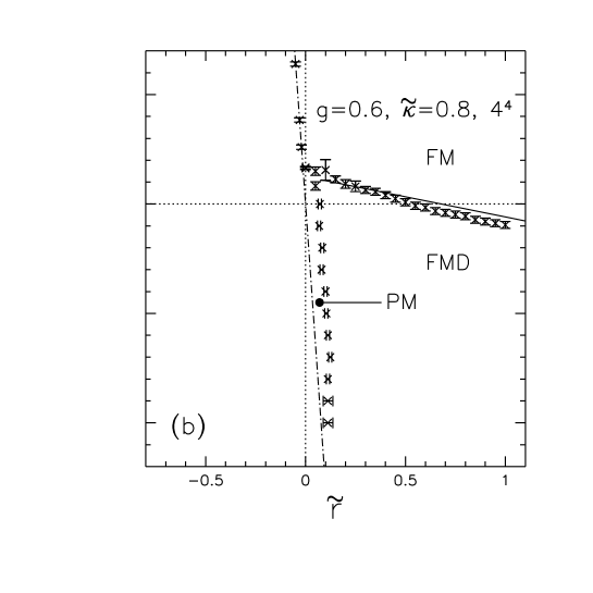
Figure 5: Same as Fig. 4 but for $\widetilde{\kappa}=0.8$.

3.3 Perturbative determination of the counterterm coefficients

The counterterm coefficients $\kappa$, $\lambda_{1}+\lambda_{3}$ and $\lambda_{2}$ can be calculated order by order in perturbation theory by demanding the Slavnov–Taylor identity

$$\sum_{\mu\nu}p_{\mu}\;q_{\nu}\;\langle A_{\mu}(p)\;A_{\nu}(q)\rangle=\xi\;\delta(p+q)$$ (3.4)

to be satisfied in the continuum limit $a\rightarrow 0$. (The Slavnov–Taylor identity does not determine the other linear combination, $\lambda_{1}-\lambda_{3}$, because it corresponds to a gauge-invariant operator.)

First, we transcribe the left-hand side of eq. (3.4) to a finite lattice,

$$W(p)=\sum_{\mu\nu}\widehat{p}_{\mu}\;\widehat{p}_{\nu}\;\Delta_{\mu\nu}^{V}(p)\;,$$ (3.5)

where $\widehat{p}_{\mu}=2\sin(p_{\mu}/2)$ is the lattice momentum, and

$$\Delta_{\mu\nu}^{V}(p)=\frac{1}{g^{2}\;L^{3}\;T}\left\langle\sum_{x,y}\mbox{Im}\;U_{\mu x}\;\mbox{Im}\;U_{\nu y}\exp(i\;p\;(x-y))\right\rangle\;.$$ (3.6)

is the vector two-point function in momentum space, with $L^{3}T$ the lattice volume of a cylindrical lattice of spatial extent $L$ and temporal extent $T$. The vector propagator $\Delta_{\mu\nu}^{V}(p)$ is now computed to a given order in $g^{2}$. The resulting expression for $\Delta_{\mu\nu}^{V}(p)$, and hence also for $W(p)$, will be a function of the counterterm coefficients.

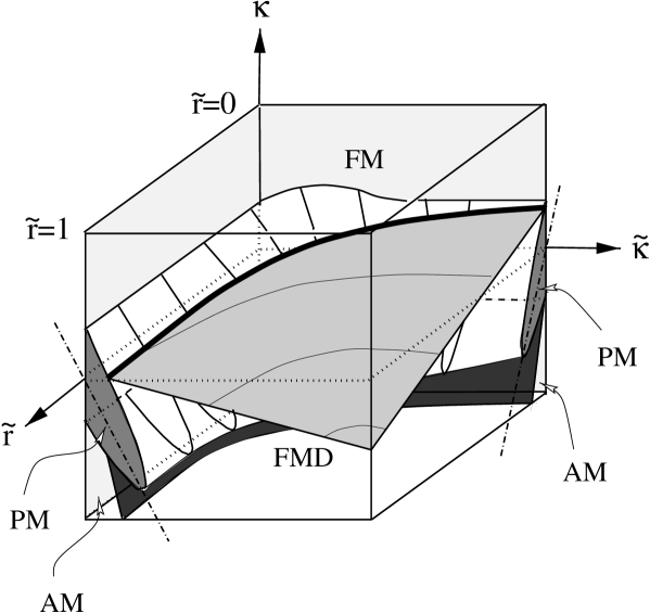
Figure 6: Schematic three-dimensional plot of the $(\kappa,\widetilde{\kappa},\widetilde{r})$ phase diagram in the range from $\widetilde{r}=0$ to $\widetilde{r}=1$, $\widetilde{\kappa}=0$ to $\widetilde{\kappa}=1$. The two dashed lines on the front faces of the phase diagram cube indicate the position of the symmetry surface (Eq. 2.18) on those faces. The thick line represents the FM-FMD-PM tricritical line.

The counterterm coefficients are then determined such that in the continuum limit

$$\lim_{a\rightarrow 0}W(p)=\xi$$ (3.7)

(keeping the physical volume fixed). Similarly, the coefficients $\lambda_{4}$ and $\lambda_{5}$ of the quartic counterterms can be calculated by requiring the Slavnov–Taylor identity

$$\sum_{\mu\nu\rho\sigma}p_{\mu}q_{\nu}k_{\rho}l_{\sigma}\;\langle A_{\mu}(p)A_{\nu}(q)A_{\rho}(k)A_{\sigma}(l)\rangle$$

$$=\xi^{2}\left(\delta(p+q)\;\delta(k+l)+\delta(p+k)\;\delta(q+l)+\delta(p+l)\;\delta(q+k)\right)\;$$ (3.8)

to be satisfied in the continuum limit $a\rightarrow 0$.

After inserting

$$A_{\mu x}=\widetilde{\sum_{p}}\exp\left(i\;p\cdot x\right)\;\exp\left(i\;p_{\mu}/2\right)\;A_{\mu}(p)\;,$$ (3.9)

with $\widetilde{\sum}_{p}=(L^{3}T)^{-1}\sum_{p}$, into the action (2.3), we obtain from the term bilinear in vector potential $A_{\mu}(p)$ for the tree-level vector propagator

$$\Delta^{V,(0)}_{\mu\nu}(p)=\left[\left(\widehat{p}^{2}+m^{2}\right)\;\delta_{\mu\nu}-\left(1-\frac{1}{\xi}\right)\;\widehat{p}_{\mu}\;\widehat{p}_{\nu}\right]^{-1}\;,\\$$ (3.10)

where

$$m^{2}=2\kappa g^{2}\;.$$ (3.11)

We included the mass counterterm in the tree-level propagator, since it also functions as an infrared cutoff.

Figure 7: Projection of the FM-FMD-PM and FM-AM-PM tricritical lines onto a $\kappa=\mbox{const}$ plane obtained by a mean-field calculation (Fig. a) and by a Monte Carlo simulation (Fig. b). The FM-FMD-PM and FM-AM-PM tricritical lines in Fig. a appear to merge into an FM-FMD-AM tricritical line at large $\widetilde{\kappa}$. The two solid curves in Fig. b are to guide the eye.

We have calculated the critical values of the coefficients $\kappa$, $\lambda_{1}$, $\lambda_{2}$ and $\lambda_{3}$ to one-loop order in perturbation theory. To one-loop order the vector propagator is

$$\Delta^{V,(1)}_{\mu\nu}(p)\!\! = \!\!Z_{\mu\nu}(g^{2})\;\left[\phantom{\left(\frac{1}{\xi}\right)}\!\!\!\!\!\!\!\!\!\!\!\!\left(m^{2}+(1+\lambda_{1}\;g^{2})\;\widehat{p}^{2}+\lambda_{2}\;g^{2}\;\widehat{p}_{\mu}^{2}\right)\;\delta_{\mu\nu}\right.$$ (3.12)

$$- \!\!\left.\left(1-\frac{1}{\xi}-\lambda_{3}\;g^{2}\right)\;\widehat{p}_{\mu}\;\widehat{p}_{\nu}+\Sigma_{\mu\nu}^{\rm bare}(p)\right]^{-1}\;,$$

with

$$Z_{\mu\nu}(g^{2})=1-g^{2}\;\mbox{{\normalsize$\frac{1}{2}$}}\;\widetilde{\sum_{k}}\left(\Delta_{\mu\mu}^{V,(0)}(k)+\Delta_{\nu\nu}^{V,(0)}(k)\right)\;,$$ (3.13)

and

$$\!\!\!\!\!\!\Sigma_{\mu\nu}^{\rm bare}(p)\!\! = \!\!\Sigma^{\rm g.f.}_{\mu\nu}(p)+\Sigma^{\rm G}_{\mu\nu}(p)\;,$$ (3.14)

$$\!\!\!\!\!\!\Sigma^{\rm g.f.}_{\mu\nu}(p)\!\! = \!\!\frac{2\;g^{2}}{\xi}\;\left[\mbox{{\small$\frac{1}{4}$}}\;\widetilde{r}\;\widetilde{\sum_{k}}\sum_{\alpha}\Delta_{\alpha\alpha}^{V,(0)}(k)\;\widehat{k}^{2}_{\alpha}+\mbox{{\small$\frac{1}{4}$}}\;\widetilde{r}\;\widehat{p}^{2}_{\mu}\;\widetilde{\sum_{k}}\sum_{\alpha}\Delta_{\alpha\alpha}^{V,(0)}(k)\;\cos^{2}(k_{\alpha}/2)\right.$$ (3.15)

$$\!\!\left.-\mbox{{\normalsize$\frac{1}{2}$}}\;\widetilde{\sum_{k}}\sum_{\alpha}\Delta_{\alpha\mu}^{V,(0)}(k)\;\widehat{k}_{\alpha}\;\widehat{k}_{\mu}\right]\;\delta_{\mu\nu}$$

$$\!\!-\frac{g^{2}}{\xi}\;\left[\widetilde{\sum_{k}}\;\Delta_{\mu\mu}^{V,(0)}(k)-\mbox{{\small$\frac{1}{4}$}}\;\widetilde{r}\;\widetilde{\sum_{k}}\;\Delta_{\mu\nu}^{V,(0)}(k)\;\widehat{k}_{\mu}\;\widehat{k}_{\nu}\right]\;\widehat{p}_{\mu}\;\widehat{p}_{\nu}\;,$$

$$\!\!\!\!\!\!\Sigma^{\rm G}_{\mu\nu}(p)\!\! = \!\!-\frac{g^{2}}{2}\;\left[\sum_{\alpha}\widehat{p}^{2}_{\alpha}\;\widetilde{\sum_{k}}\left(\widehat{k}_{\alpha}^{2}\;\Delta_{\mu\mu}^{V,(0)}(k)+\widehat{k}^{2}_{\mu}\;\Delta_{\alpha\alpha}^{V,(0)}(k)-2\;\widehat{k}_{\alpha}\widehat{k}_{\mu}\Delta_{\alpha\mu}^{V,(0)}(k)\right)\right]\;\delta_{\mu\nu}$$ (3.16)

$$\!\!-g^{2}\;\left[\widetilde{\sum_{k}}\;\Delta_{\mu\nu}^{V,(0)}(k)\;\widehat{k}_{\mu}\;\widehat{k}_{\nu}-\;\widetilde{\sum_{k}}\;\widehat{k}_{\mu}^{2}\;\Delta_{\nu\nu}^{V,(0)}(k)\right]\;\widehat{p}_{\mu}\;\widehat{p}_{\nu}\;.$$

$\Sigma^{\rm g.f.}_{\mu\nu}(p)$ and $\Sigma^{\rm G}_{\mu\nu}(p)$ are, respectively, the contributions from the gauge-fixing and plaquette actions. The $Z$-factor, Eq. (3.13), originates from the fact that we used the composite operator $\mbox{Im}\;U_{\mu x}$ instead of $A_{\mu x}$ in the definition of $\Delta_{\mu\nu}^{V}(p)$. On a symmetric lattice (i.e. $L=T$) the self-energies are

$$\Sigma^{\rm g.f.}_{\mu\nu}(p)\!\! = \!\!\frac{2\;g^{2}}{\xi}\;\left[\widetilde{r}\;I_{11}-\mbox{{\normalsize$\frac{1}{2}$}}\;\left(I_{11}+3\;I_{12}\right)+\widehat{p}_{\mu}^{2}\;\widetilde{r}\;\left(K_{11}-\mbox{{\small$\frac{1}{4}$}}\;I_{11}\right)\right]\;\delta_{\mu\nu}$$ (3.17)

$$\!\!-\frac{g^{2}}{\xi}\;\left[K_{11}-\mbox{{\small$\frac{1}{4}$}}\;\widetilde{r}\;I_{12}-\mbox{{\small$\frac{1}{4}$}}\;\widetilde{r}\;\left(I_{11}-I_{12}\right)\;\delta_{\mu\nu}\right]\;\widehat{p}_{\mu}\;\widehat{p}_{\nu}\;,$$

$$\Sigma^{\rm G}_{\mu\nu}(p)\!\! = \!\!-g^{2}\;(J_{12}-I_{12})\;\left[|\widehat{p}|^{2}\;\delta_{\mu\nu}-\widehat{p}_{\mu}\;\widehat{p}_{\nu}\right]\;,$$ (3.18)

(note that the last expression is transverse, as it should be) with lattice integrals

$$K_{\mu\nu}\!\! = \!\!\widetilde{\sum_{k}}\;\Delta^{V,(0)}_{\mu\nu}(k)\;,$$ (3.19)

$$I_{\mu\nu}\!\! = \!\!\widetilde{\sum_{k}}\;\Delta^{V,(0)}_{\mu\nu}(k)\;\widehat{k}_{\mu}\;\widehat{k}_{\nu}\;,$$ (3.20)

$$J_{\mu\nu}\!\! = \!\!\widetilde{\sum_{k}}\;\Delta^{V,(0)}_{\mu\mu}(k)\;\widehat{k}_{\nu}^{2}\;.$$ (3.21)

The Slavnov–Taylor identity, Eq. (3.7), is satisfied to one-loop order for

$$\kappa=\kappa_{\rm FM-FMD}=-\frac{1}{\xi}\;\left[\widetilde{r}\;\left(\mbox{{\small$\frac{1}{4}$}}+X_{1}\;(\xi-1)\right)-\mbox{{\small$\frac{1}{8}$}}\;\xi\right]\;,$$ (3.22)

$$\lambda_{2}=\frac{\;\widetilde{r}}{\xi}\;\left[\mbox{{\small$\frac{1}{16}$}}-2\;\left(1+\mbox{{\small$\frac{1}{4}$}}\;(\xi-1)\right)\;X_{2}+\mbox{{\small$\frac{1}{4}$}}\;(\xi-1)\;(X_{1}+X_{3})\right]$$ (3.23)

and

$$\lambda_{1}+\lambda_{3}=-\widetilde{r}\;\mbox{{\small$\frac{1}{4}$}}\;\left(1-\frac{1}{\xi}\right)\;X_{3}\;,$$ (3.24)

with

$$X_{1}\!\! = \!\!\widetilde{\sum_{k}}\;\frac{\widehat{k}_{1}^{4}}{|\widehat{k}|^{4}}=0.0951(1)\;,$$ (3.25)

$$X_{2}\!\! = \!\!\widetilde{\sum_{k}}\;\frac{1}{|\widehat{k}|^{2}}=0.1549(1)\;,$$ (3.26)

$$X_{3}\!\! = \!\!\widetilde{\sum_{k}}\;\frac{\widehat{k}_{1}^{2}\;\widehat{k}_{2}^{2}}{|\widehat{k}|^{4}}=\frac{1}{3}\left(\frac{1}{4}-X_{1}\right)=0.0516(1)\;,$$ (3.27)

in the limits $L,T\to\infty$ and $m^{2}\to 0$. Equation (3.22) provides us with an expression for the FM-FMD phase boundary, to be compared (in Sect. 4.1) with our Monte Carlo results. One can also verify that in the limit $g\rightarrow 0$ Eq. (3.22) turns into the corresponding result for the reduced model [8], taking the limit $g\rightarrow 0$ such that $\widetilde{\kappa}$ in Eq. (2.7) is kept fixed, i.e. $\xi\rightarrow\infty$. (Note that both $\lambda_{2}$ and the sum $\lambda_{1}+\lambda_{3}$ vanish in the limit $\widetilde{r}\rightarrow 0$. This happens because of a combination of two facts: for $\widetilde{r}=0$ a ghost action can be added such that the full action has an exact BRST symmetry on the lattice [20]; however, to one loop, the ghosts do not appear in the vacuum polarization in the abelian case. The mass counterterm does not vanish for $\widetilde{r}=0$ since BRST invariance allows for equal non-zero masses for the U(1) gauge field and the Fadeev–Popov ghosts.) We can fix $\lambda_{1}$ and $\lambda_{3}$ if we demand the wavefunction renormalization constant to be equal to one at the one-loop level, then

$$\lambda_{1}=\left(\frac{1}{4}-\frac{3+\xi}{4}X_{2}\right)\;,$$ (3.28)

which then determines $\lambda_{3}$ using Eq. (3.24).

Figure 8: The ratio $W(p)/\xi$ as a function of $p^{2}$ on a $6^{3}24$ lattice at the point $(g,\widetilde{\kappa},\widetilde{r})=(0.6,0.8,1)$. See text.

As a check of our results, and to get a feeling for the effects of the various counterterms, we have calculated $W(p)$ in Eq. (3.5) to one-loop order, and plotted in Fig. 8 the ratio $W(p)/\xi$ as a function of $p^{2}$ for $0<p_{\mu}<\pi$, $\mu=1,\ldots,4$. After tuning the counterterm coefficients this ratio should approach one in the continuum limit $a\rightarrow 0$. The inversion of the $4\times 4$ matrix in Eq. (3.12) was done numerically. The ratio $W(p)/\xi$ was computed on a $6^{3}24$ lattice at the point $(g,\widetilde{\kappa},\widetilde{r})=(0.6,0.8,1)$. We used antiperiodic boundary conditions in the time direction to avoid the zero mode of the propagator. The open triangles in Fig. 8 correspond to setting $\kappa=0$, $\lambda_{i}=0$, $i=1,\ldots,5$. The plot shows that the ratio $W(p)/\xi$ is clearly below one and, as shown by the irregularities, is not a continuous function of $p^{2}$. These irregularities are caused by the part of the self-energy with the structure of the $\lambda_{2}$ counterterm. Setting $\lambda_{2}$ equal to the value obtained from (3.23), one gets the values represented in Fig. 8 by the squares. All irregularities disappear and $W(p)/\xi$ is a continuous function of $p^{2}$. The filled triangles in Fig. 8 were obtained after setting $\kappa=\kappa_{\rm FM-FMD}$ (Eq. (3.22)) and the crosses after setting also $\lambda_{1}+\lambda_{3}$ to the value determined from Eq. (3.24). The graph shows the crosses to be very close to one for all momenta.

3.4 Particle Spectrum at the FM-FMD Phase transition

In this subsection we discuss the particle spectrum. We mentioned already in Sect. 2 that the particle spectrum in the FM phase of the pure gauge-Higgs model ($\widetilde{\kappa}=0$) contains a massive vector boson and a massive Higgs particle whose masses scale when $\kappa$ is tuned towards the FM-PM phase transition. On the other hand, at the FM-FMD phase transition the action (2.3) is supposed to provide a new lattice discretization of a theory of free photons, with nothing else. A Higgs particle associated with the longitudinal gauge degrees of freedom should be absent. Therefore, the particle spectrum has to change when crossing the FM-FMD-PM tricritical line in the FM phase: an (unstable) Higgs bound state should exist near the PM-FM transition, and not near the FM-FMD transition.

The question of the existence of a Higgs bound state is a non-perturbative issue. In this section, we present perturbative results for the various correlation functions that will be used to probe the spectrum numerically in Sect. 4.2.

The vector propagator defined in Eq. (3.6) was already calculated to one-loop order in the last section, and is given by Eq. (3.12). It is evident that one indeed obtains a free, canonically normalized vector propagator if the four counterterm coefficients $\kappa$, $\lambda_{1}$, $\lambda_{2}$ and $\lambda_{3}$ are tuned towards the values given in Eqs. (3.22-3.24,3.28).

An operator containing the quantum numbers of the Higgs particle is $\mbox{Re }U_{\mu x}$. The corresponding Higgs two-point function on a cylindrical lattice is given by

$$\Delta^{H}_{\mu\nu}(p)=\frac{1}{L^{3}\;T}\left\langle\sum_{x,y}\mbox{Re}\;U_{\mu x}\;\mbox{Re}\;U_{\nu y}\exp(i\;p\;(x-y))\right\rangle\;,$$ (3.29)

which has been used for the numerical determination of the Higgs mass in gauge-Higgs models [18].

It is easy to verify that to one-loop order

$$\Delta^{H,(1)}_{\mu\nu}(p)=\mbox{{\normalsize$\frac{1}{2}$}}\;g^{4}\;\exp\left(i\;(p_{\mu}-p_{\nu})/2\right)\widetilde{\sum_{k}}\;\Delta^{V,(0)}_{\mu\nu}(k)\;\Delta^{V,(0)}_{\mu\nu}(p+k)\;.\\$$ (3.30)

For small $p$, we can extract the non-analytic part by replacing the integrand with its continuum expression, and we obtain (for $m^{2}=0$ and $L,T\rightarrow\infty$)

$$\sum_{\mu\nu}\left.\Delta^{H,(1)}_{\mu\nu}(p)\right|_{\rm non-analytic}=-(\mbox{{\normalsize$\frac{1}{2}$}}g^{4})\frac{1}{(4\pi)^{2}}(3+\xi^{2})\log{p^{2}}\;.$$ (3.31)

It is obviously not possible to conclude from this perturbative calculation alone that a Higgs particle does not exist. However, one may compare a nonperturbative evaluation of the same correlation function with the perturbative result. If they agree, this provides evidence that a Higgs bound state does not occur in the theory, and this is what we will investigate in Sect. 4.2.

Another equivalent way of looking at this is to consider the coordinate-space correlation function

$$G^{H}_{\mu\nu}(|x-y|)=\left\langle\mbox{Re}\;U_{\mu x}\;\mbox{Re}\;U_{\nu y}\right\rangle-\left\langle\mbox{Re}\;U_{\mu x}\right\rangle\;\left\langle\mbox{Re}\;U_{\nu x}\right\rangle\;,$$ (3.32)

which, if no bound state is present in the spectrum, should factorize for $|x-y|\rightarrow\infty$ as

$$G^{H}_{\mu\nu}(|x-y|)=C_{\mu\nu}\;\left[G^{V}_{\mu\nu}(|x-y|)\right]^{2}\;,$$ (3.33)

where

$$G^{V}_{\mu\nu}(|x-y|)=\left\langle\mbox{Im}\;U_{\mu x}\;\mbox{Im}\;U_{\nu y}\right\rangle$$ (3.34)

is the vector correlation function, and $C_{\mu\nu}$ is a constant which can be determined in perturbation theory.

To leading order in perturbation theory we find,

$$G^{H}_{\mu\nu}(|x-y|)=\frac{g^{4}}{4}\langle A^{2}_{\mu x}\;A^{2}_{\nu y}\rangle_{0}=\frac{g^{4}}{2}\Delta^{V,(0)\;2}_{\mu x,\nu y}\;$$ (3.35)

and

$$G^{V}_{\mu\nu}(|x-y|)=g^{2}\;\langle A_{\mu x}\;A_{\nu y}\rangle_{0}=g^{2}\;\Delta^{V,(0)}_{\mu x,\nu y}\;,$$ (3.36)

where $\langle\cdots\rangle_{0}$ denotes the quantum average with the part of the lattice action (2.3) that is quadratic in $A_{\mu}$, and

$$\Delta^{V,(0)}_{\mu x,\nu y}=\widetilde{\sum_{p}}\exp\left(i\;p\;(x-y)\right)\;\Delta_{\mu\nu}^{V,(0)}(p)\;,$$ (3.37)

with $\Delta_{\mu\nu}^{V,(0)}(p)$ given in Eq. (3.10). Substituting Eqs. (3.35) and (3.36) into (3.33) leads to

$$C_{\mu\nu}=\frac{1}{2}\;.$$ (3.38)

The expressions in Eqs. (3.35) and (3.36) are represented by Feynman diagrams 1a and 2a in Fig. 9, respectively. Note that, to leading order in perturbation theory, factorization holds without any tuning of the six counterterm coefficients $\kappa$, $\lambda_{1},\ldots,\lambda_{5}$.

We now wish to verify explicitly that factorization holds also to next-to-leading order in $g^{2}$. To this order we obtain,

$$\!\!\!\!\!G^{H}_{\mu\nu}(|x-y|)\!\!\! = \!\!\!\frac{g^{4}}{4}\langle A^{2}_{\mu x}A^{2}_{\nu y}(1-S_{\rm I}^{(4)})\rangle_{0}-\frac{g^{6}}{48}\langle A^{2}_{\mu x}A^{4}_{\nu y}+A^{4}_{\mu x}A^{2}_{\nu y}\rangle_{0}$$

$$= \!\!\!\frac{g^{4}}{2}\left\{\Delta^{V,(0)\;2}_{\mu x,\nu y}\left(1-\frac{g^{2}}{2}\left[\Delta^{V,(0)}_{\mu x,\mu x}+\Delta^{V,(0)}_{\nu y,\nu y}\right]\right)-{1\over 2}\langle A^{2}_{\mu x}A^{2}_{\nu y}S_{\rm I}^{(4)}\rangle_{0}\right\},$$ (3.39)

where $S_{\rm I}^{(4)}$ designates all terms of the lattice action (2.3) which are quartic in the gauge potential $A_{\mu x}$. Similarly, we find for $G^{V}_{\mu\nu}(|x-y|)$

$$\!\!\!\!\!\!G^{V}_{\mu\nu}(|x-y|)\!\! = \!\!g^{2}\langle A_{\mu x}A_{\nu y}\;(1-S_{\rm I}^{(4)})\rangle_{0}-\frac{g^{4}}{6}\langle A_{\mu x}A^{3}_{\nu y}+A^{3}_{\mu x}A_{\nu y}\rangle_{0}$$

$$= \!\!g^{2}\left\{\Delta^{V,(0)}_{\mu x,\nu y}\left(1-\frac{g^{2}}{2}\left[\Delta^{V,(0)}_{\mu x,\mu x}+\Delta^{V,(0)}_{\nu y,\nu y}\right]\right)-\langle A_{\mu x}A_{\nu y}\;S_{\rm I}^{(4)}\rangle_{0}\right\}.$$ (3.40)

The various diagrams that contribute to $G^{H}$ and $G^{V}$ are displayed in Fig. 9. Diagrams 1b, 1c, 2b and 2c correspond to the terms in Eqs. (3.39) and (3.40) which are proportional to $[\Delta^{V,(0)}_{\mu x,\mu x}+\Delta^{V,(0)}_{\nu y,\nu y}]$, and give only a contribution to the wave-function renormalization constant. The four-point vertices in diagrams 1d-1f (we will refer to diagram 1f as the “figure-eight diagram”) and diagram 2d arise from $S_{\rm I}^{(4)}$. The integral expressions for those diagrams are given in Appendix B.

In perturbation theory, one expects that $G^{H}_{\mu\nu}(|x-y|)\sim(G^{V}_{\mu\nu}(|x-y|))^{2}$ for large $|x-y|$. Here, we show this to be true also at two loops. It can easily be verified that, after squaring $G^{V}_{\mu\nu}(|x-y|)$, diagrams 2a, 2b and 2c combine into 1b and 1c and that similarly 2a and 2d combine into 1d and 1e. The Higgs correlation function can then be written as

$$G^{H}_{\mu\nu}(|x-y|)=\left(\frac{1}{2}+g^{2}\;C_{\mu\nu}^{(1)}\right)\;\left[G^{V}_{\mu\nu}(|x-y|)\right]^{2}-{g^{4}\over 4}\langle A^{2}_{\mu x}A^{2}_{\nu y}S_{\rm I}^{(4)}\rangle_{0}^{\rm 1f}+O(g^{8})\;,$$ (3.41)

where

$$C_{\mu\nu}^{(1)}=\mbox{{\small$\frac{1}{4}$}}\;\left(K_{\mu\mu}+K_{\nu\nu}\right)\;,$$ (3.42)

(cf. Eq. (3.19)) and $\langle A^{2}_{\mu x}A^{2}_{\nu y}S_{\rm I}^{(4)}\rangle_{0}^{\rm 1f}$ is the contribution from the figure-eight diagram which is given by the complicated expression in Eq. (B.4) in Appendix B. The various terms contributing to the figure-eight diagram in Eq. (B.4) can be divided into two classes according to the number of loop momentum factors in the loop integrals. First, each of the terms in Eq. (B.4) consists of the product of two one-loop integrals. The terms in Eq. (B.5) contain in one of the two integrands no explicit momentum factors ($\widehat{p}$ etc.), whereas the terms in Eq. (B.6) contain in each of the integrands at least one such momentum factor. The momentum factors correspond in coordinate space to derivatives that act on that particular loop. A dimensional analysis then shows that the terms in Eq. (B.6) do not give a contribution at large distances (they give only contact terms in momentum space). The only contribution at large separations comes from the terms in Eq. (B.5). The loop integrals without any explicit momentum factors behave at large separations $|x-y|$ as the leading order term $\langle A^{2}_{\mu x}A^{2}_{\nu y}\rangle_{0}$ which, in the limit $m\rightarrow 0$, is logarithmic divergent in momentum space. In each term, the second integral contains two momenta and approaches a constant in limit $k\rightarrow 0$, thus leading to a contribution to the constant $C_{\mu\nu}$. Therefore, for $|x-y|\rightarrow\infty$,

$$-\frac{g^{4}}{4}\langle A^{2}_{\mu x}A^{2}_{\nu y}S_{\rm I}^{(4)}\rangle_{0}^{\rm 1f}=g^{2}\;C_{\mu\nu}^{(2)}\;\left[G^{V}_{\mu\nu}(|x-y|)\right]^{2}+O(g^{8})\;.$$ (3.43)

As a check (for the case $\mu=\nu$), and in order to determine the constant $C_{\mu\mu}^{(2)}$, we have numerically computed the three ratios

$$r(|x-y|)\!\! = \!\!-\frac{\langle A^{2}_{\mu x}A^{2}_{\mu y}S_{\rm I}^{(4)}\rangle_{0}^{\rm 1f}}{g^{2}\Delta^{V,(0)\;2}_{\mu x,\mu y}}\;,$$ (3.44)

$$r^{\rm I}(|x-y|)\!\! = \!\!-\frac{\langle A^{2}_{\mu x}A^{2}_{\mu y}S_{\rm I}^{(4)}\rangle_{0}^{\rm 1f,I}}{g^{2}\Delta^{V,(0)\;2}_{\mu x,\mu y}}\;,$$ (3.45)

$$r^{\rm II}(|x-y|)\!\! = \!\!-\frac{\langle A^{2}_{\mu x}A^{2}_{\mu y}S_{\rm I}^{(4)}\rangle_{0}^{\rm 1f,II}}{g^{2}\Delta^{V,(0)\;2}_{\mu x,\mu y}}\;,$$ (3.46)

where $\langle A^{2}_{\mu x}A^{2}_{\mu y}S_{\rm I}^{(4)}\rangle_{0}^{\rm 1f}$, $\langle A^{2}_{\mu x}A^{2}_{\mu y}S_{\rm I}^{(4)}\rangle_{0}^{\rm 1f,I}$ and $\langle A^{2}_{\mu x}A^{2}_{\mu y}S_{\rm I}^{(4)}\rangle_{0}^{\rm 1f,II}$ are given in Eqs. (B.4), (B.5) and (B.6) of Appendix B respectively. We have chosen $x$ and $y$ as two on-axis points. The ratios were computed on a symmetric lattice of size $L^{4}$ at the same point in the phase diagram ($(g,\kappa,\widetilde{\kappa},\widetilde{r})=(0.4,0.1,0.2,1)$) where the numerical simulations were performed (cf. Sect. 4.2.3.) If factorization holds the two ratios $r(|x-y|)$ and $r^{\rm I}(|x-y|)$ should exhibit a plateau at large separations $|x-y|$. As an example we have plotted $r(|x-y|)$ in Fig. 10a as a function of $|x-y|/L$ for $L=14$ (crosses) and $16$ (triangles).

Figure 9: Feynman diagrams for the coordinate-space correlation functions $G^{H}_{\mu\nu}(|x-y|)$ and $G^{V}_{\mu\nu}(|x-y|)$.

The plot shows that we obtain indeed a plateau at large $|x-y|$. In Fig. 10b we have plotted the mid points, i.e. the values of $r(L/2)$, $r^{\rm I}(L/2)$ and $r^{\rm II}(L/2)$, as a function of $1/L^{2}=(a/L^{\rm phys.})^{2}$ where $L^{\rm phys.}=aL$ is a fixed physical scale and $a$ is the lattice spacing. We see that $r^{\rm II}(L/2)$ indeed vanishes in the limit $a\rightarrow 0$. In contrast, the ratios $r(L/2)$ and $r^{\rm I}(L/2)$ approach a non-zero value in this limit. The constant $C_{\mu\mu}^{(2)}$ is then given by

$$C_{\mu\mu}^{(2)}=\mbox{{\small$\frac{1}{4}$}}\;\lim_{L\rightarrow\infty}r(L/2)=0.12(1)\;.$$ (3.47)

For the constants $C_{\mu\mu}^{(1)}$ and $C_{\mu\mu}$ we find the values (for $g=0.4$)

$$C_{\mu\mu}^{(1)}=0.3277(1)\;\;\;\mbox{and}\;\;\;C_{\mu\mu}=\frac{1}{2}+g^{2}C_{\mu\mu}^{(1)}+g^{2}C_{\mu\mu}^{(2)}=0.5716(16)\;.$$ (3.48)

The above arguments do not lead to a constraint on the counterterm coefficients $\lambda_{1}$, $\lambda_{2}$, $\lambda_{3}$ and $\kappa$ at this order. It is however clear that our above arguments are true only if $\lambda_{4}=\lambda_{5}=0$, which is consistent to this order in $g^{2}$. At higher orders, factorization holds only when the counterterms $\lambda_{4}$ and $\lambda_{5}$ are tuned appropriately. (Note that then for any $\lambda_{1}$, $\lambda_{2}$ and $\lambda_{3}$ the theory is free in the $a\to 0$ limit.)

Figure 10: Fig. a shows the ratio $r(|x-y|)$ as a function of $|x-y|/L$ for $L=14$ (crosses) and $16$ (triangles), with periodic boundary conditions. In Fig. b the ratios $r(L/2)$, $r^{\rm I}(L/2)$ and $r^{\rm II}(L/2)$ are displayed as a function of $1/L^{2}$. The straight lines in Fig. b are to guide the eye.

4 Numerical results

In all our Monte Carlo simulations we set $\lambda_{1}=\lambda_{2}=\lambda_{3}=\lambda_{4}=\lambda_{5}=0$. The action depends then only on the four parameters $g$, $\kappa$, $\widetilde{\kappa}$ and $\widetilde{r}$. We have seen in the previous section that, for the quantities we will consider, $\lambda_{4}=\lambda_{5}=0$ in perturbation theory to the order we have taken into account. This means that we can set them equal to zero also in our numerical computations, as long as the latter agree well with perturbation theory (within our precision) with the same choice of values. In addition, we will be mainly concerned with factorization (cf. previous section), which should work for any choice of $\lambda_{1}$, $\lambda_{2}$ and $\lambda_{3}$.

4.1 Phase diagram

For the determination of the $(\kappa,\widetilde{\kappa},\widetilde{r})$-phase diagram we have to construct observables which allow us to locate the various phase transitions. The observables we used are three internal energies

$$E_{p}\!\! = \!\!-\frac{1}{6L^{4}}\;\frac{\partial}{\partial g^{-2}}\ln Z\;,$$ (4.1)

$$E_{\kappa}\!\! = \!\!-\frac{1}{8L^{4}}\;\frac{\partial}{\partial\kappa}\ln Z\;,$$ (4.2)

$$E_{\rm g.f.}\!\! = \!\!-\frac{1}{64L^{4}}\;\frac{\partial}{\partial\widetilde{\kappa}}\ln Z\;,$$ (4.3)

which in the vector picture are given by the expressions

$$E_{p}\!\! = \!\!\frac{1}{6L^{4}}\;\left\langle\sum_{x,\mu<\nu}\mbox{Re }U_{\mu\nu x}\right\rangle\;.$$ (4.4)

$$E_{\kappa}\!\! = \!\!\frac{1}{4L^{4}}\left\langle\sum_{x\mu}\mbox{Re }U_{\mu x}\right\rangle\;,$$ (4.5)

$$E_{\rm g.f.}\!\! = \!\!\frac{1}{64L^{4}}\;\left\langle\sum_{x}\left\{\mbox{{\small$\frac{1}{4}$}}\;\left(C_{x}-C_{x}^{\dagger}\right)^{2}-\widetilde{r}\;\left[\mbox{{\small$\frac{1}{4}$}}\;\left(C_{x}+C_{x}^{\dagger}\right)^{2}-B_{x}^{2}\right]\right\}\right\rangle\;.$$ (4.6)

These quantities are not order parameters, and hence do not vanish in any of the various phases, but they signal phase transitions by an abrupt change. In the case of a second order phase transition we expect to find, in the infinite-volume limit, an “S”-like curve with an infinite slope at the phase transition. At a first-order phase transition the internal energies exhibit a jump. On a finite lattice, however, it is difficult to distinguish between first- and second-order phase transitions, and it is usually necessary to perform a careful finite-size scaling analysis to settle the question of the order. In the FMD phase the hypercubic rotation invariance is broken by the non-vanishing vector condensate, $\langle A_{\mu}\rangle\neq 0$. A true order parameter which allows to distinguish the FMD phase from the other phases can be defined on the lattice by the expression

$$V=\left\langle\sqrt{\mbox{{\small$\frac{1}{4}$}}\;\sum_{\mu}\left[\frac{1}{L^{4}}\;\sum_{x}\mbox{Im }U_{\mu x}\right]^{2}}\right\rangle\;,$$ (4.7)

which reduces in the constant-field approximation to $[\mbox{{\small$\frac{1}{4}$}}\sum_{\mu}\sin^{2}(gA_{\mu})]^{1/2}$. On a small lattice, the system tunnels from one of the $16$ discrete minima in Eq. (3.3) to the others. This is the reason why, in Eq. (4.7), we took the modulus of $\frac{1}{L^{4}}\sum_{x}\mbox{Im }U_{\mu x}$. The summation over $x$ is to project onto zero momentum.

The Monte Carlo simulations were done with a standard 5-hit Metropolis algorithm, and were performed either in the vector or in the Higgs picture. We wrote two codes and checked that the results obtained in the two pictures are consistent. The vector-picture simulations require less CPU time since only the gauge fields have to be updated. However, the autocorrelation time for gauge non-invariant quantities turns out to be slightly larger for the vector-picture simulations. We furthermore find that the Higgs-picture simulations perform slightly better in regions of the phase diagram where metastabilities occur (the region near the FM-PM phase transition at $\widetilde{r}=0$ and large $\widetilde{\kappa}$). Most of our simulations were carried out in the vector picture.

Figure 11: Scans across the FM-FMD (Fig. a), FMD-PM (Fig. b) and FM-PM (Fig. c) phase transitions. The three curves in Fig. c which are labeled by the numbers $(1)$, $(2)$, $(3)$ were obtained at $(\widetilde{\kappa},\widetilde{r})=(0.01,1)$, $(\widetilde{\kappa},\widetilde{r})=(0.05,0.15)$ and $(\widetilde{\kappa},\widetilde{r})=(0.05,-0.30)$. The estimated positions of the phase transitions are marked in all graphs by the vertical dotted lines.

We have explored the phase diagram again at $g=0.6$, and, as in the mean-field analysis, we kept either the value of $\widetilde{\kappa}$ or of $\widetilde{r}$ fixed and scanned the two-dimensional $(\kappa,\widetilde{r})$ or $(\kappa,\widetilde{\kappa})$ plane. At each point of the scan we accumulated $5000$ Metropolis sweeps, which were preceded by $3000$ equilibration sweeps. The observables in Eqs. (4.4-4.7) were measured after each sweep. We corrected for autocorrelation time effects by multiplying the statistical error bars with $\sqrt{2\tau}$ where $\tau$ is an estimate for the integrated autocorrelation time, which for the local observables (4.4-4.7) is in the range between $2$ and $5$. Most of the phase diagram scans were performed on a $4^{4}$ lattice. A few runs at $\widetilde{r}=1$ were also done on an $8^{4}$ lattice.

In Figs. 11a-c we have displayed the various observables (4.4-4.7) for some exemplary scans across the FM-FMD (Fig. 11a), the FMD-PM (Fig. 11b) and the FM-PM phase transition (Fig. 11c). Figure 11a shows that the order parameter $V$ is very small in the FM phase and rises sharply at the FM-FMD transition. The fact that $V$ is also non-zero in the FM phase is a finite-size effect. The internal energies $E_{\kappa}$ and $E_{\rm g.f.}$ show a sharp kink at the phase transition, whereas $E_{p}$ changes only very little. The transition seems to be of second order, in accordance with our mean field results and with perturbation theory.

The position of a phase transition on a finite lattice can be defined in different ways (e.g. the position of the maximum of the specific heat, or the real part of the partition function zero with the smallest imaginary part), and these transition points will all differ slightly from each other by an amount which vanishes in the infinite-volume limit. In our case we have identified the FMD-FM phase transition from the point where the slope of $V$ is maximal, but one should keep in mind that the position of the phase transition in the infinite-volume limit will slightly deviate from that value.

The observables for a scan across the FMD-PM phase transition at $\widetilde{r}=1$ are shown in Fig. 11b. We believe that this phase transition is of second order which agrees with the findings from our mean-field calculation. The point where the slope of $V$ is maximal always coincides nicely with the point where the slopes of $E_{\kappa}$ and $E_{\rm g.f.}$ are maximal. Finally, we have displayed in Fig. 11c the internal energy $E_{\kappa}$ for three scans across the FM-PM transition ((1): $\widetilde{r}=1$, $\widetilde{\kappa}=0.01$; (2): $\widetilde{r}=0.15$, $\widetilde{\kappa}=0.05$; (3): $\widetilde{r}=-0.3$, $\widetilde{\kappa}=0.05$) as a function of $\kappa$. The plot indicates that the order of the FM-PM transition changes from second to first order when $\widetilde{r}$ is lowered from $1$ to $-0.3$ at $\widetilde{\kappa}>0$. This agrees with our mean-field calculation. In contrast to the mean-field calculation, our Monte Carlo simulations seem to indicate that the FM-FMD transition is of second order at small $\widetilde{r}$.

We have compiled our results for the various phase transitions into $(\kappa,\widetilde{\kappa})$-or $(\kappa,\widetilde{r})$-phase-diagram plots, which are displayed on the right in Figs. 2-5. We have again determined the phase diagram only above the symmetry lines (dash-dotted lines in Figs. 2-5), but we checked with a few scans that the phase diagram is indeed symmetric with respect to those lines. A schematic three-dimensional phase diagrams of the $\widetilde{r}>0$ region is shown in Fig. 6. Qualitatively, the Monte Carlo phase diagrams comply nicely with the mean-field results, which are displayed on the left in Figs. 2-5, and which were discussed already in Sect. 3.2.

As mentioned already in Sect. 3.2, a difference between the mean-field and Monte Carlo phase diagrams is observed at $\widetilde{r}=0$ (Figs. 3c and d). The mean-field approximation predicts an FMD phase at $\widetilde{\kappa}\mbox{}_{\textstyle\sim}^{\textstyle>}0.25$, $|\kappa|\mbox{}_{\textstyle\sim}^{\textstyle<}0.125$. This is not confirmed by the Monte Carlo simulations which give strong evidence that this region is filled by a PM phase. The Monte Carlo simulations indicate that the PM phase extends to very large values of $\widetilde{\kappa}$ but, on the basis of the simulations, it is of course impossible to decide if it ends at a finite value of $\widetilde{\kappa}$, or if it extends to $\widetilde{\kappa}=\infty$. Figure 7 shows that the observed difference at $\widetilde{r}=0$ is connected to the fact that in case of the mean-field calculation the FM-FMD-PM tricritical line (in Fig. 7 we displayed a projection of that line to a constant-$\kappa$ plane) penetrates through the $\widetilde{r}=0$ plane and at $\widetilde{\kappa}\approx 0.3$ merges with the FM-AM-PM line into a FM-FMD-AM line, whose projection approaches asymptotically the $\widetilde{r}=0$ axis at large $\widetilde{\kappa}$. The FMD phase extends therefore slightly into the $\widetilde{r}<0$ half space. In contrast, in the case of the Monte Carlo simulation, we find that the FM-FMD-PM line stays in the $\widetilde{r}>0$ half space, and approaches the $\widetilde{r}=0$ plane from above. The FMD phase resides only in the $\widetilde{r}>0$ half space. The solid curves in Fig. 7b are to guide the eye, and were obtained by fitting the empirical ansatz $\widetilde{r}=\pm a/(\widetilde{\kappa}+b)$ to the data with $a$ and $b$ constants. It turns out that the constants $a$ and $b$ are very similar for the FM-FMD-PM and FM-AM-PM lines.

The continuum limit relevant for the gauge-fixing approach should be performed by approaching the FM-FMD phase transition from the FM side (away from the tricritical line at which the FM-FMD transition surface ends, for instance at $\widetilde{r}\approx 1$). Our Monte Carlo simulations indicate that this transition is of second order. In the next section, we will show that the particle spectrum in this continuum limit contains only a massless vector particle, the photon. The FM-PM phase transition at small $\widetilde{r}$ near the FM-FMD-PM line and the whole FM-AM phase transition seem to be of first order, and no continuum theory can be defined at those transitions.

Finally, we compare our one-loop result for $\kappa_{\rm FM-FMD}$ (Eq. (3.22)) with our Monte Carlo results. The one-loop results for $\kappa_{\rm FM-FMD}$ are represented in the graphs on the right in Figs. 2-5 by the solid lines. They agree reasonably well with our Monte Carlo data. In the region of the FM-FMD phase transition we find that the departure of the perturbative results from the Monte Carlo data is in all cases smaller than two standard deviations. In some cases (see for instance the phase diagram at $\widetilde{r}=1$ in Fig. 2b), however, the one-loop curve is systematically above the numerical results. To see if this deviation is due to finite-size effects we repeated some of the scans across the FM-FMD phase transition on an $8^{4}$ lattice. The obtained transition points are marked by the open circles in Fig. 2b. They do not significantly deviate from our data on the $4^{4}$ lattice. We also evaluated the lattice integral $X_{1}$ in Eq. (3.22) on a $4^{4}$ and $8^{4}$ lattice which again did not result in a significant change of the situation encountered in Fig. 2. We therefore believe that the observed deviations are due to higher loop corrections. They become smaller for smaller $\widetilde{r}$. This is not unreasonable: as long as perturbation theory applies, some couplings are proportional to $\widetilde{r}$, so that higher loop terms maybe less important for smaller $\widetilde{r}$. (Of course, when $\widetilde{r}$ is too small, perturbation theory breaks down all together, as is clear from the case $\widetilde{r}=0$, where we do not even find an FM-FMD transition, numerically.)

4.2 Vector and Higgs two-point functions

To see whether the spectrum at the FM-FMD phase transition indeed contains only a massless photon we have computed the vector and Higgs two-point functions numerically.

4.2.1 Vector two-point function

In our Monte Carlo simulations we computed the correlation function $\Delta_{\mu\nu}^{V}(p)$ in Eq. (3.6). We have set $\mu=\nu$ and $p_{\mu}=0$. The two-point functions $\Delta^{V}_{\mu\mu}(p)$, $\mu=1,2,3$ were determined for a table of lattice momenta $p$ which lead to different values of $\widehat{p}^{2}=\sum_{\nu\neq\mu}\widehat{p}_{\nu}^{2}$. Finally, we took the average of the three two-point functions $\Delta^{V}_{\mu\mu}(p)$, $\mu=1,2,3$. All Monte Carlo simulations were performed at $\lambda_{i}=0$, $i=1,\dots,5$.

Figure 12: The inverse vector two-point function (points with error bars). The long-dashed line is the tree-level result, and the solid line the one-loop result. The latter is almost on top of a linear fit (short dashes) to the data. Fig. a shows results for $\kappa=0.01$, while Fig. b shows a blow-up of the small momentum region for $\kappa=$0.8, 0.4 and 0.01.

For the above choices, we first derive a simplified expression for the vector two-point function to one-loop order, which can then easily be compared with the Monte Carlo results. After setting $\mu=\nu=1$ and $p_{1}=0$, the one-loop vector two-point function in Eq. (3.12) can be written as,

$$\Delta^{V,(1)}_{11}(p) = \left[\frac{Z_{11}(g^{2})}{\Delta^{V,(0)}(p)^{-1}+\Sigma(p)}\right]_{11,\;p_{1}=0}$$ (4.8)

$$= Z_{11}(g^{2})\left[\Delta^{V,(0)}(p)-\Delta^{V,(0)}(p)\;\Sigma(p)\;\Delta^{V,(0)}(p)+\cdots\right]_{11,\;p_{1}=0}\;,$$

with

$$\Sigma_{\mu\nu}(p)=\left(\lambda_{1}g^{2}|\widehat{p}^{2}|+\lambda_{2}g^{2}\widehat{p}_{\mu}^{2}\right)\delta_{\mu\nu}+\lambda_{3}g^{2}\widehat{p}_{\mu}\widehat{p}_{\nu}+\Sigma^{\rm bare}_{\mu\nu}(p)\;,$$ (4.9)

where $Z_{11}(g^{2})$ is the wave-function renormalization constant in Eq. (3.13) and $\Sigma^{\rm bare}(p)$ is the self-energy in Eq. (3.14) ($m^{2}=2g^{2}\kappa$ is already included in $\Delta^{V,(0)}$, cf. Eq. (3.10)). After writing Eq. (3.14) as $\Sigma^{\rm bare}_{\mu\nu}(p)=a_{\mu}(p)\delta_{\mu\nu}+b_{\mu\nu}(p)\widehat{p}_{\mu}\widehat{p}_{\nu}$ and Eq. (3.10) as $\Delta^{V,(0)}_{\mu\nu}(p)={\cal A}(p)\delta_{\mu\nu}+{\cal B}(p)\widehat{p}_{\mu}\widehat{p}_{\nu}$, and using the fact that $p_{1}=0$, we obtain

$$\Delta^{V,(1)}_{11}(p) = Z_{11}(g^{2})\left[{\cal A}(p)+{\cal A}(p)\;a_{1}(p)\;{\cal A}(p)+\cdots\right]_{p_{1}=0}$$ (4.10)

$$= \frac{Z_{11}(g^{2})}{m^{2}+(1+\lambda_{1})\;\sum_{\nu\neq 1}\widehat{p}_{\nu}^{2}+a_{1}(p)}\;.$$

Note that the expression in Eq. (4.10) does not depend on $\lambda_{2}$ and $\lambda_{3}$ as we set $p_{1}=0$. This also implies that we will not see any effects of the Lorentz-symmetry breaking part of the one-loop self-energy in our data. In the following we set also $\lambda_{1}$ equal to zero since in our Monte Carlo simulations we have also not included this counterterm. On a lattice which is asymmetric in space and time $a_{1}(p)$ is given by the expression

$$\left.a_{1}(p)\right|_{p_{1}=0} \!\!= \!\!\frac{g^{2}\;\widetilde{r}}{2\xi}\;\left[3I_{11}+I_{44}\right]-\frac{g^{2}}{\xi}\;\left[2I_{12}+I_{14}+I_{11}\right]$$ (4.11)

$$\!\!-\mbox{{\normalsize$\frac{1}{2}$}}\;g^{2}\;\left[2\;(J_{12}-I_{12})\;(\widehat{p}_{2}^{2}+\widehat{p}_{3}^{2})+\widehat{p}_{4}^{2}\;\left(J_{14}+J_{41}-2\;I_{14})\right)\right]\,,$$

where the integrals $I_{\mu\nu}$ and $J_{\mu\nu}$ are given in Eqs. (3.20) and (3.21).

In Fig. 12 we plotted the results of our numerical computation of the inverse vector propagator in momentum space, as a function of $|\widehat{p}|^{2}$. The long-dashed and solid lines represent tree-level and one-loop perturbation theory evaluations of the same quantity, at values of the parameters equal to those used in the numerical computation. In Fig. 12a, these are $(\kappa,\widetilde{\kappa},\widetilde{r})=(0.01,0.2,1)$, while in Fig. 12b we show an enlargement of the small-momentum region for $(\widetilde{\kappa},\widetilde{r})=(0.2,1)$ and three different values of $\kappa$, 0.8, 0.4 and 0.01, the latter being very close to the FM-FMD transition point. A linear fit (short dashes) to the numerical results can, within the resolution of the plots, hardly be distinguished from the one-loop curve. The gauge coupling $g$ is $0.4$ and the lattice size is $6^{3}24$. The perturbative expressions for (the inverses of) $\Delta^{V,{\rm(0)}}_{\mu\mu}(p)$ and $\Delta^{V,{\rm(1)}}_{\mu\mu}(p)$ were evaluated on a lattice of the same size. We have measured the vector two-point function $\Delta^{V}_{\mu\mu}(p)$ on $2\times 10^{5}$ configurations which were generated by our 5-hit Metropolis program. The error bars were again computed by multiplying the standard deviation with $\sqrt{2\tau}$ where $\tau$ is an estimate of the integrated autocorrelation time obtained from the autocorrelation function.

From these results we draw two conclusions: the fact that a linear fit works very well confirms that the theory is a theory of free photons near the FM-FMD transition, and the good agreement with perturbation theory implies that this can be understood in perturbation theory, as explained in Sect. 3.

Figure 13: The inverse Higgs two-point function, ${\Delta_{\mu\mu}^{H}(p)}^{-1}$, plotted as a function of $|\widehat{p}|^{2}$ for a series of points near the FM-FMD phase transition at $g=0.4$, $\widetilde{\kappa}=0.2$ and $\widetilde{r}=1$. The error bars mark the Monte Carlo results. The lattice size is again $6^{3}24$. The perturbative results (Eq. (3.30)) are represented by the solid lines.

For comparison, we have repeated this analysis at a series of points near the FM-PM phase transition, at $\widetilde{\kappa}>0$ and $\widetilde{r}=1$. We found that the perturbative results do not converge (one loop is not close to tree level), and also do not describe the numerical data in this case (with deviations well over 100%). We also determined the vector boson mass $m_{V}$ by fitting an ansatz $Z_{V}/(\widehat{p}^{2}+m^{2}_{V})$ to the numerical data of the vector two-point function at small $|\widehat{p}|^{2}$. We find that the obtained vector boson mass $m_{V}$ shows qualitatively the same $\kappa$ dependence as reported in Ref. [18] for the U(1) gauge-Higgs model. The vector boson mass decreases when $\kappa$ is lowered from the FM side towards the FM-PM transition. However, it does not vanish at the phase transition which is probably, like in the U(1) gauge-Higgs model, a finite-size effect.

4.2.2 Higgs two-point function

As mentioned before, the spectrum at the FM-FMD phase transition should contain only a massless photon, and no Higgs particle. In this section we present the Monte Carlo results for the Higgs two-point function, and compare them with the analytic formulas derived in Sect. 3.4.

Figure 14: The ratio $R(|x-y|)$ as a function of $|x-y|$ at a point near the FM-FMD phase transition ($(g,\kappa,\widetilde{\kappa},\widetilde{r})=(0.4,0.1,0.1,1)$). The lattice size is $6^{3}24$. The horizontal dashed and solid lines were obtained by evaluating the ratio in Eq. (4.12) in the infinite volume limit to leading and next-to-leading order in perturbation theory (Eqs. (3.38) and (3.48).) The triangles were obtained by evaluating $G^{H}_{\mu\mu}(|x-y|)$ and $G^{V}_{\mu\mu}(|x-y|)$ in Eq. (4.12) to next-to-leading order on the same lattice as used in the simulations.

We have computed the momentum space Higgs two-point function in Eq. (3.29). As in the case of the vector two-point function, we have set $\nu=\mu$ and $p_{\mu}=0$. The Higgs correlation function was determined for the same lattice-momenta as the vector two-point function.

To see if the two-point function leads to a pole we have plotted in Fig. 13 ${\Delta_{\mu\mu}^{H}(p)}^{-1}$ as a function of $|\widehat{p}|^{2}=\sum_{\nu\neq\mu}\widehat{p}_{\nu}^{2}$ for several $\kappa$ values near the FM-FMD phase transition. The simulations were performed at $g=0.4$, and at $\widetilde{\kappa}=0.2$ and $\widetilde{r}=1$. The numerical data are represented in Fig. 13 by the error bars. The five data sets from the top to bottom correspond to $\kappa=0.8$, $0.4$, $0.3$, $0.1$ and $0.01$. At each $\kappa$ we have measured ${\Delta_{\mu\mu}^{H}(p)}$ on $2\times 10^{5}$ equilibrium configurations which were again generated with the 5-hit Monte Carlo algorithm. As in the case of the vector two-point function, we corrected for the autocorrelation time effects by multiplying the standard deviation with a factor $\sqrt{2\tau}$. Our Monte Carlo simulations indicate that the FM-FMD phase transition is situated at $\kappa\approx 0$.

If the pole scenario would be correct, the ${\Delta_{\mu\mu}^{H}(p)}^{-1}$ data at sufficiently small momenta should fall on a straight line, for $\kappa\searrow\kappa_{\rm FM-FMD}$. What we find, however, is that, when lowering $\kappa$ towards the FM-FMD phase transition, a cusp emerges at small momenta. Evidently, the data at small $|\widehat{p}|^{2}$ do not fall on a straight line. The cusp is due to the logarithm in Eq. (3.31). The solid lines in Fig. 13 were obtained by evaluating Eq. (3.30) on a lattice of the same size and for the same parameter values as used in the simulations. We find that the perturbative formula (3.30) describes the data very well. (A similar behavior was discovered before in the reduced limit of the model at $\widetilde{r}=1$ for the left-handed neutral and right-handed charged fermion propagators, which also exhibit such a logarithmic singularity at small momenta, and do not exist as bound states, see Refs. [10, 11].)

Again for comparison, we looked also at the Higgs two-point function near the FM-PM phase transition at $\widetilde{\kappa}=0$ and $g=0.6$. We find that $\kappa_{\rm FM-PM}\approx 0.18$. We find that in this case, in accordance with expectations, the spectrum at the FM-PM phase transition contains a massive Higgs particle, giving rise to a pole in ${\Delta_{\mu\mu}^{H}(p)}$. To extract the Higgs mass we fitted the $\Delta^{H}(p)^{-1}$ data at small momenta to the ansatz $(m_{H}^{2}+|\widehat{p}|^{2})/Z_{H}$. The Higgs mass decreases when $\kappa$ is lowered toward the FM-PM phase transition but, because of finite size effects, does not vanish at the phase transition (again, as in Ref. [18]). We also find that, as in the case of the vector two-point function, perturbation theory does not describe the PM side of the FM-FMD-PM tricritical line.

Figure 15: The ratio $R(|x-y|)$ as a function of $|x-y|$ at a point near the FM-PM phase transition ($(g,\kappa,\widetilde{\kappa},\widetilde{r})=(0.4,0.08,0.15,1)$). The lattice size is $6^{3}24$. The horizontal solid line and the triangles were obtained by evaluating the ratio in Eq. (4.12) to leading and next-to-leading order in perturbation theory.

4.2.3 Factorization

The results of the previous section already give strong evidence that the Higgs two-point function in the continuum limit at the FM-FMD phase transition does not have a pole, and that consequently a Higgs particle does not exist in the spectrum. In Sect. 3.4 we have shown that, to next-to-leading order in perturbation theory, the Higgs two-point function in coordinate space factorizes into the product of two vector two-point functions (Eq. (3.33)). For $\lambda_{4}=\lambda_{5}=0$, factorization holds to this order for arbitrary values of the other counterterm coefficients.

In this section we will investigate whether factorization also holds non-perturbatively, which would imply that a Higgs bound state does not exist. To this end, we have computed the Higgs and vector two-point correlation functions $G^{H}_{\mu\mu}(|x-y|)$ and $G^{V}_{\mu\mu}(|x-y|)$ in Eqs. (3.32) and (3.34) in our Monte Carlo simulations as function of $|x-y|$ where $x$ and $y$ were chosen to be two on-axis points. The simulations were carried out at the point $(g,\kappa,\widetilde{\kappa},\widetilde{r})=(0.4,0.1,0.2,1)$, which is located in the FM phase near the FM-FMD phase transition. As in our other Monte Carlo simulations, we have set $\lambda_{1}=\ldots=\lambda_{5}=0$. (Strictly speaking, we expect factorization only to hold for the properly tuned values of $\lambda_{4}$ and $\lambda_{5}$, but to the extent that our simulation results agree with our perturbative results, we do not expect to see the difference, cf. end of Sect. 3.) The lattice size is again $6^{3}24$. We find that enormous statistics is required to obtain a stable signal for $G^{H}_{\mu\mu}(|x-y|)$. This is partly due to the subtraction in Eq. (3.32). We used translation invariance on the lattice to improve the signal. We have accumulated in total about $27\times 10^{6}$ Metropolis sweeps. The Higgs- and vector-correlation functions were measured after each sweep.

In Fig. 14 we plotted the ratio

$$R(|x-y|)=\frac{G^{H}_{\mu\mu}(|x-y|)}{\left[G^{V}_{\mu\mu}(|x-y|)\right]^{2}}\;$$ (4.12)

as a function of $|x-y|$. The error bars of the ratio were calculated by a blocking procedure. Figure 14 shows that the Monte Carlo data for $R(|x-y|)$ (crosses) are, within error bars, independent of $|x-y|$, indicating that factorization holds also non-perturbatively. In fact, factorization sets in almost immediately (both perturbatively and numerically).

From our calculation in Sect. 3.4 it follows that this ratio is equal to $1/2$ to leading order in perturbation theory. Figure 14 shows that the Monte Carlo results are indeed very close to this value, marked by the dashed line. We find however that the data at small distances where the error bars are smallest are systematically above this value by a small amount. To understand this small discrepancy, we have computed the ratio also to next-to-leading order in perturbation theory. The next-to-leading order result for $C_{\mu\mu}$, which was computed in Sect. 3.4 in the infinite volume limit, is represented in Fig. 14 by the horizontal solid line, which is indeed much closer to the numerical data. In addition, we have also evaluated all Feynman diagrams in Fig. 9 numerically on the same lattice and for the same parameter values as used in the Monte Carlo simulations. Figure 14 shows that the next-to-leading order result for $R(|x-y|)$ (triangles) agree within two standard deviations for all separations $|x-y|$ with the Monte Carlo data. We consider the $|x-y|$-independence of our Monte Carlo results for $R(|x-y|)$ and the good agreement with the perturbative result as strong indication that factorization holds, and that consequently the spectrum near the FM-FMD phase transition does not contain a Higgs particle. We repeated the same calculation at a point in the FM phase near the FM-PM phase transition where a Higgs particle is known to exist. The Monte Carlo simulations were performed at $(g,\kappa,\widetilde{\kappa},\widetilde{r})=(0.4,0.08,0.015,1)$ with less statistics, about $5\times 10^{6}$ Metropolis sweeps. Figure 15 shows clearly that, in contrast to Fig. 14, the ratio $R(|x-y|)$ depends strongly on $|x-y|$ (notice also the difference in ordinate scale between Figs. 14 and 15!), and seems to oscillate when the separation $|x-y|$ is increased. The solid lines and the triangles represent again the leading and next-to-leading order perturbative results for the ratio, both far off from the Monte Carlo data. It is obvious that factorization does not hold on the PM side of the FM-FMD-PM tricritical line.

5 Conclusion and Outlook

In this paper we investigated the gauge sector of the gauge-fixing approach for the case of a U(1) gauge group. This approach provides a completely new non-perturbative formulation of a U(1) gauge theory on the lattice, which is more complicated than Wilson’s manifestly gauge-invariant compact formulation, but closer in spirit to the continuum formulation, for which gauge-fixing is indispensable. Gauge fixing allows us to control the longitudinal degrees of freedom which otherwise, as we mentioned in Sect. 1, form a central obstruction to the construction of lattice chiral gauge theories.

The action is rather complicated in comparison with the Wilson plaquette action. Apart from the Wilson plaquette term and the gauge-fixing term, it also includes six counterterms whose coefficients have to be adjusted such that Slavnov–Taylor identities are restored in the continuum limit. We have demonstrated in this paper that this new lattice formulation reproduces the desired properties of the continuum theory at a new type of continuous phase transition, the FM-FMD transition. The spectrum contains at this phase transition only a massless photon, while a Higgs-like excitation, associated with propagating longitudinal gauge degrees of freedom, does not exist.

This new phase transition occurs in a region of the phase diagram accessible to weak-coupling lattice perturbation theory, as one would expect from the close relation to the continuum theory. In perturbation theory, by construction, the theory (without fermions) at the phase transition is a theory of free massless photons. The very good agreement between one-loop perturbation theory and numerical results makes us confident that this is also true non-perturbatively.

As mentioned above, in order to make this work, six counterterms need to be adjusted. However, only one of those (a gauge-field mass term) has dimension smaller than four. One expects that the others can be reliably calculated in perturbation theory. Our results indicate that this is indeed true: within our numerical precision, we find that we can do with just the tree-level values of all dimension four counterterms. Adding fermions to the theory will require a few additional counterterms, but (using a fermion formulation with shift symmetry [21]) all of those are dimension four, and we expect that they can be calculated in perturbation theory as well. This means that the fact that counterterms are required does not make this formulation of lattice chiral gauge theories particularly expensive.

It is clear that the precise form of the lattice action should be chosen such that lattice perturbation theory applies. It is therefore important to construct the lattice gauge-fixing action such that the dense set of lattice Gribov copies of the perturbative vacuum ($U_{\mu x}=1$), which occurs for a naive discretization of the gauge-fixing action, is removed by adding higher-dimensional operators (with dimension six or higher). For comparison, we studied also the limit where those higher-dimensional terms are omitted (by setting $\widetilde{r}=0$), such that these lattice Gribov copies are present. Our numerical results for this naive choice show that, at small $\widetilde{\kappa}$, there is an FM-PM type phase transition, in a universality class different from the FM-FMD transition (there is even some evidence that the FM-PM phase transition is of first order, implying that a continuum limit cannot be performed at all). The situation at large $\widetilde{\kappa}$ is very unclear since the FM-PM phase transition is “wedged” (in the $(\kappa,\widetilde{\kappa},\widetilde{r})$ phase diagram) between two tricritical lines, resulting in a very complicated phase structure, where four phases get very close to each other. We furthermore find that the numerical simulations in that region are hampered by strong metastabilities. These findings strongly suggest that for $\widetilde{r}=0$ (i.e. naive gauge fixing) no phase transition in the desired universality class of the continuous FM-FMD transition (found at $\widetilde{r}\approx 1$ and large enough $\widetilde{\kappa}$) occurs. This implies that the naive, $\widetilde{r}=0$ action does not lead to a theory of free photons, and is unsuitable for the construction of lattice chiral gauge theories. It is likely that this is related to the dense set of lattice Gribov copies which occurs at $\widetilde{r}=0$, since they represent unsuppressed rough fluctuations of the longitudinal gauge field. In addition, our mean-field results indicate that for small nonzero $\widetilde{r}$ the FM-FMD transition may become first order, which would imply that small values of $\widetilde{r}$ should be avoided altogether.

Our previous results on the fermion spectrum in the reduced model [10], combined with the results of this paper, provide what we consider to be convincing evidence that the gauge-fixing approach does indeed lead to a viable non-perturbative lattice formulation of chiral gauge theories for abelian gauge groups. We would like to emphasize that a key element of this approach lies in the fact that lattice perturbation theory provides a valid approximation to our lattice theory (including fermions [9, 10]).

We believe that, in addition, our gauge-fixed lattice formulation has matured to the point where it may be used as an alternative to other gauge-fixing methods for abelian theories. In the traditional approach, one first performs a Monte-Carlo update using only the gauge action (Eq. (2.4)). Then, a sequence of gauge transformations is performed, aiming to find “the best” configuration on the same orbit. For example, in the Landau-gauge method one attempts to maximize ${\rm Re}\sum_{x,\mu}U_{x,\mu}$. A well-known problem is that local algorithms cannot (and do not) always find the global maximum. Some specific obstructions of global nature have been described in the literature (see e.g. Ref. [22] and references therein).

In contrast, in our approach one always performs the Monte-Carlo update on the entire gauge-field space, with one single Boltzmann weight. While the action (2.3) is more complicated, this approach may nevertheless have several advantages: 1) one has all systematic errors completely under control; 2) we believe that global features (e.g. Double Dirac Sheets [22]) do not cause any special difficulty in our approach, and that this is related to the fact that at no stage is our Monte-Carlo update constrained to stay only on a single orbit; 3) finally, as mentioned earlier, we find that our photon propagator is in excellent agreement with theoretical expectation. (In order to maintain the good agreement of the photon propagator with the continuum theory for all four-momenta we expect that, of the five marginal counterterms, at least the one-loop $\lambda_{2}$ counterterm should be included in the Monte-Carlo update, see Sect. 3.3, in particular the discussion of Fig. 8.)

Coming back to the program of constructing chiral lattice gauge theories, as a next step the gauge-fixing approach should be generalized to non-abelian gauge groups. This, even without fermions, is a difficult task. The main obstacle is the existence of “continuum” Gribov copies [23], which occur in non-abelian theories, in addition to the lattice Gribov copies discussed in this paper. It is well-known that the determinant of the Fadeev–Popov operator can be negative for some of these continuum Gribov copies, giving rise to a non-positive integration measure. It is therefore very likely that the weighting of gauge configurations in the path integral will deteriorate due to the presence of these continuum Gribov copies. In the worst case, contributions from different Gribov copies may even cancel each other (this is in fact not unlikely, in view of Neuberger’s theorem [20]). This obstacle may be circumvented by adopting a gauge-fixing procedure as proposed in Refs. [24, 25]. An advantage of this procedure is that the (gauge-field) integration measure is guaranteed to be positive. A possible disadvantage of this method is the fact that the counterpart of the Fadeev–Popov action is a highly non-local functional of the gauge fields. This makes a perturbative analysis, and, in particular, the construction of the counterterm action non-trivial. Work on this is in progress.

Another project for future investigation concerns fermion-number violation. Most lattice chiral fermion actions (including that of Ref. [10]) can be written in the form $\sum_{x,y}\overline{\psi}_{x}D_{x,y}(U)\psi_{y}$ with $D_{x,y}(U)$ the lattice Dirac operator. Obviously, this action (and also the fermion measure) are invariant under an exact global U(1) symmetry which, at first glance, seems to be in contradiction with fermion-number violation [26]. However, Ref. [27] demonstrated, in a two-dimensional toy model, that fermion-number violation can still occur despite this exact symmetry. The central observation is that fermionic states are excitations relative to the vacuum. The global U(1) symmetry prohibits a given state to change fermion number, but nothing prevents the ground state to change when an external field is applied. We expect that a similar phenomenon may explain how fermion-number violating processes take place in our four-dimensional dynamical theory.

Acknowledgements

We would like to thank Giancarlo Rossi and Massimo Testa for discussions. M.G. would like to thank the Physics Departments of the University of Rome II “Tor Vergata”, the Universitat Autonoma of Barcelona, and the University of Washington for hospitality. M.G. is supported in part by the US Department of Energy, and Y.S. is supported in part by the Israel Academy of Science. The numerical calculations were performed on the workstations of the Computer Center of the University of Siegen and numerous workstations and PCs at the Physics Departments of Washington University, St. Louis and the University of Siegen.

Appendix A

We look for a translation-invariant solution, choosing the mean-field ansatz

$$\phi_{x}=\varphi\;,$$ (A.1)

$$U_{\mu x}=u\;\exp\left(i\;A_{\mu}\right)\;.$$ (A.2)

The corresponding magnetic fields were replaced by

$$h_{x}=h_{\varphi}\;,$$ (A.3)

and

$$H_{\mu x}=h_{u}\;\exp\left(i\;A_{\mu}\right)\;.$$ (A.4)

The $4+d$ mean fields $\varphi$, $u$, $h_{\varphi}$, $h_{u}$ and $A_{\mu}$, $\mu=1,\ldots,d$ are space-time independent. Using these expressions we obtained for the free energy

$$\!\!\!\!\!\!\!\!\!{\cal F}(\varphi,h_{\varphi},u,h_{u},A;\kappa,\widetilde{\kappa},\widetilde{r})=L^{d}\;\left\{\phantom{\sum_{i=1}^{4}}\!\!\!\!\!\!2\;\varphi\;h_{\varphi}+2\;d\;u\;h_{u}-\log\;I_{0}(2h_{\varphi})-d\;\log\;I_{0}(2h_{u})\right.$$

$$\!\!\!\!\!\!\!\!\!\left.-\mbox{{\normalsize$\frac{1}{2}$}}\;d\;(d-1)\;\frac{1}{g^{2}}\;\left(u^{4}-1\right)+\sum_{i=1}^{4}\;\varphi^{2i}\;f^{(i)}(u,A;\kappa,\widetilde{\kappa},\widetilde{r})\right\}\;,$$ (A.5)

where $L$ is the extent of the $d$-dimensional lattice in each direction, and

$$\!\!\!\!\!\!f^{(1)}(u,A;\kappa,\widetilde{\kappa},\widetilde{r})\!\!\! = \!\!\!-2\;(4\;d\;\widetilde{\kappa}\;\widetilde{r}+\kappa)\;u\;F(A)+\;\widetilde{\kappa}\;(1+\widetilde{r})\;u^{2}\;(2F(A)^{2}-d)$$ (A.6)

$$\!\!\!+\frac{1}{16}\;\widetilde{\kappa}\;\widetilde{r}\;u^{2}\;F(2A)\;(2d+1)\;,$$

$$\!\!\!\!\!\!f^{(2)}(u,A;\kappa,\widetilde{\kappa},\widetilde{r})\!\!\! = \!\!\!2\;\widetilde{\kappa}\;u^{2}\;F(A)^{2}\;(\widetilde{r}-1)-\frac{1}{64}\;\widetilde{\kappa}\;\widetilde{r}\;u^{2}\;\left[6\;u^{2}F(2A)^{2}\right.$$ (A.7)

$$\!\!\!-4\;(2\;(d+1)+(d-1)\;u^{2})\;F(2A)$$

$$\!\!\!\left.+4\;d\;(1+2d)+d\;(2d-5)\;u^{2}\right]\;,$$

$$\!\!\!\!\!\!f^{(3)}(u,A;\kappa,\widetilde{\kappa},\widetilde{r})\!\!\! = \!\!\!-\frac{1}{16}\;\widetilde{\kappa}\;\widetilde{r}\;u^{4}\;\left(2\;F(2A)^{2}-2\;(d-1)\;F(2A)-d\right)\;,$$ (A.8)

$$\!\!\!\!\!\!f^{(4)}(u,A;\kappa,\widetilde{\kappa},\widetilde{r})\!\!\! = \!\!\!-\frac{1}{32}\;\widetilde{\kappa}\;\widetilde{r}u^{4}\;(F(2A)-d)^{2}\;.$$ (A.9)

The two quantities $F(A)$ and $I_{0}(h)$ are given by

$$F(A)=\sum_{\mu}\cos A_{\mu}$$ (A.10)

and

$$I_{0}(h)=\frac{1}{\pi}\int_{0}^{\pi}d\alpha\;\exp(\pm h\;\cos\alpha)\;.$$ (A.11)

It can be checked that the above expression for ${\cal F}$ reduces in the limit $u\rightarrow 1$ and $\widetilde{r}\rightarrow 1$ to the free energy which we obtained before in the reduced model [8].

The values of the $4+d$ mean fields which are realized at a given point in the ($\kappa$, $\widetilde{\kappa}$, $\widetilde{r}$) parameter space are determined from the absolute minimum of the free energy. The local extrema of the free energy are obtained by solving the $4+d$ saddle-point equations

$$\frac{\partial{\cal F}}{\partial h_{\varphi}}\!\!\! = \!\!\!2\;L^{d}\;\left\{\varphi-\frac{I_{1}(2h_{\varphi})}{I_{0}(2h_{\varphi})}\right\}=0\;,$$ (A.12)

$$\frac{\partial{\cal F}}{\partial h_{u}}\!\!\! = \!\!\!2\;L^{d}\;d\;\left\{u-\frac{I_{1}(2h_{u})}{I_{0}(2h_{u})}\right\}=0\;,$$ (A.13)

$$\frac{\partial{\cal F}}{\partial A_{\mu}}\!\!\! = \!\!\!-L^{d}\left\{C(\varphi,u;\kappa,\widetilde{\kappa},\widetilde{r})+B(\varphi,u;\kappa,\widetilde{\kappa},\widetilde{r})\;\cos A_{\mu}\right\}\;\sin A_{\mu}=0\;,$$ (A.14)

$$\frac{\partial{\cal F}}{\partial\varphi}\!\!\! = \!\!\!0\;,\;\;\;\;\;\;\;\;\frac{\partial{\cal F}}{\partial u}=0\;,$$ (A.15)

where

$$I_{1}(h)=\frac{dI_{0}(h)}{dh}$$ (A.16)

and

$$C(\varphi,u;\kappa,\widetilde{\kappa},\widetilde{r})\!\!\! = \!\!\!-2\;\kappa\;u\;\varphi^{2}+4\;\widetilde{\kappa}\;(1+\widetilde{r})\;u^{2}\;\varphi^{2}\;F(A)$$ (A.17)

$$\!\!\!+4\;\widetilde{\kappa}\;(\widetilde{r}-1)\;u^{2}\;\varphi^{4}\;F(A)-8d\;\widetilde{\kappa}\;\widetilde{r}\;u\;\varphi^{2}\;,$$

$$B(\varphi,u;\kappa,\widetilde{\kappa},\widetilde{r})\!\!\! = \!\!\!+\mbox{{\small$\frac{1}{4}$}}\;\widetilde{\kappa}\;\widetilde{r}\;(1+2d)\;u^{2}\;\varphi^{2}-\widetilde{\kappa}\;\widetilde{r}\;\left\{\mbox{{\small$\frac{1}{4}$}}\;u^{2}\;\varphi^{4}\;(3\;u^{2}\;F(2A)\right.$$ (A.18)

$$\!\!\!-(2\;(d+1)+(d-1)\;u^{2}))+\mbox{{\normalsize$\frac{1}{2}$}}\;(2\;F(2A)-(d-1))\;u^{4}\;\varphi^{6}$$

$$\!\!\!\left.+\mbox{{\small$\frac{1}{4}$}}\;(F(2A)-d)\;u^{4}\;\varphi^{8}\right\}\;.$$

Equations (A.14-A.15) can have multiple solutions and it is therefore important to insert the various solutions back into the free energy to find out which of them corresponds to the absolute minimum. Since it is difficult to find a closed expression for the solutions of the saddle-point equations (A.12-A.15), we minimized the free energy numerically. We set $d=4$.

This was done in the following steps: The two saddle point equations (A.12) and (A.13) were used to express the magnetic fields $h_{\varphi}$ and $h_{u}$ in terms of $\varphi$ and $u$. The free energy depends then only on $\varphi$, $u$ and $A_{\mu}$. The saddle-point equation (A.14) has the solutions

$$A_{\mu}=(z,z,z,z),(\pm A,z,z,z),\ldots,(\pm A,\pm A,\pm A,\pm A)\;,$$ (A.19)

where $z=0,\pi$ and $\cos A=-C/B$ (provided $|C/B|<1$). We have inserted each of these solutions back into the free energy ${\cal F}$ in Eq. (A.5), which is now only a function of $\varphi$ and $u$. Note that in the PM phase, where $\varphi=0$, $A_{\mu}$ remains undetermined because all the dependence of the free energy on $A_{\mu}$ (cf. Eq. (A.5)) disappears. The minimization with respect to $\varphi$ and $u$ was done numerically by discretizing the $(\varphi,u)$-space by a fine grid and calculating the free energy on each site of that grid. Finally we have picked the absolute minimum among the various $A_{\mu}$ solutions in Eq. (A.19). The only solutions for $A_{\mu}$ which lead to an absolute minimum of the free energy turn out to be $A_{\mu}=(0,0,0,0)$, $(\pi,\pi,\pi,\pi)$ and $(\pm A,\pm A,\pm A,\pm A)$ (with $A\neq 0,\pi$), which correspond respectively to FM, AM and FMD phases.

After this procedure we obtain at a given point in the phase diagram a numerical value for each of the eight mean fields $\varphi$, $u$, $h_{\varphi}$, $h_{u}$ and $A_{\mu}$, $\mu=1,\ldots,4$. The phase transitions, finally, were located by monitoring $u$, $\varphi$ and $A$ as a function of the four coupling constants $g$, $\kappa$, $\widetilde{\kappa}$ and $\widetilde{r}$. For locating the FM-PM and FMD-PM boundaries, we used the fact that $\varphi=0$ on the PM side and $\varphi>0$ on the FM and FMD side of the transition. Similarly, the FM-FMD (AM-FMD) phase transition was located using the fact that $A=0$ ($A=\pi$) in the FM (AM) phase and $A\neq 0,\pi$ in the FMD phase.

Appendix B

In this appendix we give the explicit expressions for $\langle A_{\mu x}A_{\mu y}S_{\rm I}^{(4)}\rangle_{0}$ and $\langle A^{2}_{\mu x}A^{2}_{\mu y}S_{\rm I}^{(4)}\rangle_{0}$. We find

$$\langle A_{\mu x}A_{\nu y}S_{\rm I}^{(4)}\rangle_{0}=g^{2}\;\widetilde{\sum_{k}}\;e^{ik\left(x-y\right)}\;e^{i\;(k_{\mu}-k_{\nu})/2}\;\sum_{\rho\sigma}\Delta^{V,(0)}_{\mu\rho}\left(k\right)\Sigma^{\rm bare}_{\rho\sigma}(k)\Delta^{V,(0)}_{\sigma\nu}\left(k\right)\;$$ (B.1)

and

$$\langle A^{2}_{\mu x}A^{2}_{\nu y}S_{\rm I}^{(4)}\rangle_{0}=\langle A^{2}_{\mu x}A^{2}_{\nu y}S_{\rm I}^{(4)}\rangle_{0}^{\rm 1d}+\langle A^{2}_{\mu x}A^{2}_{\nu y}S_{\rm I}^{(4)}\rangle_{0}^{\rm 1e}+\langle A^{2}_{\mu x}A^{2}_{\nu y}S_{\rm I}^{(4)}\rangle_{0}^{\rm 1f}\;,$$ (B.2)

where $\langle A^{2}_{\mu x}A^{2}_{\nu y}S_{\rm I}^{(4)}\rangle_{0}^{\rm 1d}$, $\langle A^{2}_{\mu x}A^{2}_{\nu y}S_{\rm I}^{(4)}\rangle_{0}^{\rm 1e}$ and $\langle A^{2}_{\mu x}A^{2}_{\nu y}S_{\rm I}^{(4)}\rangle_{0}^{\rm 1f}$ are the contributions that correspond to the Feynman diagrams 1d, 1e and 1f in Fig. 9,

$$\!\!\!\!\!\!\!\!\!\!\!\!\langle A^{2}_{\mu x}A^{2}_{\nu y}S_{\rm I}^{(4)}\rangle_{0}^{\rm 1d}=\langle A^{2}_{\mu x}A^{2}_{\nu y}S_{\rm I}^{(4)}\rangle_{0}^{\rm 1e}=g^{2}\;\widetilde{\sum_{k}}\left[e^{i\;k\;(x-y)}\;\;e^{i\;(k_{\mu}-k_{\nu})/2}\times\phantom{\widetilde{\sum_{p}}}\right.$$

$$\!\!\!\!\left.\left(\widetilde{\sum_{p}}\;\Delta^{V,(0)}_{\mu\nu}\left(p+k\right)\times\sum_{\rho\sigma}\Delta^{V,(0)}_{\mu\rho}\left(p\right)\Sigma_{\rho\sigma}(p)\Delta^{V,(0)}_{\sigma\nu}\left(p\right)\right)\right]\;,$$ (B.3)

$$\!\!\!\!\!\!\!\!\!\!\!\!\langle A^{2}_{\mu x}A^{2}_{\nu y}S_{\rm I}^{(4)}\rangle_{0}^{\rm 1f}=\langle A^{2}_{\mu x}A^{2}_{\nu y}S_{\rm I}^{(4)}\rangle_{0}^{\rm 1f,I}+\langle A^{2}_{\mu x}A^{2}_{\nu y}S_{\rm I}^{(4)}\rangle_{0}^{\rm 1f,II}\;,$$ (B.4)

$$\!\!\!\!\!\!\!\!\!\!\!\!\langle A^{2}_{\mu x}A^{2}_{\nu y}S_{\rm I}^{(4)}\rangle_{0}^{\rm 1f,I}=g^{2}\;\widetilde{\sum_{k}}\left[e^{i\;k\;(x-y)}\;\;e^{i\;(k_{\mu}-k_{\nu})/2}\times\phantom{\widetilde{\sum_{p}}}\right.$$

$$\!\!\!\!\left({\widetilde{r}\over\xi}\sum_{\rho}\widetilde{\sum_{p}}\;\Delta^{V,(0)}_{\mu\rho}\left(p\right)\Delta^{V,(0)}_{\mu\rho}\left(p+k\right)\widehat{p}_{\rho}\left(\widehat{p+k}\right)_{\rho}\right.$$

$$\!\!\!\!\times\sum_{\lambda}\widetilde{\sum_{q}}\;\Delta^{V,(0)}_{\nu\lambda}\left(q\right)\Delta^{V,(0)}_{\nu\lambda}\left(q+k\right)\cos{q_{\lambda}\over 2}\cos{\left(q+k\right)_{\lambda}\over 2}$$

$$\!\!\!\!-{2\over\xi}\sum_{\rho\lambda}\left\{\widetilde{\sum_{p}}\;\Delta^{V,(0)}_{\mu\rho}\left(p\right)\Delta^{V,(0)}_{\mu\lambda}\left(p+k\right)\widehat{p}_{\rho}\widehat{p}_{\lambda}\right.$$

$$\!\!\!\!\left.\left.\left.\times\widetilde{\sum_{q}}\;\Delta^{V,(0)}_{\nu\rho}\left(q\right)\Delta^{V,(0)}_{\nu\rho}\left(q+k\right)\right\}\right)+\left(\phantom{\widetilde{\sum_{q}}}\mu\leftrightarrow\nu\phantom{\widetilde{\sum_{q}}}\right)\right]\;,$$ (B.5)

$$\!\!\!\!\!\!\!\!\!\!\!\!\langle A^{2}_{\mu x}A^{2}_{\nu y}S_{\rm I}^{(4)}\rangle_{0}^{\rm 1f,II}=g^{2}\;\widetilde{\sum_{k}}\left[e^{i\;k\;(x-y)}\;\;e^{i\;(k_{\mu}-k_{\nu})/2}\times\phantom{\widetilde{\sum_{p}}}\right.$$

$$\!\!\!\!\left({4\widetilde{r}\over\xi}\left\{{1\over 32}\sum_{\rho}\widetilde{\sum_{p}}\;\Delta^{V,(0)}_{\mu\rho}\left(p\right)\Delta^{V,(0)}_{\mu\rho}\left(p+k\right)\widehat{p}_{\rho}\left(\widehat{p+k}\right)_{\rho}\right.\right.$$

$$\!\!\!\!\times\sum_{\lambda}\widetilde{\sum_{q}}\;\Delta^{V,(0)}_{\nu\lambda}\left(q\right)\Delta^{V,(0)}_{\nu\lambda}\left(q+k\right)\widehat{q}_{\lambda}\left(\widehat{q+k}\right)_{\lambda}$$

$$\!\!\!\!+{1\over 16}\sum_{\rho\lambda}\;\widetilde{\sum_{p}}\;\Delta^{V,(0)}_{\mu\rho}\left(p\right)\Delta^{V,(0)}_{\mu\lambda}\left(p+k\right)\widehat{p}_{\rho}\left(\widehat{p+k}\right)_{\lambda}$$

$$\!\!\!\!\times\widetilde{\sum_{q}}\;\Delta^{V,(0)}_{\nu\rho}\left(q\right)\Delta^{V,(0)}_{\nu\lambda}\left(q+k\right)\widehat{q}_{\rho}\left(\widehat{q+k}\right)_{\lambda}$$

$$\!\!\!\!+{1\over 2}\sum_{\rho\lambda}\;\widetilde{\sum_{p}}\;\Delta^{V,(0)}_{\mu\rho}\left(p\right)\Delta^{V,(0)}_{\mu\lambda}\left(p+k\right)\widehat{p}_{\rho}\cos{\left(p+k\right)_{\lambda}\over 2}$$

$$\!\!\!\!\left.\times\widetilde{\sum_{q}}\;\Delta^{V,(0)}_{\nu\rho}\left(q\right)\Delta^{V,(0)}_{\nu\lambda}\left(q+k\right)\widehat{q}_{\rho}\cos{\left(q+k\right)_{\lambda}\over 2}\right\}$$

$$\!\!\!\!-\left\{{1\over 2}\sum_{\rho\lambda}\;\widetilde{\sum_{p}}\;\Delta^{V,(0)}_{\mu\rho}\left(p\right)\Delta^{V,(0)}_{\mu\rho}\left(p+k\right)\widehat{p}_{\lambda}\left(\widehat{p+k}\right)_{\lambda}\right.$$

$$\!\!\!\!\times\widetilde{\sum_{q}}\;\Delta^{V,(0)}_{\nu\rho}\left(q\right)\Delta^{V,(0)}_{\nu\rho}\left(q+k\right)\widehat{q}_{\lambda}\left(\widehat{q+k}\right)_{\lambda}$$

$$\!\!\!\!+{1\over 2}\sum_{\rho\lambda}\;\widetilde{\sum_{p}}\;\Delta^{V,(0)}_{\mu\rho}\left(p\right)\Delta^{V,(0)}_{\mu\rho}\left(p+k\right)\widehat{p}_{\lambda}\left(\widehat{p+k}\right)_{\lambda}$$

$$\!\!\!\!\times\widetilde{\sum_{q}}\;\Delta^{V,(0)}_{\nu\lambda}\left(q\right)\Delta^{V,(0)}_{\nu\lambda}\left(q+k\right)\widehat{q}_{\rho}\left(\widehat{q+k}\right)_{\rho}$$

$$\!\!\!\!+\sum_{\rho\lambda}\;\widetilde{\sum_{p}}\;\Delta^{V,(0)}_{\mu\rho}\left(p\right)\Delta^{V,(0)}_{\mu\lambda}\left(p+k\right)\widehat{p}_{\lambda}\left(\widehat{p+k}\right)_{\rho}$$

$$\!\!\!\!\times\widetilde{\sum_{q}}\;\Delta^{V,(0)}_{\nu\lambda}\left(q\right)\Delta^{V,(0)}_{\nu\rho}\left(q+k\right)\widehat{q}_{\rho}\left(\widehat{q+k}\right)_{\lambda}$$

$$\!\!\!\!-2\sum_{\rho\lambda}\;\widetilde{\sum_{p}}\;\Delta^{V,(0)}_{\mu\rho}\left(p\right)\Delta^{V,(0)}_{\mu\rho}\left(p+k\right)\widehat{p}_{\lambda}\left(\widehat{p+k}\right)_{\lambda}$$

$$\!\!\!\!\left.\left.\left.\times\widetilde{\sum_{q}}\;\Delta^{V,(0)}_{\nu\rho}\left(q\right)\Delta^{V,(0)}_{\nu\lambda}\left(q+k\right)\widehat{q}_{\lambda}\left(\widehat{q+k}\right)_{\rho}\right\}\right)+\left(\phantom{\widetilde{\sum_{q}}}\mu\leftrightarrow\nu\phantom{\widetilde{\sum_{q}}}\right)\right]\;,$$ (B.6)

where the self-energy $\Sigma^{\rm bare}_{\mu\nu}(p)$ in Eqs. (B.1) and (B.3) is given in Eq. (3.14). The terms in Eqs. (B.5) and (B.6) which are proportional to $1/\xi$ are the contribution from the gauge-fixing action and all other terms arise from the $F_{\mu\nu}^{4}$ part of the plaquette action.

References

- [1] A. Borelli, L. Maiani, G.-C. Rossi, R. Sisto, M. Testa, Nucl. Phys. B333 (1990) 335
- [2] Y. Shamir, Phys. Rev. D57 (1998) 132
- [3] W. Bock, M.F.L. Golterman, Y. Shamir, Phys. Rev. D58 (1998) 097504
- [4] M.F.L. Golterman, Y. Shamir, Phys. Lett. B399 (1997) 148
-
[5]
D. Foerster, H.B. Nielsen, M. Ninomiya,
Phys. Lett. B94 (1980) 135;
J. Smit, Nucl. Phys. B (Proc.Suppl.) 4 (1988) 451;
S. Aoki, Phys. Rev. Lett. 60 (1988) 2109;
K. Funakubo and T. Kashiwa, Phys. Rev. Lett. 60 (1988) 2113 - [6] D.N. Petcher, Nucl. Phys. B (Proc. Suppl.) 30 (1993) 50
- [7] Y. Shamir, Nucl. Phys. B (Proc. Suppl.) 47 (1996) 212
- [8] W. Bock, M.F.L. Golterman, Y. Shamir, Phys. Rev. D58 (1998) 054506
- [9] W. Bock, M.F.L. Golterman, Y. Shamir, Phys. Rev. D58 (1998) 034501
- [10] W. Bock, M.F.L. Golterman, Y. Shamir, Phys. Rev. Lett. 80 (1998) 3444
- [11] W. Bock, M.F.L. Golterman, Y. Shamir, Nucl. Phys. (Proc. Suppl.) B63 (1998) 147; Nucl. Phys. (Proc. Suppl.) B63 (1998) 581
- [12] W. Bock, M.F.L. Golterman, Y. Shamir, Proceedings of the 31st International Ahrenshoop Symposium on the Theory of Elementary Particles, Buckow, Germany, pg. 259
- [13] M. Lüscher, Nucl. Phys. B549 (1999) 295
- [14] M. Lüscher, hep-lat/9904009 and contribution to the proceedings of Lattice ’99, Pisa, Italy, hep-lat/9909150
- [15] S. Basak, A.K. De, to be published in the proceedings of Lattice ’99, Pisa, Italy, hep-lat/9909028
- [16] Y. Shamir, Phys. Rev. Lett. 71 (1993) 2691; hep-lat/9307002
- [17] V. Azcoiti, G. di Carlo, A.F. Grillo, Phys. Lett. B258 (1991) 207
- [18] H.G. Evertz, K. Jansen, J. Jersák, C.B. Lang, T. Neuhaus, Nucl. Phys. B285 (1987) 590
- [19] J.-M. Drouffe, J.-B. Zuber, Phys. Rept. 102 (1983) 1
- [20] H. Neuberger, Phys. Lett. B183 (1987) 337; Phys. Lett. B175 (1986) 69
- [21] M.F.L. Golterman, D.N. Petcher, Phys. Lett. B225 (1989) 159
- [22] I.L. Bogolubsky, V.K. Mitrjushkin, M. Müller-Preussker, P. Peter, N.V. Zverev, hep-lat/9910037
- [23] V. Gribov, Nucl. Phys. B139 (1978) 1
- [24] C. Parrinello, G. Jona-Lasinio, Phys. Lett. B251 (1990) 175
- [25] D. Zwanziger, Nucl. Phys. B192 (1981) 259
- [26] T. Banks, Phys. Lett. B272 (1991) 75
- [27] W. Bock, J. Hetrick, J. Smit, Nucl. Phys. B437 (1995) 585