Fixed-point pure gauge action using $b=\sqrt{3}$ RGT

Abstract

We present a status report on the construction of the classical perfect action using the $b=\sqrt{3}$ renormalization group transformation (RGT) [1]. We investigate finite volume corrections and map the locality of the fixed-point action by tuning the RGT parameter, $\kappa$. We compare results with the previous calculation for $b=2$ RGT [2].

1 $b=\sqrt{3}$ RGT

The $b=\sqrt{3}$ RGT [1] has a number of advantages compared to $b=2$ [2, 3]: it 1) has a smaller step size, 2) incorporates more gluonic degrees of freedom, 3) requires less tuning parameters, 4) has no overlap of either gauge or fermion fields between neighboring block cells, and 5) preserves a higher rotational symmetry for matter fields. This work complements the previous estimate of the renormalized action generated at $1/a\sim 2$ GeV using MCRG [4].

The orthogonal basis vectors defining the block lattice are the body-diagonals of four positively oriented cubes $e^{(1)}=T_{1}\cdot e^{(0)}$, where $T_{1}$ is chosen to be

$$\left(\begin{array}[]{c}e^{(1)}_{x}\\ e^{(1)}_{y}\\ e^{(1)}_{z}\\ e^{(1)}_{t}\end{array}\right)=\left(\begin{array}[]{cccc}1&1&1&0\\ -1&1&0&1\\ 1&0&-1&1\\ 0&-1&1&1\end{array}\right)\left(\begin{array}[]{c}e^{(0)}_{1}\\ e^{(0)}_{2}\\ e^{(0)}_{3}\\ e^{(0)}_{4}\end{array}\right)$$ (13)

The block lattice has twisted boundary conditions (TBC), (the block lattice obtained from $(3L)^{4}$ periodic lattice is a $(3L)^{2}\times L^{2}$ lattice with TBC)

$$f(x+3L,y,z,t)=f(x,y,z,t)$$

$$f(x,y+3L,z,t)=f(x,y,z,t)$$

$$f(x,y,z+L,t)=f(x-L,y+L,z,t)$$

$$f(x,y,z,t+L)=f(x+L,y+L,z,t)$$ (14)

We choose the second transformation to be

$$e^{(2)} = T_{2}\cdot e^{(1)}=3e^{(0)}$$ (15)

$$T_{2} \equiv (T_{1})^{T}\mbox{ such that }T_{2}\cdot T_{1}=3$$ (16)

and we iterate these two steps.

The momentum space on periodic lattices is

$$p^{(0)}_{\mu}=\frac{2\pi n}{3L}\mbox{ with }n\in\{1,2,\cdots,3L\}$$ (17)

$$p^{(2)}_{\mu}=\frac{2\pi m}{L}\mbox{ with }m\in\{1,2,\cdots,L\}$$ (18)

whereas, for the twisted lattice the Brillouin zone is defined as

$$p^{(1)}_{x} = \frac{2\pi n}{3L}\,;\quad\qquad p^{(1)}_{y}=\frac{2\pi m}{3L}$$

$$p^{(1)}_{z} = p^{(1)}_{y}-p^{(1)}_{x}+\frac{2\pi l}{L}$$

$$p^{(1)}_{t} = p^{(1)}_{y}+p^{(1)}_{x}+\frac{2\pi k}{L}$$ (19)

where $n,m\in\{1,\cdots,3L\}$ and $l,k\in\{1,\cdots,L\}$.

The momentum on the coarse lattice is connected with that on the fine lattice as follows:

$$p^{(i)} = \frac{p^{(i+1)}}{\sqrt{3}}+h^{(i+1)},\mbox{ with }p^{(j)}\equiv\sum_{\mu}p^{(j)}_{\mu}\frac{e^{(j)}_{\mu}}{a^{(j)}}$$

$$h^{(j)} = \frac{2\pi}{3}\bigg{(}\frac{e^{(j)}_{z}}{a^{(j-1)}}h_{z}+\frac{e^{(j)}_{t}}{a^{(j-1)}}h_{t}\bigg{)}$$ (20)

where $a^{(i)}$ is the lattice spacing at $i$-th iteration, and $h_{z},h_{t}\in\{0,1,2\}$.

The block link $Q$ is constructed from the average of the 6 independent 3-link paths connecting the body-diagonal as shown in Fig. 1

$$Q^{(1)}_{x}(n^{(1)})=\frac{1}{6}\ [U_{1}(n^{(0)})U_{2}(n^{(0)}+\hat{e}^{(0)}_{1})$$

$$U_{3}(n^{(0)}+\hat{e}^{(0)}_{1}+\hat{e}^{(0)}_{2})+\mbox{ (123) permutation }]$$ (21)

The fixed-point (FP) equation as $\beta\rightarrow\infty$ [2] is:

$$S^{FP}(V)=\min_{U}(S^{FP}(U)+T(U,V))$$ (22)

$$T(U,V)\equiv-\frac{\kappa}{N}\sum_{n^{(1)}}[{\rm Re}{\rm Tr}(V_{m}Q^{(1)}_{m}{}^{\dagger})-F(U)]$$ (23)

$$F(U)\equiv\max_{W}\{{\rm Re}{\rm Tr}(W_{m}Q^{(1)}_{m}{}^{\dagger})\}$$

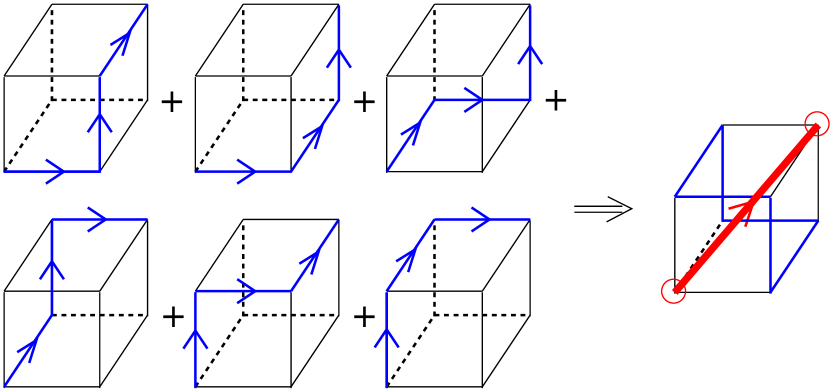
Figure 1: $b=\sqrt{3}$ blocking transformation.

The parameter $\kappa$ is tuned to optimize the locality of the FP action. Expanding the FP action to quadratic order in the gluon fields gives

$$\frac{1}{V^{(1)}}\sum_{k^{(1)}}\rho^{(1)}_{mn}(k^{(1)}){\rm Tr}[B_{m}^{*}(k^{(1)})B_{n}(k^{(1)})]=$$

$$\min_{A}\bigg{(}\frac{1}{V^{(0)}}\sum_{k^{(0)}}\rho^{(0)}_{\mu\nu}{\rm Tr}[A_{\mu}^{*}(k^{(0)})A_{\nu}(k^{(0)})]+$$

$$\frac{\kappa}{V^{(1)}}\sum_{k^{(1)}}{\rm Tr}\mid\Gamma_{m}(k^{(1)})-B_{m}(k^{(1)}))\mid^{2}\bigg{)}$$ (24)

$B_{m}$ and $A_{\mu}$ are gluon fields on the coarse and fine lattice respectively, $k^{(0)}=(k^{(1)}/\sqrt{3})+h^{(1)}$, $V^{(0)}=9V^{(1)}$. We use Greek indices for periodic lattice and Roman indices for the twisted lattice. Lastly,

$$\Gamma_{m}(k^{(1)}) \equiv \frac{1}{9}\sum_{h^{(1)}}\omega^{(1)}_{m\nu}(k^{(0)})A_{\nu}(k^{(0)})$$ (25)

$$\omega^{(1)}_{x1}(k) = \frac{1}{4}\bigg{(}\frac{2\hat{k}_{2}}{\hat{k}_{2}}\bigg{)}\bigg{(}\frac{2\hat{k}_{3}}{\hat{k}_{3}}\bigg{)}+\frac{1}{12}\hat{k}_{2}\hat{k}_{3}$$ (26)

and similar expressions for the other components of $\omega^{(1)}$. The matrices $\omega^{(1)}$ and vectors $h^{(1)}$ contain all the details of the RGT. Solving Eq. (24) leads to the recursion relation for $D^{(i)}\equiv(\rho^{(i)})^{-1}$:

$$D^{(1)}_{ml}(k^{(1)})=$$

$$\frac{1}{9}\sum_{h^{(1)}}\omega^{(1)}_{m\mu}(k^{(0)})D^{(0)}_{\mu\beta}(k^{(0)})\omega^{(1)}_{\beta l}{}^{\dagger}(k^{(0)})+\delta_{ml}\frac{1}{\kappa}$$ (27)

Similarly, the recursion relation for $T_{2}$ is obtained by changing $(0)\rightarrow(1)$, $(1)\rightarrow(2)$, and $\mu({\rm Greek})\leftrightarrow m({\rm Roman})$.

$$\omega^{(2)}_{1x}(k) = \frac{1}{4}\bigg{(}\frac{2\hat{k}_{y}}{\hat{k}_{y}}\bigg{)}^{*}\bigg{(}\frac{2\hat{k}_{z}}{\hat{k}_{z}}\bigg{)}+\frac{1}{12}\hat{k}_{y}^{*}\hat{k}_{z}$$ (28)

The specific choice of $T_{1}$ given in Eq. (13) is not unique. There are eight equivalent independent choices. So for each $T_{2}\otimes T_{1}$, we average over the eight to regain hypercubic invariance.

2 Numerical study of FP action

To find the FP we start with $D^{(0)}$ equal to the free propagator in Feynman gauge and numerically iterate the recursion relations Eqs. (27) until $D^{(2n)}$ satisfies the fixed-point requirement: for a given precision criterion $\epsilon$ and $\forall k$ in the $(2n)$-th Brillion zone,

$$\mid D^{(2n)}_{\mu\nu}(k)-D^{(2n-2)}_{\mu\nu}(k)\mid<\epsilon.$$ (29)

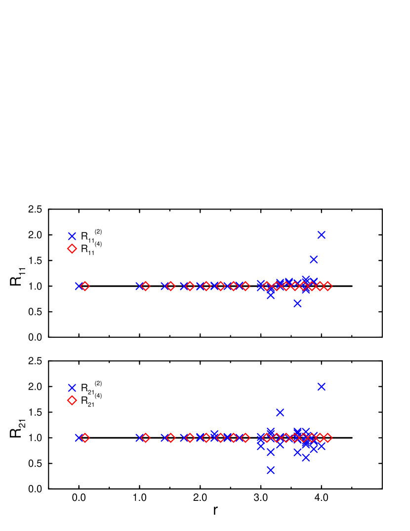
Figure 2: Finite volume effect.

We now discuss results. First, in Fig. 2, we show the ratios:

$$R_{\mu\nu}^{(2)}=\frac{\rho_{\mu\nu}(L:24\rightarrow 8)}{\rho_{\mu\nu}(L:216\rightarrow 72)}$$

$$R_{\mu\nu}^{(4)}=\frac{\rho_{\mu\nu}(L:72\rightarrow 24)}{\rho_{\mu\nu}(L:216\rightarrow 72)}$$

to show finite volume corrections. On the $8^{4}$ lattice, we observe $\ll 1\%$ deviation for $r\equiv|x|\leq 2$, which grow significantly for $r\gtrsim 3$. Since no correction is observed on the $24^{4}$ lattice, we assume that $\rho(L:216\rightarrow 72)$ gives infinite volume results in the range $r\lesssim 4$, and $24^{4}$ coarse lattice is sufficient for the calculation.

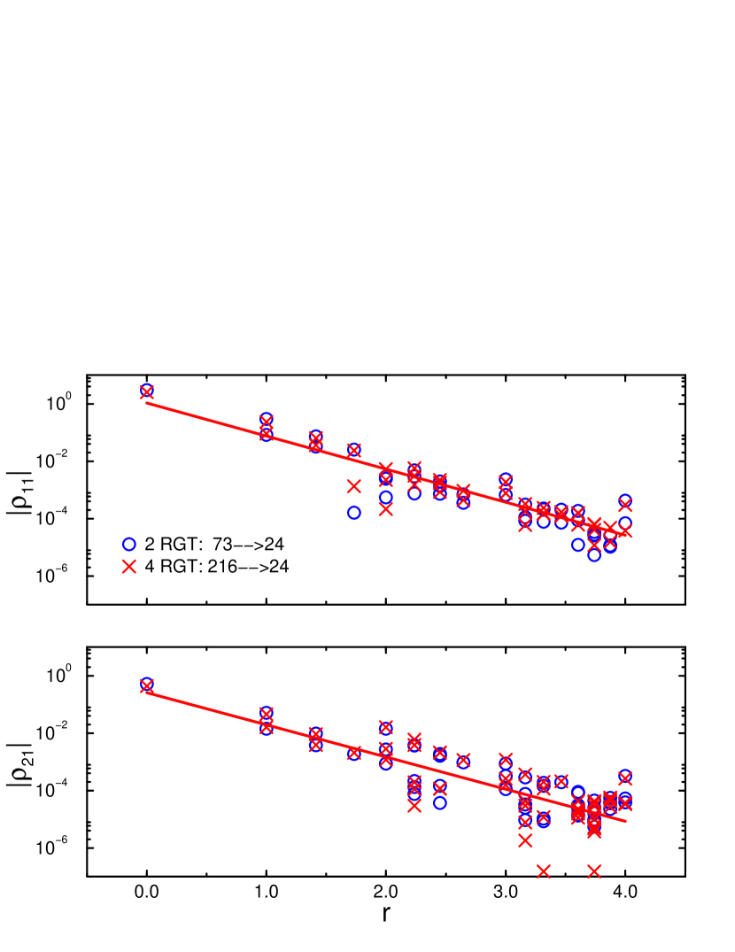
Figure 3: Minimal $\chi^{2}$ fitting at $\kappa=12.0$.

Second, we optimize $\kappa$ for maximal locality in both in $\rho_{11}$ and $\rho_{21}$ couplings. We define the locality parameter $\xi$ as

$$\mid\rho_{\mu\nu}(r)\mid=Z\exp\left(-\frac{r}{\xi_{\mu\nu}}\right)$$ (30)

Fig. 3 shows a least square fit which determines $\xi$. Since the fit is very sensitive to $r\geq 2$, we only use the $24^{4}$ lattice results obtained by 4 RGT iterations to avoid finite volume effects. The maximal locality is found at $\kappa=39.5$ for $\xi_{11}$ and $\kappa=29.5$ for $\xi_{21}$ as shown in Fig. 4.

$\rho_{00}(r)$			$\rho_{10}(r)$
r	$b=\sqrt{3}$	$b=2$ (I)	r	$b=\sqrt{3}$	$b=2$ (I)
0001	$-0.4110$	$-0.6718$	0000	$-0.6977$	$-0.8007$
1000	$-0.2909$	$-0.0595$	0001	$-0.0686$	$-0.0310$
0011	$-0.1027$	$-0.0428$	0100	$+0.0524$	$+0.0113$
1001	$+0.0645$	$+0.0161$	0101	$-0.0019$	$-0.0021$
0111	$-0.0336$	$-0.0272$	1011	$+0.0126$	$+0.0088$
1011	$+0.0053$	$-0.0027$	2100	$+0.0109$	$-0.0039$
1111	$-0.0020$	$-0.0037$	0111	$-0.0020$	$-0.0010$
0002	$+0.0145$	$+0.0242$	0002	$+0.0766$	$-0.0017$

Table 1: $\rho_{\mu\nu}(r)$ after 6 iterations of $b=\sqrt{3}$ RGT.

Our optimal choice is taken to be $\kappa=27.5$ and we present the corresponding $\rho_{\mu\nu}$ in Tab. 1. For comparison we also give the results for $b=2$ RGT first obtained in [2]. We are not able to comment on which RGT is “better” due to the issue of redundant operators; numerical tests of scaling need to be done.

Finally, the results for the couplings given in Tab. 1 are expressed in terms of coefficients of Wilson loops in Tab. 2. Simulations to check the efficacy of this action need to be done.

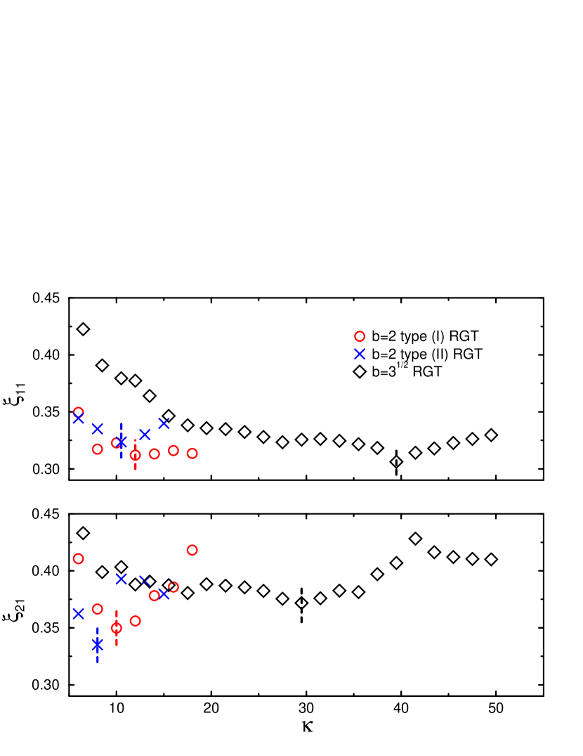
Figure 4: $\xi_{\mu\nu}$ with repect to $\kappa$.

Wilson Loop	coefficients
(x,y,-x,-y)	$+0.6285$
(x,y,y,-x,-y,-y)	$-0.0830$
(x,y,z,-x,-y,-z)	$+0.0419$
(x,y,x,z,-x,-y,-x,-z)	$-0.0041$
(x,y,y,-x,z,-y,-y,-z)	$+0.0060$
(x,y,y,-x,-x,-y,-y,x)	$+0.0105$
(x,y,z,t,-x,-y,-z,-t)	$+0.0062$

Table 2: Coefficients of Wilson loops in the FP action.

References

[1] R. Cordery, R. Gupta, M. Novotny, Phys. Lett. B128
(1983) 425.