?abstractname?

The static potential in the confinement “phase” of the SU(2) Higgs model is studied. In particular, the observation of the screening (called string breaking) of the static quarks by the dynamical light quarks leading to the formation of two static-light mesons was not observed before my work in non-Abelian gauge theories. The tool that I employ is lattice gauge simulation. The observable from which the spectrum of the Hamiltonian in presence of two static quarks can be extracted, is a matrix correlation whose elements are constructed not only from string-type states represented by Wilson loops (like in pure gauge theories). Additional matrix elements representing transitions from string-type to meson-type states and the propagation of meson-type states are taken into account. From this basis of states it is possible to extract the ground state and first excited state static potentials employing a variational method. The crossing of these two energy levels in the string breaking region is clearly visible and the inadequacy of the Wilson loops alone can be demonstrated. I also address the question of the lattice artifacts. For this purpose lines of constant physics in the confinement “phase” of the model have to be constructed. This problem has only partially been solved. Nevertheless it is possible to show that the static potentials have remarkable scaling properties under a variation of the lattice spacing by a factor two and are almost independent of the quartic Higgs coupling.

?contentsname?

1. 1 Introduction
2. 2 The SU(2) Higgs model
   1. 2.1 Definition of the model
   2. 2.2 Symmetries
   3. 2.3 Phase diagram
   4. 2.4 Monte Carlo simulation
   5. 2.5 Statistical error analysis
      1. 2.5.1 Primary quantities
      2. 2.5.2 Binning
      3. 2.5.3 Secondary quantities: jackknife binning
3. 3 Static-light mesons
   1. 3.1 Variational method
   2. 3.2 One-link integral
   3. 3.3 Meson-type operators
4. 4 String breaking
   1. 4.1 Matrix correlation
   2. 4.2 Results at $\beta=2.4$
      1. 4.2.1 Static potential $\mathbf{V_{0}}$
      2. 4.2.2 Scale $\mathbf{r_{0}}$
      3. 4.2.3 Renormalised static potentials $\mathbf{r_{0}\,[V(r)-2\mu]}$
      4. 4.2.4 Overlaps
      5. 4.2.5 Level crossing
5. 5 Scaling
   1. 5.1 Matching of $\kappa$
   2. 5.2 Matching of $\lambda$
      1. 5.2.1 Cumulants
      2. 5.2.2 Higgs and W-boson correlations
   3. 5.3 Scaling
      1. 5.3.1 Cumulants
      2. 5.3.2 Higgs and W-boson correlations
      3. 5.3.3 Static potentials
6. 6 Conclusions and Outlook
7. A Notation conventions
   1. A.1 Lattice notation
   2. A.2 SU($N$) gauge fields
   3. A.3 SU(2) Higgs field
8. B The transfer matrix in the SU(2) Higgs model
   1. B.1 Hamiltonian formalism
   2. B.2 The transfer matrix in the temporal gauge
      1. B.2.1 Positivity
   3. B.3 Charge sectors
      1. B.3.1 Minkowski space continuum
      2. B.3.2 Lattice formulation
   4. B.4 Reconstruction of the Euclidean expectation values
      1. B.4.1 Reconstruction theorem
      2. B.4.2 The static potential
9. C Updating algorithms
   1. C.1 Random Numbers
   2. C.2 Updating of the gauge field
      1. C.2.1 Heatbath
      2. C.2.2 Overrelaxation
   3. C.3 Updating of the Higgs field
      1. C.3.1 Heatbath
      2. C.3.2 Overrelaxation
10. D One-link integral and approximation of the modified Bessel functions
11. E Parallelisation
    1. E.1 Geometry of the two-dimensional partition
    2. E.2 Communication between PEs
    3. E.3 Program overview

?chaptername? 1 Introduction

The success of the quark-constituent picture both for resonances and for deep-inelastic electron and neutrino processes makes it difficult to believe quarks do not exist. The problem is that quarks have not been seen.
K.G. Wilson, 1974

The theory of strong interactions plays a pivotal role in particle physics. It is part of the Standard Model of elementary particles which successfully describes the constituents of the matter in terms of quantum gauge field theories. These theories are based on the gauge principle [1]: the fields in the theory have internal degrees of freedom associated with a gauge group and it is required that local transformations of these degrees of freedom leave the physics unchanged. The gauge group of the Standard Model is ${\rm SU(3)}_{c}\times{\rm SU(2)}_{\rm L}\times{\rm U(1)}_{\rm Y}$ and the degrees of freedom associated with them are color for SU(3), weak (left-handed) isospin for SU(2) and hypercharge for U(1). The gauge group together with the gauge principle dictate the structure and properties of the interactions. The particle content, described by means of relativistic local quantum fields, has to be deduced from what nature tells us.

The particles which take part in strong interactions are called hadrons: Gell-Mann and Zweig [2, 3] proposed a model that explained the low energy properties of the hadrons (like mass and spin) in terms of elementary constituents called quarks. Bjorken [4] studied, within the framework of current algebra, the electron-nucleon scattering and discovered the scaling property of the structure functions for large electron momentum transfer (deep inelastic scattering). The Bjorken scaling was experimentally confirmed and could be understood with the assumption that the electrons scatter off almost-free pointlike constituents [5] inside the nucleon, which were called partons [6, 7]. Later the partons were identified with the quarks on the basis of their quantum numbers. The question at that moment was to find a theory in which particles are free at high energies. The decisive step was then made with the proof that non-Abelian gauge field theories exhibit asymptotic freedom [8, 9, 10]. The strength of the interaction given by the gauge coupling becomes weak at shorter distances (or equivalently at high energies) and this is consistent with the Bjorken scaling. In order to resolve several difficulties of the quark model, like the construction of an antisymmetric wave function for the $\Delta^{++}$ baryon and the discrepancy between the prediction and experimental data on the total cross section $e^{+}e^{-}\to\mbox{hadrons}$, it was already suggested that quarks must have a new quantum number called color and exhibit color symmetry. Fritzsch, Gell-Mann and Leutwyler [11] proposed that the theory describing the quark dynamics is a non-Abelian gauge theory with gauge group SU(3) associated with the color symmetry. This theory was named quantum chromodynamics (QCD): its ingredients are quarks and gluons, usually called partons. The gluons are the vector bosons that mediate the interactions: in contrast with an Abelian gauge field theory where the vector boson (the photon) is gauge neutral, the gluons carry color quantum numbers and therefore have self-interactions. It is this property which is responsible for asymptotic freedom. Due to asymptotic freedom, the short distance behavior of the partons can be described with a perturbative expansion in the small value of the gauge coupling. Within the perturbative approach, QCD found important confirmations as the theory of strong interactions, such as the prediction of a logarithmic deviation from Bjorken scaling in structure functions, confirmed experimentally in deep inelastic lepton-nucleon scatterings.

What is observed in nature are not the partons, but the hadrons, which are color-neutral objects. The fact that colored partons cannot be seen isolated led to the conjecture of color confinement: the partons are always bound into the hadrons. In order to prove this assumption from QCD one should be able to describe its properties at long distances corresponding to the size of the hadrons. Perturbation theory is not applicable because the gauge coupling is large at this scale. Wilson [12] proposed in 1974 a new approach to gauge field theories amounting to the discretisation of the four-dimensional space-time on a Euclidean lattice. The quantisation of this theory is naturally performed in the path integral formalism. The matter fields are treated as classical variables living on the points of the lattice and the gauge field is represented by connections (links) between the matter fields on nearest-neighbor points. The quantum effects in the observables of the theory are introduced by evaluating their expectation values expressed as Feynman path integrals [13]. In the Euclidean lattice formulation, a quantum field theory looks like a classical statistical system. Particle and solid state physics mutually profited by this relationship [14]. The concept of renormalisation of a gauge field theory receives new insights. The regularisation of the theory on the lattice is associated with an ultraviolet cut-off, the inverse lattice spacing $a^{-1}$. The field theory is changed in the short distance region while its long distance properties are preserved. The question one is interested in, is whether there is the possibility of constructing a continuum quantum field theory from the lattice field theory: that is, is the limit $a\to 0$ of the lattice field theories well defined? To answer this question, we should be able to reproduce the same physical situation on lattices with different cut-offs $a$ and consider the behavior of dimensionless physical quantities when $a\to 0$. The equations describing the change in the parameters of the theory under variation of the lattice spacing $a$ are the renormalisation group equations (RGEs) of the lattice field theory. One consequence of the RGEs is that the continuum limit of a lattice regularised asymptotically-free theory is reached when the lattice bare gauge coupling $g$ is sent to zero. To show the correspondence between a lattice field theory and a statistical system one considers the field propagator on the lattice. For example, in a statistical system of Ising spins, the corresponding quantity is the spin-spin correlation, whose exponential decay is governed by the correlation length. On the lattice, the correlation length equals the inverse mass gap. By keeping the mass gap fixed at its physical value, the correlation length expressed in units of $a$ diverges in the continuum limit. Thus, the continuum limit of a lattice field theory, if it exists, corresponds to a second order phase transition in the parameter space of the statistical system.

?figurename? 1.1: The Wilson loop, here represented on a lattice, describes the confinement of static quarks.

Wilson [12] originally proposed lattice gauge theories in order to explain color confinement. To this end, he derived an expansion valid for strong gauge coupling in which confinement arises naturally. However, in non-Abelian gauge theories the continuum limit is reached when $g\to 0$ due to asymptotic freedom. Another method must be developed to study the confinement in the weak gauge coupling regime. We consider the system composed of a pair of infinitely heavy or static quark and anti-quark. The static quark (anti-quark) is treated as an external source in the (complex conjugate of the) fundamental representation of the gauge group. In pure SU($N$) Yang-Mills gauge theories, the potential between the static quarks, called the static potential, can be extracted in the path integral formalism from the expectation value of Wilson loops represented in Fig. 1.1. On the lattice, they are defined as the trace of the product of the gauge links $U$ over a closed path composed of two straight time-like lines and arbitrary space-like paths C and ${\rm C}^{\prime}$ connecting the time-like lines:

$$\langle W_{{\rm C}{\rm C^{\prime}}}\rangle\;=\;\langle\,\hbox{tr}\,\prod U\rangle {}_{\mbox{$\stackrel{{\scriptstyle\displaystyle\sim}}{{\scriptstyle t\to\infty}}$}} {\rm e}^{-t\cdot V_{\rm Q\bar{\rm Q}}(\vec{x}-\vec{y})}\,,$$ (1.1)

where $t$ is the time extension of the Wilson loop and $V_{\rm Q\bar{\rm Q}}(r)$ is the static potential for the separation $r$ of the static quarks. The expectation value in eq. (1.1) can be computed by Monte Carlo simulation of the Yang-Mills theory on the lattice. The seminal work was done by Creutz [15] for the gauge group SU(2) and since then, there have been a number of detailed studies which show a linear confinement potential at large distances between the static quarks close to the continuum limit, both for gauge group SU(2) [16, 17] and SU(3) [18, 19].

When the Yang-Mills gauge theories are coupled to matter fields in the fundamental (quark) representation of the gauge group, the potential between a pair of static quarks is expected to flatten at large distances: the ground state of the system is better interpreted in terms of two weakly interacting static-light mesons which are bound states of a static and a dynamical quark. The dynamical quarks are pair-created in the strong gauge field binding the static quarks. This phenomenon is called string breaking or screening of the static charges. The name “string” refers to the gauge field configuration which confines the static quarks and leads to the linear confinement in pure gauge theories.

In recent attempts in QCD with two flavors of dynamical quarks, this string breaking effect was not visible [20, 21, 22, 23, 24, 25]. The string breaking distance $r_{\rm b}$ around which the static potential should start flattening off, could nevertheless be estimated in the so called quenched approximation of QCD to be [26]

$$r_{\rm b} \approx 2.7r_{0}\,,$$ (1.2)

where the scale $r_{0}\approx 0.5\,{\rm fm}$ was introduced in [17]. The static potential at short distances and the mass of the static-light meson can be computed in quenched QCD. The approximate value in eq. (1.2) was obtained from the crossing point of the linearly rising potential with twice the value of the meson mass (which is expected to be the asymptotic value of the potential after string breaking).

The investigation of the static potential in models other than QCD is therefore relevant in order to understand its origin and identify possible failures of the methods used to extract it. First studies of string breaking were performed with a hopping-parameter expansion in SU(2) gauge theory with Wilson fermions [27]. In the Schwinger model, which is quantum electrodynamics (QED) in two dimensions, the exact solution for the static potential can be given in the limit of zero fermion mass [28]: $V(r)=(e\sqrt{\pi}/2)\{1-\exp(-er/\sqrt{\pi})\}$, where $e$ is the charge of the static sources. String breaking was established by numerical simulation in the Schwinger model [29, 30]. Numerical evidence of the screening of the static potential was also found in the U(1) Higgs model (scalar QED) in two dimensions [31]. The flattening of the static potential at large distances is also expected in the confinement “phase” of the SU(2) Higgs model. Indeed, early simulations yielded some qualitative evidence for string breaking [32, 33].

String breaking can also be studied in Yang-Mills theories using static sources in the adjoint representation of the gauge group. The gauge field itself is responsible for the screening of the sources and the formation of hadrons called “gluelumps”. An important numerical investigation concerning this screening has been carried out by C. Michael in [34], where it has been noted that string breaking can be a mixing phenomenon. The static potential is extracted from a matrix correlation in which two types of states enter, the adjoint “string” and the “two-gluelump”. However, due to large errors, no clear evidence for string breaking could be given. The first numerical evidence using the mixing method for string breaking in non-Abelian gauge theories with dynamical matter fields, was given in the four-dimensional [35] and three-dimensional [36] SU(2) Higgs model by the computation of the potential between static quarks. Most recently, the extraction of the static adjoint potential in the three-dimensional SU(2) Yang-Mills theory [37, 38] shows also evidence for string breaking.

Finally, we want to mention that string breaking has been seen in finite temperature QCD [39], where the static potential can be extracted from Polyakov loop correlators.

The status quo before our work, was that no clear evidence for string breaking in non-Abelian gauge theories was established. In our research, we investigate the potential between static quarks in the four dimensional SU(2) Higgs model on the lattice. In Chapt. 2, we describe the model. The parameter space of the theory is divided in two “phases”, the confinement and the Higgs “phase”. In the confinement “phase”, the properties are similar to QCD: screening of external charges by the dynamical Higgs field is expected. We describe the error analysis of the statistical measurements.

In Chapt. 3, we concentrate on the determination of the mass spectrum of the static-light mesons, which are expected to be the asymptotic states after string breaking. We describe the variational method that we use for extracting the energy spectrum from a matrix correlation function constructed with a basis of states that can mix. We will use the same method for the determination of the static potential. The basis of states is enlarged by the use of smeared fields: we present a study of different smearing procedures for the Higgs field.

In Chapt. 4, we introduce the matrix correlation function from which we extract the static potential. We use two “types” of states: “string states” and “two-meson states”. The variational method determines the best linear combination approximating the true eigenstates of the Hamiltonian. We present the results for $\beta=4/g^{2}=2.4$, where $g$ is the gauge coupling. We are able to determine the ground state and first excited state static potential with good accuracy. This allows us to study the overlaps of the approximate eigenstates, determined from our basis of states, with the true eigenstates. For comparison with the recent studies of string breaking in QCD, we analyse what happens if we use only the Wilson loops for determining the ground state static potential.

In Chapt. 5, we address the question of the “continuum limit”: in order to investigate lattice artifacts in our results, we would like to reproduce the physical situation of Chapt. 4 on a coarser lattice at $\beta=2.2$. In the parameter space of the model, this would define a line of constant physics (LCP), along which two dimensionless physical quantities are kept constant under variation of the lattice spacing. The static potential provides us with a first quantity sensitive to the mass of the dynamical Higgs field. We study the definition of a second quantity sensitive to the quartic Higgs coupling. Although we are not able to match precisely the parameters along the LCP, we find a parameter region in which the discussion of the scaling properties of different quantities, in particular the static potentials, is possible.

In Chapt. 6, we summarise the results of our work and give some prospectives for future investigations.

A number of more technical information is relegated to appendices. In Appendix A, we explain the notation conventions that we use throughout the work. In Appendix B, we construct the transfer matrix operator for the SU(2) Higgs model and prove its positivity, which is the condition for a real energy spectrum of the theory. The connection between path integral expectation values and vacuum expectation values of corresponding time ordered operators is also shown. In Appendix C, we describe our algorithms for the Monte Carlo simulation of the SU(2) Higgs model. In Appendix D, we explain the implementation of the one-link integral method which allows the reduction of the statistical variance of the correlation functions. Finally, Appendix E is devoted to the description of the parallelised computer program that we use for the Monte Carlo simulations.

?chaptername? 2 The SU(2) Higgs model

2.1 Definition of the model

The SU(2) Higgs model on a four-dimensional Euclidean lattice is defined by means of a gauge field of dimensionless SU(2) matrices $U(x,\mu)$ and a complex Higgs field $\Phi(x)$ in the fundamental representation of the gauge group SU(2) and with canonical mass dimension one. The full action is

$$S=S_{{\rm W}}+\sum_{x}a^{4}\bigg{\{}\sum_{\mu}\left(\nabla_{\mu}\Phi(x)\right)^{\dagger}\left(\nabla_{\mu}\Phi(x)\right)$$

$$\qquad+\;m_{0}^{2}\Phi^{\dagger}(x)\Phi(x)+\lambda_{0}\left[\Phi^{\dagger}(x)\Phi(x)\right]^{2}\bigg{\}}\,,$$ (2.1)

where $S_{{\rm W}}$ is the Wilson action eq. (A.8) for the SU(2) gauge field. Introducing the dimensionless lattice fields $\Phi_{{\rm L}}=(a/\sqrt{\kappa})\Phi$ (we drop the subscript L in the following) together with the new couplings $\lambda=\kappa^{2}\lambda_{0}$ and $\kappa=(1-2\lambda)/(8+a^{2}m_{0}^{2})$ the action can be written as

$$S=S_{{\rm W}}+\sum_{x}\bigg{\{}\Phi^{\dagger}(x)\Phi(x)+\lambda\left[\Phi^{\dagger}(x)\Phi(x)-1\right]^{2}$$

$$-\kappa\sum_{\mu}\left[\Phi^{\dagger}(x)U(x,\mu)\Phi(x+a\hat{\mu})+\Phi^{\dagger}(x+a\hat{\mu})U^{\dagger}(x,\mu)\Phi(x)\right]\bigg{\}}\,.$$ (2.2)

The physics of the model is controlled by the three dimensionless bare parameters $\beta\equiv 4/g^{2},\;\kappa,\;\lambda$. We will use the parametrisation eq. (2.1) throughout the work. We can rewrite eq. (2.1) using the $2\times 2$ matrix notation for the Higgs field $\varphi(x)=\rho(x)\alpha(x),\;\rho(x)\geq 0,\;\alpha(x)\in{\rm SU(2)}$ defined in Sect. A.3:

$$S=S_{{\rm W}}+\sum_{x}\bigg{\{}\frac{1}{2}\,\hbox{tr}\,(\varphi^{\dagger}(x)\varphi(x))+\lambda\left[\frac{1}{2}\,\hbox{tr}\,(\varphi^{\dagger}(x)\varphi(x))-1\right]^{2}$$

$$\qquad-\kappa\sum_{\mu}\,\hbox{tr}\,(\varphi^{\dagger}(x)U(x,\mu)\varphi(x+a\hat{\mu}))\bigg{\}}\,.$$ (2.3)

The gauge and Higgs field are both represented as $2\times 2$ matrices which are equal to a real constant times an SU(2) matrix. This is particularly useful for programming purposes, see Sect. E.2.

The Euclidean expectation value of an observable $O[U,\Phi]$ is defined by the Feynman path integral

$$\langle O\rangle = \frac{1}{Z}\int{\rm D}[U]\,{\rm D}[\phi]\,O[U,\Phi]\,{\rm e}^{-S[U,\Phi]}\,,$$ (2.4)

where $Z$ is the partition function

$$Z = \int{\rm D}[U]\,{\rm D}[\phi]\,{\rm e}^{-S[U,\Phi]}\,,$$ (2.5)

${\rm D}[U]$ denotes the product measure $\prod\limits_{x,\mu}{\rm d}U(x,\mu)$ (${\rm d}U$ is the Haar measure on SU(2)) and ${\rm D}[\phi]$ denotes $\prod\limits_{x}{\rm d}\phi_{1}(x)\cdot\cdot\cdot{\rm d}\phi_{4}(x)$. The fields $\phi_{i}(x)\;(i=1,2,3,4)$ are the four real components of $\Phi(x)$ defined in eq. (A.16).

The expectation values in eq. (2.4) can be shown to correspond to Euclidean vacuum expectation values of corresponding time-ordered operators for large enough time extent of the lattice. This correspondence can be established through the definition of a time evolution operator called transfer matrix. How this is done for the SU(2) Higgs model is the subject of Appendix B.

The lattice formulation of a quantum field theory provides a mathematically well-defined, non-perturbative and completely finite regularisation of the theory. An analytical solution of eq. (2.4) is in the most cases not possible, but it can be computed with Monte Carlo algorithms. The overall aim [40] is to generate a representative ensemble of field configurations $\{[U_{n},\Phi_{n}],\;n=1,2,...,N\}$ for the path integral eq. (2.4) by employing a stochastic process. Representative means that the probability distribution of the configurations in the ensemble is the Boltzmann distribution $\exp(-S[U,\Phi])$. We evaluate then eq. (2.4) as the ensemble average

$$\overline{O} = \frac{1}{N}\sum_{i=1}^{N}O[U_{n},\Phi_{n}]\,.$$ (2.6)

The value $\overline{O}$ has a statistical error $\Delta(O)$. Moreover, in most cases one is interested in secondary quantities, which are functions of the primary averages $\overline{O}$.

The methods that we use for the Monte Carlo simulation of the model are described in detail in Appendix C. The determination of the statistical errors will be the subject of Sect. 2.5.

2.2 Symmetries

We dedicate a section to the discussion of symmetries of the action and integration measure which reflect themselves in useful properties of the expectation values defined by eq. (2.4).

Let us start from the four-component $\phi^{4}$ theory without gauge interactions. The four components of the scalar field $\phi_{i}(x)\;(i=1,2,3,4)$ can be put in a $2\times 2$ matrix as described in Sect. A.3. In this notation the action of the pure scalar theory is

$$S_{\phi}=\sum_{x}\bigg{\{}\frac{1}{2}\,\hbox{tr}\,(\varphi^{\dagger}(x)\varphi(x))+\lambda\left[\frac{1}{2}\,\hbox{tr}\,(\varphi^{\dagger}(x)\varphi(x))-1\right]^{2}$$

$$\qquad-\kappa\sum_{\mu}\,\hbox{tr}\,(\varphi^{\dagger}(x)\varphi(x+a\hat{\mu}))\bigg{\}}\,.$$ (2.7)

The model is symmetric under the global O(4) transformation $\phi^{\prime}_{i}(x)=R_{ij}\phi_{j}(x)$, where $R\in{\rm O}(4)$. In the matrix notation for the scalar field this transformation is equivalent to a global ${\rm SU(2)}_{{\rm L}}\otimes{\rm SU(2)}_{{\rm R}}$ symmetry defined as

$$\varphi(x) \longrightarrow A_{{\rm L}}^{\dagger}\varphi(x)A_{{\rm R}}\quad,\quad A_{{\rm L,R}}\in{\rm SU(2)}\,.$$ (2.8)

The SU(2) Higgs model is obtained by gauging the subgroup ${\rm SU(2)}_{{\rm L}}$, i.e. by “promoting” the global symmetry associated with the group ${\rm SU(2)}_{{\rm L}}$ to a local symmetry. According to the gauge principle [1], this automatically requires the appearance of the gauge field $U(x,\mu)$ and of interactions. We end up precisely with the action in eq. (2.1). Under gauge transformation defined by the field of SU(2) matrices $\{\Lambda(x)\equiv A_{{\rm L}}(x)\}$ the fields transform as

$$U^{\Lambda}(x,\mu) = \Lambda^{\dagger}(x)U(x,\mu)\Lambda(x+a\hat{\mu})$$ (2.9)

$$\varphi^{\Lambda}(x) = \Lambda^{\dagger}(x)\varphi(x)\,.$$ (2.10)

The SU(2) Higgs model has a residual global SU(2) symmetry defined by the diagonal subgroup $A_{{\rm L}}=A_{{\rm R}}=A$:

$$\varphi(x) \longrightarrow A^{\dagger}\varphi(x)A\,,$$ (2.11)

$$U(x,\mu) \longrightarrow A^{\dagger}U(x,\mu)A\,.$$ (2.12)

This symmetry is called the (weak) isospin.

Let us now discuss the symmetry under gauge transformation. The action of the SU(2) Higgs model eq. (2.1) is invariant under the gauge transformations eq. (2.9) and eq. (2.10) per construction. The integration measure in eq. (2.4) as well: for the gauge field the property ${\rm d}U={\rm d}U^{\Lambda}$ is a consequence of the invariance of the Haar measure: ${\rm d}U={\rm d}(UV)={\rm d}(VU)$ for $V\in SU(2)$. For the Higgs field we note that

$$\int_{\mathchoice{\rm I\kern-1.47005pt{R}}{\rm I\kern-1.47005pt{R}}{\rm I\kern-1.33002pt{R}}{\rm I\kern-1.33002pt{R}}^{4}}{\rm d}\phi_{1}(x)\cdot\cdot\cdot{\rm d}\phi_{4}(x) \propto \int_{0}^{\infty}\rho^{3}{\rm d}\rho\int_{{\rm SU(2)}}{\rm d}\alpha\,,$$ (2.13)

if we write the Higgs field in the notation of eq. (A.19) $\varphi(x)=\rho(x)\alpha(x)$. From $\varphi^{\Lambda}(x)=\rho(x)(\Lambda^{\dagger}(x)\alpha(x))$ the invariance of the measure follows immediately. Defining $O^{\Lambda}[U,\Phi]=O[U^{\Lambda},\Phi^{\Lambda}]$ as the gauge transform of the observable $O$, we therefore have the property

$$\langle O^{\Lambda}\rangle = \langle O\rangle\,.$$ (2.14)

In the continuum SU(2) Higgs model one speaks of Higgs and W-boson fields which are not gauge invariant: a particular gauge is fixed and perturbation theory can then be applied. In the non-perturbative lattice scheme one does not need to fix the gauge and gauge-invariant definitions of interpolating fields for the Higgs and W-bosons have then to be used. A gauge invariant composite Higgs field is defined as

$$H(x) = \Phi^{\dagger}(x)\Phi(x)\;=\;\frac{1}{2}\,\hbox{tr}\,(\varphi^{\dagger}(x)\varphi(x))\,.$$ (2.15)

It is an isospin 0 scalar field. A gauge invariant W-boson field is defined as

$$W_{r\mu}(x) = -i\,\hbox{tr}\,(\tau_{r}V_{\mu}(x))\quad(r=1,2,3)\,,$$ (2.16)

$$V_{\mu}(x) = \alpha^{\dagger}(x)U(x,\mu)\alpha(x+a\hat{\mu})\,,$$ (2.17)

where $V_{\mu}(x)$ is called the gauge invariant link variable. The field in eq. (2.16) is an isospin 1 (with isospin index $r$) spin 1 vector field. The isospin property can be seen transforming the field under the isospin transformations eq. (2.11) and eq. (2.12) and using the relation

$$A\tau_{r}A^{\dagger} = R(A)_{sr}\tau_{s}\,,\quad A\in{\rm SU(2)},\;R(A)\in{\rm SO(3)}\,,$$ (2.18)

which defines $R(A)$ as the adjoint (isospin=1) representation of the isospin group SU(2).

Another symmetry of the action and the integration measure is under complex conjugation of the field variables, $U_{ab}(x)\rightarrow U_{ab}^{*}(x),\;\Phi_{a}(x)\rightarrow\Phi_{a}^{*}(x)$. For the measure this symmetry is a consequence of the equivalence of the representation 2 and $2^{*}$ of SU(2) eq. (A.13). For an observable of the form $L=\Phi^{\dagger}(x)U(x,y)\Phi(y)$, where $U(x,y)$ is a link path connecting $y$ with $x$, we can write $L^{*}=(\Phi^{*}(x))^{\dagger}U^{*}(x,y)\Phi^{*}(y)$ from which it follows

$$\langle L^{*}\rangle = \langle L\rangle\,.$$ (2.19)

The reality of the action and the measure gives the result $\langle L\rangle\in\mathchoice{\rm I\kern-2.10007pt{R}}{\rm I\kern-2.10007pt{R}}{\rm I\kern-1.90002pt{R}}{\rm I\kern-1.90002pt{R}}$.

2.3 Phase diagram

The bare parameters $\kappa,\;\lambda$ are restricted to the ranges $\kappa\geq 0,\;\lambda\geq 0$. A negative value of $\lambda$ would lead to an action which is not bounded from below and therefore the path integral eq. (2.4) would not be well defined. With the help of the transformation

$$\Phi(x) \longrightarrow \left\{\begin{array}[]{ll}-\Phi(x)&\mbox{if}\quad(-1)^{\sum_{\mu}x_{\mu}/a}=1\\ \Phi(x)&\mbox{if}\quad(-1)^{\sum_{\mu}x_{\mu}/a}=-1\end{array}\right.$$ (2.22)

it is easy to see that the partition function eq. (2.5) has the following symmetry

$$Z(\beta,\kappa,\lambda) = Z(\beta,-\kappa,\lambda)\,.$$ (2.23)

Replacing $\kappa$ with $-\kappa$ corresponds merely to a change in the description of the model and leaves the physics of the model invariant: with the help of the transformation eq. (2.22) we can define a mapping of the observables of the model such that the expectation values eq. (2.4) computed with parameter $\kappa$ are reproduced by expectation values computed with parameter $-\kappa$. Without loss of generality we can therefore restrict ourselves to the parameter range $\kappa\geq 0$.

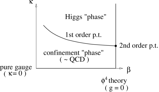
?figurename? 2.1: The phase diagram of the SU(2) Higgs model in the $(\beta,\kappa)$ plane is shown for a typical value of $\lambda$.

Fig. 2.1 shows the phase structure of the SU(2) Higgs model [40, 41]. In the $(\beta,\kappa)$ plane there is a line which is believed to be a first order phase transition line separating the confinement “phase” at small values of $\kappa$ from the Higgs “phase” at larger $\kappa$. The situation in Fig. 2.1 is for a typical value of $\lambda$. The $\beta=\infty$ ($g=0$) boundary of the phase diagram is the pure scalar $\phi^{4}$ model, in which there is a second order phase transition line $\kappa_{c}(\lambda)$ separating the phase where the O(4) symmetry is spontaneously broken ($\kappa>\kappa_{c}$) from the symmetric phase ($\kappa<\kappa_{c}$). At $\kappa=0$ the Higgs field becomes infinitely heavy and decouples from the gauge field: we are left with a pure SU(2) gauge theory. At small values of $\beta$ there is an analytic connection between the two “phases”: this is why we put “phase” in quotation marks. As an analogy, we can think of the liquid and vapor regions in the phase diagram of a fluid. Nevertheless, the physical properties can be quite different in the two “phases”, as can be seen for instance by inspecting the static potential extracted from the Wilson loops at small distances. In the confinement “phase”, which is the continuation at finite $\beta$ of the symmetric phase of the $\phi^{4}$ theory, the gauge field has confinement properties like in QCD. The static charges are bound by the color field string and the potential rises, in good approximation, linearly as in pure gauge theory [32, 42]. In the Higgs “phase”, which continues the spontaneously broken phase of the $\phi^{4}$ theory, the Higgs mechanism is at work: the gauge vector W-bosons become massive. Far enough from the phase transition the interaction between static charges is mediated by the exchange of W-bosons and the potential has a Yukawa form [42, 41].

Because we are interested in the Higgs model as a test model for QCD, we work in the confinement “phase” and at large values of the gauge coupling $g$ ($\beta=4/g^{2}=2.2,\;2.4$). The situation of the Standard Model Higgs sector is “opposite”, in the sense that it is in the Higgs “phase” and natural choices for the gauge coupling are $\beta\simeq 8$ [41]. The simulation in the confinement phase at these small values of the gauge coupling would be impossible because of the extremely large correlation lengths. Close to the continuum, in the lowest order approximation of the massless perturbative renormalisation group equation, the lattice spacing $a$ depends exponentially on $\beta$ [41]

$$\ln\left(a\Lambda_{\rm L}\right) \simeq -\frac{12}{43}\pi^{2}\beta\,,$$ (2.24)

where $\Lambda_{\rm L}$ is the renormalisation group invariant $\Lambda$-parameter in the lattice scheme. The scale of a lattice gauge theory simulation can be set by computing the physical length $r_{0}$ [17] from the force between static charges. In QCD this length corresponds to $0.5\,{\rm fm}$. In Sect. 4.2, we will present the results of the simulation of the SU(2) Higgs model for the parameter set $\beta=2.4,\;\kappa=0.2759,\;\lambda=0.7$: the scale $r_{0}$ is approximately 5 lattice spacings. If we evolve with eq. (2.24) the lattice spacing from $\beta=2.4$ to $\beta=8$ we find

$$\frac{r_{0}}{a} \simeq 10^{7}\quad(\beta=8)\,.$$ (2.25)

2.4 Monte Carlo simulation

The general principles of a simulation of a quantum field theory on a space-time lattice are explained in reference [40]. Here and in Appendix C, we give a detailed description of the Monte Carlo updating algorithms that we use for the simulation of the SU(2) Higgs model.

We use a hybrid over-relaxation algorithm (HOR) [43, 44, 45, 46, 47, 48, 49, 50, 51, 52] which is a mixture of heatbath and over-relaxation algorithms. These algorithms are local in the sense that in each step only one field variable $\psi$ (a gauge link $U(x,\mu)$ or a Higgs field variable $\Phi(x)$) is updated. A sequence of local steps, updating all field variables, is called a sweep. The updating of the field variables is a stochastic process: the change $\psi^{\prime}$ of the field variable $\psi$ happens with a given transition probability $p(\psi\to\psi^{\prime})$. In order that the field configurations generated reach the equilibrium distribution $\exp(-S)/Z$, where $S$ is the action and $Z$ the partition function eq. (2.5), it is sufficient that the updating algorithms satisfy the conditions of local detailed balance and ergodicity. Local detailed balance means that

$$p(\psi\to\psi^{\prime})\,{\rm e}^{-S(\psi)} = p(\psi^{\prime}\to\psi)\,{\rm e}^{-S(\psi^{\prime})}\,,$$ (2.26)

where $S(\psi)$ is the part of the action depending on the field variable $\psi$. Ergodicity means that each field configuration can be reached by a finite number of updating sweeps.

In the heatbath algorithm, the new value $\psi^{\prime}$ for the field variable $\psi$ is chosen independently of the original value $\psi$ according to the transition probability

$$p(\psi\to\psi^{\prime}) = \frac{{\rm e}^{-S(\psi^{\prime})}}{\int{\rm d}\psi\,{\rm e}^{-S(\psi)}}\,.$$ (2.27)

In analogy with thermodynamics, we can imagine that the field variable is brought in contact with an infinite “heat bath” in the equilibrium distribution eq. (2.27).

In the over-relaxation algorithm, the new value $\psi^{\prime}$ for the field variable $\psi$ leaves the action $S(\psi)$ invariant (this is called a microcanonical change)

$$S(\psi^{\prime}) = S(\psi)\,.$$ (2.28)

The change $\psi\to\psi^{\prime}$ is proposed with some arbitrary probability $p_{\rm C}(\psi\to\psi^{\prime})$ and is accepted with probability

$$p_{\rm A}(\psi\to\psi^{\prime}) \propto \min\left\{1,\frac{p_{\rm C}(\psi^{\prime}\to\psi){\rm e}^{-S(\psi^{\prime})}}{p_{\rm C}(\psi\to\psi^{\prime}){\rm e}^{-S(\psi)}}\right\}$$ (2.29)

(the factors $\exp(-S)$ cancel if the change is exactly microcanonical). The transition probability is $p=p_{\rm A}p_{\rm C}$. The aim of the over-relaxation is to speed up the updating process by choosing the new field variable $\psi^{\prime}$ as far as possible from $\psi$ (a kind of reflection, see below). A consequence of constant action is that the algorithm is non-ergodic. In the HOR algorithms this difficulty is cured by combining over-relaxation with heatbath updating sweeps.

It is often not possible to implement the heatbath and over-relaxation algorithms exactly. What is then done is to propose a new value $\psi^{\prime}$ of the field variable $\psi$ with an approximation of the algorithm and accept the change with a probability that corrects for the approximation done.

The updating of the SU(2) Higgs model we have chosen was inspired by reference [53]. It consists of cycles, that we call iterations, composed each of one heatbath sweep for the gauge field, followed by one heatbath sweep for the Higgs field and $N_{\rm OR}$ times an over-relaxation block composed by one over-relaxation sweep for the gauge field and three over-relaxation sweeps for the Higgs field. The integrated autocorrelation times (see Sect. 2.5) depend on the order in which the field variables are updated during the sweep [54]. For the link variables we use the SF-updating of [54], in which the outermost loop runs over the direction $\mu$ and the internal loops run over the lattice points in lexicographic order (we refer to Appendix E for the details). The updating sweeps of the Higgs field variables process the lattice points in the same lexicographic order. In the $HOR$ algorithms the parameter $N_{\rm OR}$ should be chosen so as to minimise the autocorrelation times of the quantities of interest. Our choice $N_{\rm OR}=1$ was motivated by a rough study of the integrated autocorrelation times of observables like plaquette, Higgs length squared and gauge invariant links. They were found to be minimal for $N_{\rm OR}=1,2$. From the study of these “cheap” (referred to the computer time needed for the measurements) observables we could draw useful conclusions for the measurements of the observables in which we are interested (see Sect. 2.5.2).

In Appendix C, we give a detailed description of the different parts of the HOR algorithm that we use for the simulation of the SU(2) Higgs model. Attention is also paid to the generation of random numbers needed for the implementation of the algorithms.

2.5 Statistical error analysis

An essential part of the Monte Carlo simulations are the estimates of the errors of the observables computed as in eq. (2.6), called primary quantities, and of secondary quantities, which are arbitrary functions of primary quantities. Besides the naive statistical error, associated with the finite number of measurements $N$ and proportional to $1/\sqrt{N}$, there are other fundamental sources for errors related to the updating algorithms used [55]:

• Initialisation bias. The algorithm needs a number of thermalisation steps before it “forgets” the arbitrary initial configuration and reaches the thermal equilibrium where the field configurations are distributed according to the Boltzmann factor $\exp(-S)$.

• Autoccorelation in equilibrium. When thermal equilibrium is reached, the field configurations generated by the updating algorithm are correlated. This causes the statistical error of $\overline{O}$ in eq. (2.6) to be a factor $2\tau_{\rm int}(O)$ larger than in an ensemble of independent configurations. The quantity $\tau_{\rm int}(O)$ is called the integrated autocorrelation time for the observable $O$.

The dependency on the initial (arbitrary) configuration can be avoided by waiting a “large enough” number of updating steps before starting the measurements. By measurements we mean the evaluation of the observables on the field configurations generated by the algorithm. What is “large enough” can be estimated from the integrated autocorrelation times of the observables. They can be very different for different observables. In practice, the observed autocorrelation times have almost the same order of magnitude and a number of thermalisation steps equal $20$ to $100$ times the maximum observed autocorrelation time $\tau_{int,max}$ is a sensible choice.

The central role in the determination of the statistical errors is played by the integrated autocorrelation times. How to estimate them is the subject of this section.

2.5.1 Primary quantities

We consider a sequence of measurements $A_{i}\equiv A[U_{i},\Phi_{i}],\;i=1,...,N$ of the observable $A\equiv A[U,\Phi]$ performed on a large ensemble of field configurations $\{[U_{i},\Phi_{i}],\;i=1,...,N\}$ already in the equilibrium distribution. We denote by

$$\overline{A} = \frac{1}{N}\sum_{i=1}^{N}A_{i}$$ (2.30)

the ensemble average of $A$. The exact path integral expectation value of $A$ is denoted by $\langle A\rangle$. If the measurements are statistically independent the value of $\overline{A}$ is normally distributed around the expectation value $\langle A\rangle$ with variance

$${\rm var}(\overline{A}) = \overline{A^{2}}-\overline{A}^{2}\;=\;\overline{(A-\overline{A})^{2}}\,.$$ (2.31)

The (naive) statistical error is then given by

$$(\Delta_{\rm naive}(\overline{A}))^{2} = \frac{{\rm var}(A)}{N-1}\,.$$ (2.32)

In general, there are correlations in the sequence of generated field configurations (and hence in the measurements), called autocorrelations and eq. (2.32) underestimates the statistical error. In order to obtain reliable statistical errors we follow [55, 56].

The (unnormalised) autoccorelation function is defined as

$$\Gamma_{A}(i-j) = \langle(A_{i}-\langle A\rangle)(A_{j}-\langle A\rangle)\rangle_{\rm MC}\;=\;\Gamma_{A}(j-i)\,,$$ (2.33)

where $\langle\cdot\cdot\cdot\rangle_{\rm MC}$ denotes the average over infinitely many independent ensembles of configurations in thermal equilibrium. The autocorrelation function $\Gamma_{A}$ depends only on the distance between the measurements $|t|=i-j$. Typically, it decays exponentially

$$\Gamma_{A}(t) \sim \exp(-|t|/\tau)\qquad\mbox{for large $t$}\,.$$ (2.34)

The integrated autocorrelation time is defined as

$$\tau_{\rm int}(A) = \frac{1}{2}\sum_{t=-\infty}^{\infty}\frac{\Gamma_{A}(t)}{\Gamma_{A}(0)}\,,$$ (2.35)

where $\Gamma_{A}(0)=\langle(A-\langle A\rangle)^{2}\rangle={\rm var}(A)$ is the variance of the observable $A$. Here, “time” refers to the “Monte Carlo time” of the simulation and labels the measurements.

The goal is to estimate the effects of the autocorrelations based on a finite (but large) sequence of measurements $A_{i},\;i=1,...,N$. The ensemble average $\overline{A}$ in eq. (2.30) has statistical error, corrected for autocorrelations, given by

$$(\Delta(\overline{A}))^{2} = \frac{1}{N^{2}}\sum_{i,j=1}^{N}\Gamma_{A}(i-j)$$ (2.36)

$$= \frac{1}{N}\sum_{t=-(N-1)}^{N-1}\left(1-\frac{|t|}{N}\right)\Gamma_{A}(t)$$

$$\approx \frac{1}{N}(2\tau_{\rm int}(A))\Gamma_{A}(0)\qquad\mbox{for}\quad N\gg\tau\,.$$

Comparing with eq. (2.32), we see that the statistical error is a factor $\sqrt{2\tau_{\rm int}(A)}$ larger than for independent measurements. Stated differently, the number of “effectively independent measurements” in a run of length $N$ is roughly $N/(2\tau_{\rm int}(A))$. The “natural” estimator of $\Gamma_{A}(t)$ is

$$\Gamma_{A}(t) \approx \frac{1}{N-|t|}\sum_{i=1}^{N-|t|}(A_{i}-\overline{A})(A_{i+|t|}-\overline{A})\,.$$ (2.37)

In order to get a good estimator of $\tau_{\rm int}(A)$, one sums the terms in eq. (2.35) (with $\Gamma_{A}$ computed according to eq. (2.37)) up to $|t|\leq M$, where $M$ is a suitably chosen cut-off [57]. This cut-off is necessary since the “signal” for $\Gamma_{A}(t)/\Gamma_{A}(0)$ gets lost in the “noise” for $|t|\gg\tau$.

In the following subsection, we describe an alternative method for estimating the error, the binning method. Knowing $\Delta(\overline{A})$ one can use eq. (2.36) together with eq. (2.32) to estimate the integrated autocorrelation time:

$$\tau_{\rm int}(A) = \frac{1}{2}\left(\frac{\Delta(\overline{A})}{\Delta_{\rm naive}(\overline{A})}\right)^{2}\,.$$ (2.38)

2.5.2 Binning

An easy method to analyse the data of a Monte Carlo simulation is the binning method. The measurements $A_{i},\;i=1,...,N$ are first averaged into blocks of length $B$ called bins

$$A_{b,B} = \frac{1}{B}\sum_{i=1+(b-1)B}^{bB}A_{i}\,,\quad b=1,...,N_{B}=[N/B]\,.$$ (2.39)

If $N$ is divisible by $B$, the average over the blocked measurements is the same as the average $\overline{A}$ in eq. (2.30). The variance computed from the blocked measurements is

$${\rm var}(\overline{A},B) = \frac{1}{N_{B}}\sum_{b=1}^{N_{B}}\left(A_{b,B}-\frac{1}{N_{B}}\sum_{b^{\prime}=1}^{N_{B}}A_{b^{\prime},B}\right)^{2}\,.$$ (2.40)

The blocked measurements still suffer from autocorrelations. The error $\Delta(\overline{A},B)$ of the average $\overline{A}$, estimated through the variance eq. (2.40), is

$$(\Delta(\overline{A},B))^{2} = \frac{{\rm var}(\overline{A},B)}{N_{B}-1}\,.$$ (2.41)

It increases with the bin length $B$: if the integrated autoccorelation time $\tau_{\rm int}(A)$ is small with respect to $B$, the systematic effect due to autocorrelations is proportional to $\tau_{\rm int}(A)/B$ [58]. The relative statistical uncertainty of the error estimate eq. (2.41) is approximately given by $(2N_{B})^{-1/2}$ [58]. Increasing the value of $B$ the error eq. (2.41) flattens and oscillates around its correct value $\Delta(\overline{A})$, if the number of measurements is large enough to see this. The integrated autocorrelation time can then be estimated as in eq. (2.38), with $\Delta_{\rm naive}(\overline{A})\equiv\Delta(\overline{A},B=1)$. The error of this estimate is dominated by the uncertainty of $\Delta(\overline{A})$ and is given by

$$\frac{\Delta(\tau_{\rm int}(A))}{\tau_{\rm int}(A)} = 2\,\frac{\Delta(\Delta(\overline{A}))}{\Delta(\overline{A})}\,.$$ (2.42)

?figurename? 2.2: Here, we show the dependence of the error estimates eq. (2.41) on the inverse bin length $1/B$. The systematic effects due to autocorrelations, which are proportional to $\tau_{\rm int}/B$, are clearly visible. The observables are defined in eq. (2.43), eq. (2.44) and eq. (2.45) and were measured on a $8^{4}$ lattice with parameters $\beta=2.2$, $\kappa=0.274$ and $\lambda=0.5$. The statistics is 320,000 measurements.

In order to illustrate the binning method, in Fig. 2.2 we show the error estimate eq. (2.41) as function of the inverse bin length $1/B$ for different observables. The measurements are performed on a $8^{4}$ lattice, for the parameter set $\beta=2.2$, $\kappa=0.274$ and $\lambda=0.5$, after each iteration updating (the Monte Carlo time unit is therefore 1 iteration). The observables are the plaquette

$$p = \frac{1}{6\,\Omega}\sum_{x}\sum_{\mu<\nu}\{1-\frac{1}{2}\,\hbox{tr}\,P_{\mu\nu}(x)\}\,,$$ (2.43)

the Higgs field length squared

$$\phi^{2} = \frac{1}{\Omega}\sum_{x}\Phi^{\dagger}(x)\Phi(x)\,,$$ (2.44)

and the time-like gauge invariant link

$$L_{t} = \frac{1}{\Omega}\sum_{x}\frac{1}{2}\,\hbox{tr}\,[\varphi^{\dagger}(x)U(x,0)\varphi(x+a\hat{0})]\,.$$ (2.45)

We make use of translation invariance and isotropy on the lattice to average the observables: this helps to reduce the statistical errors. Reliable error estimates for all these observables can be read off at $1/B=1/400$. The number of blocked measurements is then $N_{B}=800$ giving a relative statistical uncertainty of the error estimates of 2.5%. The systematic uncertainty can be estimated from the dotted lines in Fig. 2.2, precisely from the difference between the errors at $1/B=1/400$ and $1/B=0$, the latter being extrapolated. For all observables represented the relative systematic uncertainty of their error estimates is 4%. From eq. (2.38) we obtain the integrated autocorrelation times

$$\tau_{\rm int}(p)\;=\;12.1\,,\quad\tau_{\rm int}(\phi^{2})\;=\;10.6\,,\quad\tau_{\rm int}(L_{t})\;=\;14.2\,,$$ (2.46)

in units of iterations. From eq. (2.42) we can estimate the relative uncertainty of the integrated autocorrelation times to be 8%, coming from the systematic uncertainty of the errors of the observables.

The same analysis, repeated for a $32^{4}$ lattice and parameter set $\beta=2.4$, $\kappa=0.2759$, $\lambda=0.7$, on 24,000 measurements, gives the integrated autocorrelation times (in units of iterations)

$$\tau_{\rm int}(p)\;=\;4.9\,,\quad\tau_{\rm int}(\phi^{2})\;=\;6.0\,,\quad\tau_{\rm int}(L_{t})\;=\;9.9\,.$$ (2.47)

The relative uncertainty is again dominated by the systematic effects and is of 12% for $\tau_{\rm int}(p)$, 22% for $\tau_{\rm int}(\phi^{2})$ and 14% for $\tau_{\rm int}(L_{t})$. The autocorrelation times have all the same order of magnitude: we conclude that measurements effectuated only after 30 iterations should almost be statistically independent. This is in fact confirmed by the measurements of the matrix correlation for the static potential and the meson mass, see Sect. 4.2.

2.5.3 Secondary quantities: jackknife binning

Secondary quantities are defined as

$$y = f(A^{(1)},A^{(2)},\cdot\cdot\cdot)\,,$$ (2.48)

where $f$ is an arbitrary function of the primary quantities $A^{(1)},\;A^{(2)},\;\cdot\cdot\cdot$. The function $f$ can be complicated, such as the extraction of eigenvalues of a matrix correlation, see Sect. 3.1. The best estimate of a secondary quantity is

$$\overline{y} = f(\overline{A^{(1)}},\overline{A^{(2)}},\cdot\cdot\cdot)\,.$$ (2.49)

To estimate the statistical error of $\overline{y}$ one can in principle use the binning method described in Sect. 2.5.2: the quantities $y_{b,B}=f(A^{(1)}_{b,B},A^{(2)}_{b,B},\cdot\cdot\cdot)$ are inserted in eq. (2.40) and eq. (2.41) at the place of $A_{b,B}$. The problem in practice, is often that the bins are too small (because of the time costs of the measurements) and they fluctuate too much around $\overline{y}$. This problem can be overcome with the method of jackknife binning.

For the primary quantities, we consider the bins $A_{b,B},\;b=1,...,N_{B}$ and build the jackknife averages

$$A_{b,\bar{B}} = \frac{1}{N_{B}-1}\sum_{b^{\prime}\neq b}A_{b^{\prime},B}\,,\quad b=1,...,N_{B}\,,$$ (2.50)

obtained by omitting a single bin in all possible ways. The index $\bar{B}$ means that $A_{b,\bar{B}}$ is the complement of the bin $A_{b,B}$. Evaluating the secondary quantity $y$ with the jackknife averages eq. (2.50) we obtain the jackknife estimators

$$y_{b,\bar{B}} = f(A^{(1)}_{b,\bar{B}},A^{(2)}_{b,\bar{B}},\cdot\cdot\cdot)\,,$$ (2.51)

with an average

$$\overline{y_{\bar{B}}} = \frac{1}{N_{B}}\sum_{b}y_{b,\bar{B}}\,.$$ (2.52)

The error estimate for $\overline{y}$ can be obtained from [40, 56]

$$(\Delta(\overline{y},B))^{2} = (N_{B}-1)\left(\frac{1}{N_{B}}\sum_{b}y_{b,\bar{B}}^{2}\,-\,\overline{y_{\bar{B}}}^{2}\right)\,.$$ (2.53)

For a primary quantity $y\equiv A$, eq. (2.53) reproduces eq. (2.41). The error estimate eq. (2.53) can be studied under variation of the bin length $B$ as in Sect. 2.5.2. Increasing $B$, the error estimate flattens and oscillates around the correct error. The integrated autocorrelation time for the secondary quantity $y$ can then be estimated as in eq. (2.38), the naive error being the error eq. (2.53) for $B=1$.

The jackknife error analysis is our standard method for estimating statistical errors.

?chaptername? 3 Static-light mesons

As already described in the introduction, we expect the static potential $V_{0}$ to be described in terms of a pair of weakly interacting static-light mesons at large separations $r$ of the static charges. A static-light meson is a bound state of a static charge and the dynamical Higgs field. The interaction between two such mesons is expected to be of Yukawa-type, mediated by the exchange of light color singlet bound states of Higgs and gauge fields. We denote by $\mu$ the mass of one static-light meson: the static potential is expected to reach the asymptotic (in $r$) value

$$\lim_{r\to\infty}V_{0}(r)=2\mu\,.$$ (3.1)

In the Hamiltonian formalism explained in Appendix B, the static-light mesons live in the sector of the Hilbert space with one static charge in the fundamental representation of the gauge group. We denote by $\hat{{\rm O}}^{{\rm M}}_{i}(\vec{x})$ a set of operators labelled by $i$ that, when applied to the vacuum state $|0\rangle$, create meson-type states

$$|i\rangle = \hat{{\rm O}}^{{\rm M}}_{i}(\vec{x})|0\rangle\quad(i=1,2,3,...)$$ (3.2)

localised around the position $\vec{x}$ of the static charge. These operators carry a color index $a=1,2$ and transform, under gauge transformation defined in eq. (B.8) and eq. (B.9), as

$$\hat{\rm R}^{\dagger}(\Lambda)[\hat{{\rm O}}^{{\rm M}}_{i}(\vec{x})]_{a}\hat{\rm R}(\Lambda) = \Lambda^{\dagger}_{aa^{\prime}}(\vec{x})[\hat{{\rm O}}^{{\rm M}}_{i}(\vec{x})]_{a^{\prime}}\,,$$ (3.3)

where $\hat{\rm R}(\Lambda)$ denote the operator representation of the gauge transformation $\{\Lambda(\vec{x})\in{\rm SU(2)}\}$. The transfer matrix in the sector with one static charge has a spectral representation

$$\mathchoice{\rm T\kern-5.20004pt{T}}{\rm T\kern-5.20004pt{T}}{\rm T\kern-3.99994pt{T}}{\rm T\kern-3.99994pt{T}}_{{\rm q}} = \sum_{n_{{\rm q}}}|n_{{\rm q}}\rangle{\rm e}^{-aE_{n}^{({\rm q})}}\langle n_{{\rm q}}|\,,$$ (3.4)

where $|n_{{\rm q}},a\rangle$ is a basis of eigenstates of the Hamilton operator $\mathchoice{\rm I\kern-1.4pt{H}}{\rm I\kern-1.4pt{H}}{\rm I\kern-1.1pt{H}}{\rm I\kern-1.1pt{H}}$ in this sector with energies $E_{n}^{(q)}$ independent of the color $a$ (the sum over the color multiplicity of the states is implicit in eq. (3.4)). The mass $\mu$ of a static-light meson is defined as the difference between the ground state energy $E_{0}^{({\rm q})}$ and the vacuum energy $E_{0}^{(0)}$

$$\mu = E_{0}^{(q)}-E_{0}^{(0)}\,.$$ (3.5)

It can be extracted from the correlation

$$C^{{\rm M}}_{ij}(t) = \frac{1}{Z}{\rm Tr}\left(\sum_{b}[\hat{{\rm O}}^{{\rm M}}_{j}(\vec{x})^{\dagger}]_{b}\mathchoice{\rm T\kern-5.20004pt{T}}{\rm T\kern-5.20004pt{T}}{\rm T\kern-3.99994pt{T}}{\rm T\kern-3.99994pt{T}}_{{\rm q}}^{t/a}[\hat{{\rm O}}^{{\rm M}}_{i}(\vec{x})]_{b}\mathchoice{\rm T\kern-5.20004pt{T}}{\rm T\kern-5.20004pt{T}}{\rm T\kern-3.99994pt{T}}{\rm T\kern-3.99994pt{T}}_{0}^{(T-t)/a}\right)\,,$$ (3.6)

where $\mathchoice{\rm T\kern-5.20004pt{T}}{\rm T\kern-5.20004pt{T}}{\rm T\kern-3.99994pt{T}}{\rm T\kern-3.99994pt{T}}_{0}=\sum_{n_{0}}|n_{0}\rangle\exp(-aE_{n}^{(0)})\langle n_{0}|$ is the transfer matrix in the zero charge sector (see Sect. B.3.2), $Z={\rm Tr}(\mathchoice{\rm T\kern-5.20004pt{T}}{\rm T\kern-5.20004pt{T}}{\rm T\kern-3.99994pt{T}}{\rm T\kern-3.99994pt{T}}_{0}^{T/a})$ is the partition function and $T$ the physical time extension of the lattice. In the limits

$$(T-t)(E_{1}^{(0)}-E_{0}^{(0)})\gg 1 t(E_{1}^{({\rm q})}-E_{0}^{({\rm q})})\gg 1\,,$$ and (3.7)

the correlation in eq. (3.6) has the asymptotic behavior

$$C^{{\rm M}}_{ij}(t) \sim \alpha_{j}^{*}\alpha_{i}{\rm e}^{-t\mu}\,,$$ (3.8)

where $\alpha_{i}\equiv[\alpha_{i}]_{ab}=\langle 0_{{\rm q}},a|[\hat{{\rm O}}^{{\rm M}}_{i}(\vec{x})]_{b}|0\rangle$ and the trace over the color indices of the states and of the meson operators is implicit in eq. (3.8). In analogy with the reconstruction theorem proved in Sect. B.4, one can show that eq. (3.6) can be rewritten in the path integral formalism as the expectation value

$$C^{\rm M}_{ij}(t) = \langle[O^{{\rm M}}_{j}(x+t\hat{0})^{*}]_{a}\,U(x,x+t\hat{0})^{\dagger}_{ab}\,[O^{{\rm M}}_{i}(x)]_{b}\rangle\,.$$ (3.9)

The static charge is represented by a straight time-like Wilson line $U(x,x+t\hat{0})^{\dagger}$ connecting $x$ with $x+t\hat{0}$. The meson state $|i\rangle$ is represented by the composite field $O^{{\rm M}}_{i}(x)$ involving Higgs and gauge fields at equal time $x_{0}$. To any of such fields we can uniquely associate a field operator in the Hilbert space by replacing the fundamental fields with the multiplicative field operators defined in eq. (B.3) and eq. (B.4). The operator associated with $O^{{\rm M}}_{i}(x)$ is precisely $\hat{{\rm O}}^{{\rm M}}_{i}(\vec{x})$. The only restriction in the choice of the fields $O^{{\rm M}}_{i}(x)$ is imposed by the transformation property under gauge transformation defined in eq. (A.6) and eq. (A.11): the field $O^{{\rm M}}_{i}(x)$ must be in the fundamental representation of the color gauge group. In addition to the local field $\Phi(x)$ we can choose for $O^{{\rm M}}_{i}(x)$ linear combinations which take into account contributions from the neighboring Higgs fields (smeared fields) and also more general composite fields, with the intent to reproduce the wave function of the meson. The physical picture is that of a cloud of dynamical Higgs and gauge fields surrounding and bound to the static charge.

Actually, eq. (3.9) defines a matrix correlation function. In Sect. 3.1, we describe a variational method for extracting from $C_{ij}^{{\rm M}}(t)$ not only the ground state meson mass $\mu$, but also the energy spectrum of the excited states. The idea behind the method is that it is possible to find, from the basis of states $|i\rangle$ defined in eq. (3.2), linear combinations approximating the eigenstates of the Hamiltonian in the sector with one static charge. The success of the variational method is therefore based on the “quality” of the basis of states. This fact makes the study of smearing operators important and it is the subject of Sect. 3.3.

Static-light mesons in QCD are a good approximation for B-mesons: the mass $m_{b}$ of the $b$ quark is large compared to $\Lambda_{\rm QCD}\sim\,0.2\,{\rm GeV}$ and in this sense the $b$ quark can be considered a heavy quark. The corrections to the static limit $m_{b}\to\infty$ are of order $\Lambda_{\rm QCD}/m_{b}$ and can be computed in the framework of the heavy quark effective field theory, see for example references [59, 60].

3.1 Variational method

From the matrix correlation function $C_{ij}(t)$ in eq. (3.6) (we drop the label M), constructed with the basis of states $|i\rangle$ defined in eq. (3.2), it is possible to extract the energy spectrum in the charge sector of the Hilbert space with one static charge, where the static-light mesons “live”. We denote the eigenstates of the Hamiltonian in this charge sector by $|\alpha\rangle$. These states have at least a two-fold degeneracy: they carry a color index $a=1,2$ and their energy is independent of the color since the Hamiltonian is gauge invariant. Due to gauge invariance of the correlation matrix in eq. (3.6), the color multiplicity is simply factored out. In the following therefore, we drop the color indices of the states and operators. Moreover, we restrict our considerations to states with spin 0. This restriction is implemented in the way the states are constructed, for example the smearing procedures that we employ treat each spacial direction in the same way. The eigenvalues of the Hamiltonian are discrete because we are on the lattice, so that, in summary, the index $\alpha=0,1,2,...$ labels the energy levels $E_{\alpha}^{({\rm q})}$ which we assume are not degenerate. Only the energy differences

$$W_{\alpha}\;=\;E_{\alpha}^{({\rm q})}-E_{0}^{(0)}\,,\quad W_{\alpha}\;<\;W_{\alpha+1}\quad(\alpha=0,1,2,...)\,,$$ (3.10)

have a physical meaning. For the eigenstates we choose the normalisation

$$\langle\alpha|\alpha^{\prime}\rangle = \delta_{\alpha\alpha^{\prime}}\,.$$ (3.11)

Taking the limit $T\to\infty$ in eq. (3.6), we can write the matrix correlation function $C_{ij}(t)$ as

$$C_{ij}(t) = \sum_{\alpha}\langle 0|\hat{{\rm O}}^{{\rm M}}_{j}(\vec{x})^{\dagger}|\alpha\rangle\langle\alpha|\hat{{\rm O}}^{{\rm M}}_{i}(\vec{x})|0\rangle\,{\rm e}^{-tW_{\alpha}}\,.$$ (3.12)

In practice, the limit $T\to\infty$ is reached when $T(E_{1}^{(0)}-E_{0}^{(0)})\gg 1$, which means that $T$ must be larger than the inverse mass gap in the zero charge sector. This is always the case for the situations that we consider, as we discuss in Sect. 5.1.

For matrices of the type in eq. (3.12) a general lemma for the extraction of the energies $W_{\alpha}$ has been proved in [61]. In this reference, a variational method is proposed, which is superior to a straightforward application of the lemma. It consists in solving the generalised eigenvalue problem:

$$C_{ij}(t)v_{\alpha,j}(t,t_{0}) = \lambda_{\alpha}(t,t_{0})C_{ij}(t_{0})v_{\alpha,j}(t,t_{0})\,,\quad\lambda_{\alpha}>\lambda_{\alpha+1}\,,$$ (3.13)

where $t_{0}$ is fixed and small (in practice we use $t_{0}=0$). The generalised eigenvalues $\lambda_{\alpha}(t,t_{0})$ are computed as the eigenvalues of the symmetric matrix $\bar{C}=C(t_{0})^{-1/2}C(t)C(t_{0})^{-1/2}$ and the vectors

$$\bar{v}_{\alpha,i}\;=\;[C(t_{0})^{1/2}]_{ij}v_{\alpha,j}(t,t_{0}) \bar{v}_{\alpha,i}\bar{v}_{\alpha^{\prime},i}\;=\;\delta_{\alpha\alpha^{\prime}}$$ with (3.14)

are the orthonormal eigenvectors of $\bar{C}$. The positivity of the transfer matrix ensures that $C(t)$ is positive definite for all $t$. In [61] it is proven that the energies $W_{\alpha}$ are given by the expressions

$$aW_{\alpha} = \ln(\lambda_{\alpha}(t-a,t_{0})/\lambda_{\alpha}(t,t_{0}))+{\rm O}\left({\rm e}^{-t\Delta W_{\alpha}}\right)\,,$$ (3.15)

where $\Delta W_{\alpha}=\min\limits_{\beta\neq\alpha}|W_{\alpha}-W_{\beta}|$. It is expected that, for a good basis of states, the coefficients of the higher exponential corrections in eq. (3.15) are suppressed so that the energies can be read off at moderately large values of $t$ from the right-hand side of eq. (3.15).

From eq. (3.9) and eq. (2.19) it follows that the matrix $C_{ij}(t)$ is real. Taking the complex conjugate of eq. (3.12), one immediately sees that $C_{ij}(t)$ is symmetric. In a Monte Carlo simulation these properties are satisfied only in the limit of infinite statistics. We make use of the reality property and measure in the simulation only the real part of the matrix elements. When we analyse the data we symmetrise the matrix by hand. The eigenvalues of $\bar{C}=C(t_{0})^{-1/2}C(t)C(t_{0})^{-1/2}$ are numerically obtained with the Jacobi method for symmetric matrices [62].

The variational method eq. (3.13) and eq. (3.15) is our standard method for extracting the energy spectrum. What we have stated here about this method is valid for any charge sector of the Hilbert space. One has to start from a basis $|i\rangle$ of states belonging to that charge sector, see Sect. B.3. The matrix correlation $C_{ij}(t)$ corresponds to matrix elements $\langle j|\mathchoice{\rm T\kern-5.20004pt{T}}{\rm T\kern-5.20004pt{T}}{\rm T\kern-3.99994pt{T}}{\rm T\kern-3.99994pt{T}}^{n}|i\rangle,\;n\equiv t/a$ of powers of the transfer matrix operator $\mathchoice{\rm T\kern-5.20004pt{T}}{\rm T\kern-5.20004pt{T}}{\rm T\kern-3.99994pt{T}}{\rm T\kern-3.99994pt{T}}$ projected into the charge sector. How this works in detail, is shown in Sect. B.4 for the sector with a static charge and a static anti-charge in the fundamental representation of the gauge group. The energy spectrum in this sector, the static potentials, is the main subject of our work.

3.2 One-link integral

Before describing our choice for the meson-type fields, we would like to discuss a feature of the measurement of the matrix correlation function $C_{ij}(t)$ eq. (3.9) which is independent of that choice. As we see from eq. (3.8), the values of the matrix elements $C_{ij}(t)$ fall down exponentially for large $t$. In order to measure these values in a Monte Carlo simulation with statistical significance, also the variance of the matrix elements should decrease exponentially with $t$. To achieve this, a method called “one-link integral” or “multi-hit” has been proposed in [63], which has proven successful.

The general principle is to replace the observable $O$, for which one wants to decrease the statistical error by another one $O_{{\rm I}}$, with the same expectation value but much smaller variance. Such an observable $O_{{\rm I}}$ is called improved estimator. In the case of the matrix correlation function $C_{ij}(t)$, we observe that it depends linearly on the time-like links. When measuring $C_{ij}(t)$, we can substitute the time-like links by their expectation values in the fixed configuration of the other field variables. These expectation values are called one-link integrals. For a given time-like link $U(x,0)$ we write the action eq. (2.1) like

$$S = -\frac{\beta}{2}\,\hbox{tr}\,\{U(x,0)W^{\dagger}(x,0)\}+$$ (3.16)

$$\mbox{terms independent of $U(x,0)$}\,,$$

$$W(x,0) = V(x,0)+\frac{2\kappa}{\beta}\varphi(x)\varphi^{\dagger}(x+a\hat{0})\,,$$ (3.17)

where $V(x,0)$ is the sum of the products of links over the six “staples” around the link $U(x,0)$

$$V(x,0) = \sum_{k=1}^{3}\{U(x,k)U(x+a\hat{k},0)U^{\dagger}(x+a\hat{0},k)+$$ (3.18)

$$\quad U^{\dagger}(x-a\hat{k},k)U(x-a\hat{k},0)U(x-a\hat{k}+a\hat{0},k)\}\,.$$

We denote the part of the action depending on $U(x,0)$ in eq. (3.16) by $S(U(x,0))$. The expectation value of $U(x,0)$, with all the other field variables kept fixed, is given by

$$\overline{U}(x,0) = \frac{\int{\rm d}U(x,0)\,U(x,0)\,{\rm e}^{-S(U(x,0))}}{\int{\rm d}U(x,0)\,{\rm e}^{-S(U(x,0))}}$$ (3.19)

$$= \frac{I_{2}(\rho)}{I_{1}(\rho)}\frac{W(x,0)}{\sqrt{\det(W(x,0))}}\,,$$

where $\rho=\beta\sqrt{\det(W(x,0))}$ and $I_{n}$ are the modified Bessel functions of the specified integer order. The derivation of eq. (3.19) and the numerical evaluation of the ratio of Bessel functions is discussed in Appendix D.

An exponential decrease of the variance of an observable with the number of links that are substituted by their one-link integrals, is reported for example in [64]. The observables considered there are Wilson loops of time extent $t$ and the number of integrated links is $2t/a$. The variance of Wilson loops computed with the one-link integrals decay exponentially with $t$.

3.3 Meson-type operators

We studied different bases of meson-type fields $O_{i}^{{\rm M}}(x)$ by measuring in Monte Carlo simulations the matrix correlation function $C_{ij}(t)$ defined in eq. (3.9) and computing from it the energy spectrum of the static-light mesons using the variational method described in Sect. 3.1. All composite fields $O_{i}^{{\rm M}}(x)$, constructed with field variables taken at equal time $x_{0}$ and transforming under gauge transformation defined by eq. (A.6) and eq. (A.11) as

$$[O_{i}^{{\rm M},\Lambda}(x)]_{a} = \Lambda_{aa^{\prime}}^{\dagger}(x)[O_{i}^{{\rm M}}(x)]_{a^{\prime}}\,,$$ (3.20)

can be considered. Our aim was to find the best field basis for describing the ground state of the static-light mesons. For these studies we simulated the SU(2) Higgs model on a $20^{4}$ lattice with parameters $\beta=2.2$, $\kappa=0.274$ and $\lambda=0.5$. This parameter point is in the confinement “phase” of the model. At the end of the section we show the results for the mass of the ground and first excited meson state for a simulation at $\beta=2.4$. The measurement of the matrix correlation is improved by the use of the one-link integral method described in Sect. 3.2.

?figurename? 3.1: Here, we show the smearing procedure $S_{1}$ for the Higgs field (circles), defined in eq. (3.21). The lines represent the link connections.

?figurename? 3.2: Here, we compare the extraction of the mass $\mu$ of a static-light meson using different smearing operators defined in eq. (3.21) and eq. (3.23).

We first studied a basis containing the fundamental Higgs field $\Phi(x)$ and smeared Higgs fields obtained by iterating the application of a smearing operator $S_{1}$ to the Higgs field. The smearing operator $S_{1}$ is defined as

$$S_{1}\,\Phi(x) = \Phi(x)+\sum_{|x-y|=a\atop x_{0}=y_{0}}U(x,y)\Phi(y)\,,$$ (3.21)

where $U(x,y)$ is the link connecting $y$ with $x$, and is schematically represented in Fig. 3.1. The Higgs field $\Phi(x)$ is substituted by the sum of itself and of the Higgs fields sitting on the nearest neighbor sites (in the same timeslice) parallel-transported to $x$. Iterating the smearing operator $S_{1}$ we obtain smeared Higgs fields

$$\Phi^{(m)}_{1}(x) = S_{1}^{m}\,\Phi(x)\,,$$ (3.22)

where $m=0,1,2,...$ denotes the number of smearing iterations and is called the smearing level ($m=0$ corresponds to the fundamental Higgs field). We measured a matrix correlation function with a basis of smeared Higgs fields corresponding to smearing levels 0,1 and 2 of $S_{1}$. The result for the ground state extracted according to eq. (3.15) is shown in Fig. 3.2. We were not able to reach a plateau for the ratio $\ln(\lambda_{\alpha}(t-a)/\lambda_{\alpha}(t))$ within the range of $t$ considered (up to 8 in lattice unit).

?figurename? 3.3: Here, we show the smearing procedure $S_{2}$ for the Higgs field (circles), defined in eq. (3.23). The full lines represent the link connections.

?figurename? 3.4: Here, we compare the extraction of the mass $\mu$ of a static-light meson using all the fields eq. (3.25)–eq. (3.32) and only the smeared Higgs fields corresponding to smearing levels 1,2,3,4 of $S_{2}$ eq. (3.23).

We then investigated a larger basis of meson-type fields, defining in particular a smearing operator $S_{2}$ as

$$S_{2}\,\Phi(x) = \mathcal{P}\{\mathcal{P}\Phi(x)+\mathcal{P}\sum_{|x-y|=\sqrt{2}a\atop x_{0}=y_{0}}\overline{U}(x,y)\Phi(y)+$$ (3.23)

$$\quad\,\mathcal{P}\sum_{|x-y|=\sqrt{3}a\atop x_{0}=y_{0}}\overline{U}(x,y)\Phi(y)\}\,,$$

where $\mathcal{P}\Phi=\Phi/\sqrt{\Phi^{\dagger}\Phi}$ and $\overline{U}(x,y)$ represents the average over the shortest link connections between $y$ and $x$. This smearing procedure is schematically represented in Fig. 3.3. Contributions from Higgs fields sitting on the corners of the squares and the cube of side length $a$ around $x$ (lying in the same timeslice as $x$) are taken into account. Through iteration of $S_{2}$ we obtain the smeared Higgs fields

$$\Phi^{(m)}_{2}(x) = S_{2}^{m}\,\Phi(x)\,,$$ (3.24)

where $m=0,1,2,...$ is the smearing level. We considered the following basis of meson-type fields $O^{{\rm M}}_{i}(x),\;i=1,2,...,11$:

$$O^{{\rm M}}_{1}(x) = \mathcal{P}\Phi(x)\,,$$ (3.25)

$$O^{{\rm M}}_{2}(x) = \mathcal{P}\sum_{|x-y|=a\atop x_{0}=y_{0}}U(x,y)\Phi(y)\,,$$ (3.26)

$$O^{{\rm M}}_{3}(x) = \mathcal{P}\sum_{|x-y|=\sqrt{2}a\atop x_{0}=y_{0}}\overline{U}(x,y)\Phi(y)\,,$$ (3.27)

$$O^{{\rm M}}_{4}(x) = \mathcal{P}\sum_{|x-y|=\sqrt{3}a\atop x_{0}=y_{0}}\overline{U}(x,y)\Phi(y)\,,$$ (3.28)

$$O^{{\rm M}}_{i}(x) = \Phi^{(i-4)}_{2}(x)\,,\quad i=5,6,7,8\,,$$ (3.29)

$$O^{{\rm M}}_{9}(x) = \Phi(x)\times\frac{1}{6}\sum_{k=1}^{3}\{\Phi^{\dagger}(x-a\hat{k})U(x-a\hat{k},k)\Phi(x)+$$ (3.30)

$$\qquad\qquad\qquad\Phi^{\dagger}(x)U(x,k)\Phi(x+a\hat{k})\}\,,$$

$$O^{{\rm M}}_{10}(x) = \Phi(x)\times\frac{1}{12}\sum_{1\leq k<l\leq 3}\{P_{kl}(x)+P_{kl}(x-a\hat{k})+$$ (3.31)

$$\qquad\qquad\qquad P_{kl}(x-a\hat{k}-a\hat{l})+P_{kl}(x-a\hat{l})\}\,,$$

$$O^{{\rm M}}_{11}(x) = \Phi(x)\times(\Phi^{\dagger}(x)\Phi(x))\,.$$ (3.32)

The fields $O^{{\rm M}}_{i}(x),\;i=1,...,8$ have been already described above. The field $O^{{\rm M}}_{9}(x)$ is constructed from $\Phi(x)$ by multiplying it with a “cloud” of gauge invariant links. The field $O^{{\rm M}}_{10}(x)$ is $\Phi(x)$ multiplied with the sum of the plaquettes around $x$. Finally, $O^{{\rm M}}_{11}(x)$ is $\Phi(x)$ multiplied with its length squared. In Fig. 3.4, the result for the extraction of the mass of a static-light meson using the fields $O^{{\rm M}}_{i}(x),\;i=1,...,11$ is shown (triangles). Note the enlarged scale on the y-axis as compared to Fig. 3.2. We obtain a nice plateau already at moderately large values of $t$. The situation remains practically unchanged (also the statistical errors) if we remove from the basis all fields except the smeared fields obtained by iterations of the smearing operator $S_{2}$. This means that this smearing procedure contains all relevant features for describing the ground state which could be obtained by using the larger basis.

When the generalised eigenvalue problem eq. (3.13) is solved, the optimal linear combination of the basis fields $O_{i}^{{\rm M}}(x)$ describing the ground state can be expressed in terms of the components of the vector $v_{0}$ as $\sum_{i}v_{0,i}O_{i}^{{\rm M}}(x)$. Therefore, we call $v_{0}$ the ground state wave function. Using all the fields eq. (3.25)–eq. (3.32) for constructing the matrix correlation function, we observe that $v_{0,1}$, $v_{0,3}$ and $v_{0,4}$ have approximately the same value. This is why we defined $S_{2}$ in eq. (3.23) with all coefficients in the sum equal to 1.

Another interesting fact we can learn from the ground state wave function $v_{0}$, is that the field $O^{{\rm M}}_{2}$, with nearest neighbor contributions, has the lowest coefficient $v_{0,2}$. This explains our original difficulties in extracting the meson ground state. In Fig. 3.2, a direct comparison of the smearing operators $S_{1}$ and $S_{2}$, shows clearly that the contributions from the excited states are much more suppressed when we use $S_{2}$.

?figurename? 3.5: Here, we show the extraction of the mass of the ground and first excited meson state at $\beta=2.4$. The basis of meson-type fields was obtained using the smearing procedure $S_{2}$ with smearing levels $m=1,3,5,7,10,15$. The simulation was performed on a $32^{4}$ lattice and the statistics is of 800 measurements.

?figurename? 3.6: Here, we show the same data as in Fig. 3.5 but plotted against the correction term $\exp(-t\Delta W)$ in eq. (3.15). We use $\Delta W=\mu^{*}-\mu$ for the ground state and $\Delta W=\mu^{**}-\mu^{*}$ for the first excited state, see (3.34).

In Fig. 3.5, we show the results for the static-light meson spectrum that we obtained for the parameters $\beta=2.4,\;\kappa=0.2759,\;\lambda=0.7$ (in the confinement “phase”) on a $32^{4}$ lattice. Details about this simulation will be given in Chapt. 4. For the measurement of the matrix correlation function we used a basis with the six fields

$$\Phi_{2}^{(m)}(x)\,,\quad m=1,3,5,7,10,15\,,$$ (3.33)

obtained by iterating the smearing procedure $S_{2}$. As we will see in Chapt. 4, the lattice spacing at $\beta=2.4$ is reduced by almost a factor two with respect to the lattice spacing at $\beta=2.2$. Therefore at $\beta=2.4$ smeared fields with high smearing levels $m$ are expected to play a more important role than at $\beta=2.2$. This expectation is confirmed by the simulation. In order to determine with confidence the static-light meson masses, we plot in Fig. 3.6 the logarithmic ratios on the right-hand side of eq. (3.15) as functions of the correction terms $\exp(-t\Delta W)$. This enables us to choose the best time $t$ for reading off the masses from the logarithmic ratios and to estimate the systematic errors associated with this choice. For the mass of the ground state, we must take the largest value $t/a=9$. For the mass of the first excited state, we can take $t/a=8$. In both cases, the systematic errors are of the same magnitude as the statistical errors. However, these errors are small. The results for the meson spectrum are

$$a\mu\;=\;0.517(2)\,, a\mu^{*}\;=\;0.88(3)\,, a\mu^{**}\;=\;1.21(9)\,.$$ (3.34)

We note that the convergence of the right-hand side of eq. (3.15) is not so “critical” in the case of the static potentials considered in Chapt. 4.

?chaptername? 4 String breaking

We now introduce a method, which – as we will demonstrate in the following sections – allows to compute the static potential, $V_{0}(r)$, at all relevant distances in the theory with matter fields. Before explaining the details, we would like to mention the basic point, which has first been noted by C. Michael [34]. Mathematically, the method is based on the existence of the transfer matrix [65] and the fact that it can be employed also when external static sources are present (see e.g. [66]). We have already used this fact in Chapt. 3 for the computation of the static-light meson spectrum.

As we show in detail in Sect. B.4, in the path integral a static source at position $\vec{x}$, together with an anti-source at position $\vec{x}_{r}\,=\,\vec{x}+r\hat{k}$, are represented by straight time-like Wilson lines fixed at these space-positions. These Wilson lines have to be present in any (matrix) correlation function from which one wants to compute the potential energy of these charges. The space-like parts of the correlation functions, which are again Wilson lines when one considers standard Wilson loops, do not determine which intermediate states appear in the spectral representation of the correlation functions. They do, however, influence the weight with which different states contribute. For these space-like parts, we therefore use both Wilson lines which will have large overlap with string-type states and Higgs fields with a dominant overlap with meson-type states. Combining them in a matrix correlation function, the correct linear combination which gives the ground state in the presence of charges can be found systematically by the variational method described in Sect. 3.1.

Let us now give precise definitions of the correlation functions, which are illustrated in Fig. 4.1.

?figurename? 4.1: Here, the correlation functions used to determine the static potential are shown, from left to right: $C_{\rm WW}$, $C_{\rm WM}$ and $C_{\rm MM}$. The lines represent the Wilson lines, the filled circles the Higgs field.

For small values of $r$ or in the pure gauge theory, the static potential can be efficiently computed by means of Wilson loops $C_{\rm WW}(r,t)$ defined as

$$\langle\,\hbox{tr}\,[U(x,x_{r})\,U(x_{r},x_{r}+t\hat{0})\,U^{\dagger}(x+t\hat{0},x_{r}+t\hat{0})\,U^{\dagger}(x,x+t\hat{0})]\rangle\,,$$ (4.1)

where $x_{r}\,=\,x+r\hat{k}$ and $U(x,y)$ denotes the product of gauge links along the straight line connecting $y$ with $x$. For distances significantly larger than the string breaking distance $r_{\rm b}$, where the relevant states correspond to weakly interacting mesons of mass $\mu$, we expect that the potential is close to the value $\lim_{r\to\infty}V_{0}(r)=2\mu$ and can be extracted from the correlation function $C_{\rm MM}(r,t)$ defined as

$$\langle\Phi^{\dagger}(x+t\hat{0})U^{\dagger}(x,x+t\hat{0})\Phi(x)\,\,\,\Phi^{\dagger}(x_{r})U(x_{r},x_{r}+t\hat{0})\Phi(x_{r}+t\hat{0})\rangle\,.$$ (4.2)

In order to investigate all (and in particular the intermediate) distances, we introduce a (real, see eq. (2.19)) symmetric matrix correlation function $C_{ij}(r,t)$, $i,j\in\{\rm W,M\}$ with $C_{\rm WM}(r,t)$ given by

$$\langle\Phi^{\dagger}(x+t\hat{0})\,U^{\dagger}(x,x+t\hat{0})\,U(x,x_{r})\,U(x_{r},x_{r}+t\hat{0})\,\Phi(x_{r}+t\hat{0})\rangle\,.$$ (4.3)

In Appendix B, we construct an Hamiltonian formalism for the SU(2) Higgs model with which we can derive the results described above. We summarise here the main points of the derivation. The state vectors forming the Hilbert space of the theory are represented by wave functionals of the fundamental field variables $\Phi$ and $U$. The Hilbert space is classified in charged sectors according to the gauge transformation property of the state vectors: this transformation is related by Gauss’ law to the presence of external static charges. The physical (gauge invariant) states live in the vacuum sector with no static charges. The static potential $V_{0}(r)$ is defined as the energy of the ground state (normalised to the vacuum energy) in the sector with a static quark and a static anti-quark separated by a distance $r$. In Sect. B.2, we construct a time evolution operator, the transfer matrix in the temporal gauge. We prove that it is strictly positive: this allows the definition of the Hamiltonian and ensures the reality of the energy spectrum. The energy levels in a charged sector can be extracted by evaluating powers of the appropriate transfer matrix operator between states belonging to this sector. These matrix elements can be shown to correspond to expectation values in the path integral formalism. The reconstruction of these expectation values from the operator expressions is proved in Sect. B.4 for the sector with a pair of static charges. For charged states generated by the operators given in eq. (B.58) applied to the vacuum, the results are precisely the expectation values eq. (4.1), eq. (4.2) and eq. (4.3).

4.1 Matrix correlation

The states generated by the operators in eq. (B.58) do not have a space extension. In a physical picture we expect the string-type states to be a flux tube [64, 67, 68, 69, 70, 71] of gauge fields binding the static charges. To mimic this situation, we introduce smeared gauge fields. For the meson-type states, we expect that at large separation of the static charges we can describe the system in terms of two weakly interacting mesons. Therefore, we use the one-meson wave functions (determined as described in Sect. 3.3) to construct two-meson states. The one-meson states have a space extension due to the smearing of the Higgs field. For a high number of smearing iterations, there is effectively an “interaction” between the mesons in the two-meson state due to the overlap of the smeared Higgs fields.

The states entering in the correlation functions for determining the static potential are restricted by the transformation property under gauge transformation and must depend on field variables in the same timeslice. For the string-type states we use smeared Wilson lines. They consist of the product of the smeared space-like links along the straight line connecting the static charges. We define the smearing operator $S$ following reference [72]

$$S\,U(x,k) = \mathcal{P}\{U(x,k)+\epsilon\sum_{j\neq k=1}^{3}[U(x,j)U(x+a\hat{j},k)U^{\dagger}(x+a\hat{k},j)+$$ (4.4)

$$U^{\dagger}(x-a\hat{j},j)U(x-a\hat{j},k)U(x+a\hat{k}-a\hat{j},j)]\}\,,$$

where $\mathcal{P}$ denotes the projection into SU(2). The four space-like “staples” around the link $U(x,k)$ are added to it with a weight $\epsilon$ which is set to the numerical value $\epsilon\,=\,1/4$ and the sum is projected back into SU(2). The smeared space-like links corresponding to a number $m$ of smearing iterations are given by

$$U^{(m)}(x,k) = S^{m}\,U(x,k)\,.$$ (4.5)

For the meson-type states we use the following construction. We determine the spectrum of the static-light mesons, using the variational method of Sect. 3.1, from the matrix correlation function in eq. (3.9) constructed with the field basis $O^{{\rm M}}_{i}(x)=\Phi_{2}^{(n_{i})}(x)\;(i=1,2,...,N)$. The smeared Higgs fields $\Phi_{2}^{(n_{i})}(x)$ are defined in eq. (3.24) and the numbers $n_{i}\;(i=1,2,...,N)$ denote the smearing levels. The eigenvectors $v_{\alpha}\in\mathchoice{\rm I\kern-2.10007pt{R}}{\rm I\kern-2.10007pt{R}}{\rm I\kern-1.90002pt{R}}{\rm I\kern-1.90002pt{R}}^{N}\;(\alpha=0,1,2,...)$, obtained by solving the generalised eigenvalue problem eq. (3.13) for large $t$, are the wave functions describing approximately (because of the finite basis of fields and the finite time $t$) the true eigenstates of the Hamiltonian. We define the fields

$$\Psi_{\alpha}(x) = \sum_{i=1}^{N}v_{\alpha,i}\Phi_{2}^{(n_{i})}(x)\quad(\alpha=0,1,2,...)\,,$$ (4.6)

corresponding to the approximate meson eigenstates. The fields we choose as basis for the two-meson states are defined as

$$\left[\Psi_{\alpha}(x)\right]_{a}\cdot\left[\Psi_{\beta}^{*}(x_{r})\right]_{b}\,,\quad\alpha,\beta\,=\,0,1,2\,,$$ (4.7)

where $x$ and $x_{r}\,=\,x+r\hat{k}$ are the positions of the static charges and $a,b=1,2$ are the color indices. The values $\alpha=0,1,2$ refer to the ground, first and second excited one-meson state. The field basis in eq. (4.7) contains combinations with $\alpha\neq\beta$ which are not symmetric under interchange of the positions $x$ and $x_{r}$ of the static charges. Because we expect the ground two-meson state to be symmetric, we project into the symmetric linear combinations of the fields in eq. (4.7) when we analyse the data of the simulations. The “mixed” states (for example of one meson in the ground state and one meson in the first excited state) can be important when looking at the asymptotic behavior (in $r$) of excited static potentials [73].

The matrix correlation function, from which the spectrum of the Hamiltonian in presence of a pair of static charges can be determined, is constructed with the field basis

$$[O_{i}(x,x_{r})]_{ab}=\left\{\begin{array}[]{cl}U^{(m_{i})}_{ab}(x,x_{r})&i=1,2,...,N_{{\rm U}}\\ \left[\Psi_{\alpha_{i}}(x)\right]_{a}\,\left[\Psi_{\beta_{i}}^{*}(x_{r})\right]_{b}&i=N_{{\rm U}}+1,...,N_{{\rm U}}+9\end{array}\right.$$ (4.10)

where $U^{(m_{i})}(x,x_{r})$ is the product of smeared gauge links (with smearing level $m_{i}$) along the straight line connecting $x_{r}$ with $x$ and the pairs of indices $(\alpha_{i}=0,1,2;\beta_{i}=0,1,2)$ label the 9 combinations of meson-type states. Constructing correlations like eq. (4.1), eq. (4.2) and eq. (4.3), but inserting for the space-like parts the fields $O_{i}$ at time $x_{0}$ and $O_{j}$ at time $x_{0}+t\hat{0}$, we obtain a matrix correlation $C_{ij}(t,r)$. Its spectral representation is given in eq. (B.4.2). We denote the energy levels, called static potentials, by $V_{\alpha}(r),\;\alpha=0,1,2,...$. In the notation of Appendix B, $V_{\alpha}(r)\equiv E_{\alpha}^{({\rm q}\bar{{\rm q}})}(r)-E_{0}^{(0)}$. The corresponding eigenstates of the Hamiltonian are denoted by $|\alpha\rangle\equiv|\alpha,a,b\rangle$ with color indices $a,b$. Taking the limit of infinite time extension of the lattice $T\to\infty$ in eq. (B.4.2), we obtain

$$C_{ij}(t,r) = \sum_{\alpha}\langle 0|\hat{{\rm O}}^{\dagger}_{j}(r)|\alpha\rangle\langle\alpha|\hat{{\rm O}}_{i}(r)|0\rangle\,{\rm e}^{-tV_{\alpha}(r)}\,.$$ (4.11)

The operators $\hat{{\rm O}}_{i}(r)$ correspond to the fields eq. (4.10). The trace over the color indices of the states and operators is implicit in eq. (4.11). For fixed separation $r$, we extract from $C(t,r)$ the potentials $V_{\alpha}(r)$ using the variational method described in Sect. 3.1.

4.2 Results at $\beta=2.4$

Inspired by the investigations in reference [32], we decided to simulate the SU(2) Higgs model in the confinement “phase” near the phase transition line. At fixed $\beta$, the mass $\mu$ of a static-light meson decreases with increasing $\kappa$. However, the slope (string tension) of the approximately linear piece of the static potential for small distances remains constant near the phase transition [32]. Thus, string breaking is expected to occur at smaller separations of the static charges for larger values of $\kappa$.

The first results that we obtained [35, 74] were from a simulation at $\beta=2.2,\;\kappa=0.274,\;\lambda=0.5$ on a $20^{4}$ lattice. We observed string breaking at a distance $r_{b}/a\,\approx\,5$. We decided then to study the system with a better lattice resolution at $\beta=2.4$.

The results that we describe in the following are obtained on a $32^{4}$ lattice for the parameter set

$$\beta\,=\,2.4\,,\quad\kappa\,=\,0.2759\,,\quad\lambda\,=\,0.7\,.$$ (4.12)

fields smearing levels $m$ $S^{m}\,U$ (see eq. (4.4)) 7,10,15 $S_{2}^{m}\,\Phi$ (see eq. (3.23)) 1,3,5,7,10,15

?tablename? 4.1: Here, we list the smearing levels for the gauge and Higgs fields used in the simulation with parameters $\beta=2.4,\;\kappa=0.2759,\;\lambda=0.7$.

The field basis is constructed according to eq. (4.10) from smeared gauge ($N_{{\rm U}}=3$) and Higgs fields, whose smearing parameters are summarised in table Table 4.1. The parameters for the simulation were fixed after some trial runs.

The simulation was performed on a parallel computer CRAY T3E. The $32^{4}$ lattice is partitioned in the $xy$-plane on $8\times 8$ processors. We started the simulation from thermalised field configurations. The matrix correlation function $C_{ij}(t,r)\;(i,j=1,2,...,12)$ is measured in the $zt$-plane starting from each point of the lattice up to $r_{\rm max}=15a$ and $t_{\rm max}=9a$. The time-like links are replaced by their one-link integrals (see Sect. 3.2). At $r=1$ this replacement is only possible for one time-like Wilson line. The matrix correlation function is measured every 30 iterations of updating (we recall that one iteration updating is composed by one heatbath sweep for both gauge and Higgs field, one over-relaxation sweep for the gauge field and three over-relaxation sweeps for the Higgs field): this choice was motivated by the values of the integrated autocorrelation times given in (2.47). The CPU time cost of 30 iterations is 80 seconds per processor, for one measurement of the matrix correlation function 260 seconds per processor. We collected a statistic of 800 measurements. When we analyse the data, we project the matrix correlation function $C_{ij}(t,r)$ into the symmetric linear combinations of the two-meson fields, thereby reducing its dimension from 12 to 9.

Autocorrelations in the measurements of the matrix correlation functions for the static potentials and the static-light meson spectrum are practically absent: the statistical errors, computed by a jackknife analysis (see Sect. 2.5.3), remain constant when we group the measurements in bins of length 1,2 or 4.

?figurename? 4.2: Here, we compare the static potential computed from eq. (4.13), using the full matrix correlation function (circles) and only the sub-block with the (smeared) Wilson loops (triangles). Two representative values of $r$ are shown.

4.2.1 Static potential $\mathbf{V_{0}}$

The static potentials $V_{\alpha}(r)\;(\alpha=0,1,2,...)$ are extracted from the matrix correlation function $C_{ij}(t,r)$ using the variational method described in Sect. 3.1. We rewrite eq. (3.15) as

$$aV_{\alpha}(r) = \ln(\lambda_{\alpha}(t-a,t_{0})/\lambda_{\alpha}(t,t_{0}))+{\rm O}\left({\rm e}^{-t\Delta V_{\alpha}(r)}\right)\,,$$ (4.13)

where $\Delta V_{\alpha}(r)=\min\limits_{\beta\neq\alpha}|V_{\alpha}(r)-V_{\beta}(r)|$ and the eigenvalues $\lambda_{\alpha}(t,t_{0})$ are obtained by solving the generalised eigenvalue problem eq. (3.13) with the matrix correlation function at fixed $r$. We choose $t_{0}=0$.

At all separations of the static charges we compute the static potential $V_{0}(r)$ using the full $9\times 9$ matrix correlation function. As an example, the convergence of eq. (4.13) for $r=4a$ and $r=11a$ is shown in Fig. 4.2 (circles). At all distances $r$ we can read off with confidence and very good statistical precision (per mille level) values for the potential at $t=7a$ which agree fully with $t=6a$. We compare these results with what we obtain by considering only the $3\times 3$ sub-block of the matrix correlation function corresponding to the (smeared) Wilson loops. The resulting potential estimates (triangles in Fig. 4.2) are very good at short distances but have large correction terms at long distances. Without a very careful analysis one might extract a potential which is too high at large distances, when one uses the Wilson loops alone.

4.2.2 Scale $\mathbf{r_{0}}$

If we want to compute a dimensionful quantity in a lattice gauge theory simulation, we get a dimensionless number expressing this quantity in units of the lattice spacing $a$ as a result. Therefore, we need to fix one dimensionful quantity to its physical value in order to get the value of the overall scale $a$ of the simulation.

In a pure SU($N$) lattice gauge theory, there is only one bare parameter, the gauge coupling constant $g$ (or equivalently $\beta=2N/g^{2}$). In the vicinity of the continuum limit, the relation with the scale $a$ is given by the perturbative renormalisation group:

$$a\,=\,\frac{1}{\Lambda_{\rm L}}\,{\rm e}^{-1/(2b_{0}g^{2})}\,(b_{0}g^{2})^{-b_{1}/(2b_{0}^{2})}\,\{1+{\rm O}(g^{2})+{\rm O}(a^{2})\}\,,$$ (4.14)

$$b_{0}\,=\,\frac{11N}{48\pi^{2}}\,,\quad b_{1}=\frac{34N^{2}}{3(16\pi^{2})^{2}}\,.$$ (4.15)

The coefficients $b_{0},\,b_{1}$ are the universal one- and two-loop coefficients of the beta function. As a result of eq. (4.14), we see that the continuum limit is reached when $g\to 0$. The solution of the renormalisation group equation introduces an integration constant $\Lambda_{\rm L}$ (called the lattice $\Lambda$-parameter) with the dimension of a mass. The development of a dimensionful scale in a theory, which at the classical level does not contain any scale, is called dimensional transmutation.

The eq. (4.14) is not useful to set the scale $a$ of a lattice gauge theory simulation because of the ${\rm O}(g^{2})$ corrections on the right-hand side. An efficient and precise way of doing it is described in reference [17] and is based on the force between static quarks. A system of two static quarks is approximately realised in nature in the $\bar{c}c$ and $\bar{b}b$ bound states. The spectra of states of the $J/\psi$ and $\Upsilon$ systems are found to be well described by means of a single effective non-relativistic potential [75]. There are a number of successful potential models (references are given in [75]). In lattice QCD we can compute the static potential $V_{0}(r)$ and from it the static force $F(r)\,=\,{\rm d}V_{0}(r)/{\rm d}r$. The distance $r_{0}$ is defined through

$$r^{2}\,F(r)|_{r=r_{0}} = 1.65$$ (4.16)

and in the phenomenological potentials corresponds to the value

$$r_{0} \simeq 0.5\,{\rm fm}\,.$$ (4.17)

The scale $a$ of a lattice QCD simulation can be set by computing the static force and solving eq. (4.16) to obtain the value of $r_{0}$ in lattice units. Although the phenomenological interpretation of this scale is valid only for QCD, the static force can be computed in any lattice gauge theory and eq. (4.16) has a solution provided the distance $r_{\rm b}$, at which the gauge string breaks, is larger than $r_{0}$. Due to the clean definition of $r_{0}$ and the good statistical precision with which it can be computed, results in lattice gauge theories are often quoted in this unit.

In order to solve eq. (4.16) using lattice measurements of the static potential, we have first to define the static force on the lattice. We follow [17] and define

$$a\,F(r_{I}) = V_{0}(r)-V_{0}(r-a)\,,$$ (4.18)

where the argument $r_{I}$ is chosen such that in perturbation theory we have

$$F(r_{I}) = \frac{3}{4}\frac{g^{2}}{4\pi r_{I}^{2}}+O(g^{4})\,.$$ (4.19)

To lowest order perturbation theory, the lattice artifacts are exactly eliminated: they remain (probably quantitatively reduced) only in the higher $O(g^{4})$ terms. The force defined as in eq. (4.18) is called a tree-level improved observable.

To solve eq. (4.16) we need to interpolate the force, which is known only for discrete values $r/a$. The general form for our interpolations is

$$r^{2}\,F(r) = f_{0}\,r^{-2}+f_{1}+f_{2}\,r+f_{3}\,r^{2}\,,$$ (4.20)

which corresponds to the potential

$$r\,V(r) = -\frac{f_{0}}{3}r^{-2}-f_{1}+f_{2}\,r\log(r)+f_{3}\,r^{2}\,.$$ (4.21)

The term with coefficient $f_{1}$ is the Coulomb term and the coefficient $f_{3}$ corresponds to the “string tension” (linear term in the potential). To check for systematic errors we used three interpolations: (A) two-point interpolation with $f_{0}=f_{2}=0$, (B) three-point interpolation with $f_{2}=0$ and (C) three-point interpolation with $f_{0}=0$. With the coefficients of the interpolations determined, we evaluate the expression for $r_{0}/a$ obtained by solving eq. (4.16). If this value lies in the interval defined by the interpolation points it will be the solution of the equation. We want to point out that $r^{2}\,F(r)$ in the theory with matter fields is not monotonic (because of string breaking we have $\lim_{r\to\infty}F(r)=0$): we expect that there are two solutions for $r_{0}$ and the smaller one is to be selected. One more comment about eq. (4.18): for $V_{0}(r)$ we used the values of the ratio $\lambda_{0}(t-a)/\lambda_{0}(t)$ in eq. (4.13) and repeated the computation of the force and $r_{0}$ for three values $t/a=6,7,8$. The results for $t/a=8$ agree fully with $t/a=7$ and are quoted in the following.

For the parameter set in (4.12) we obtain from all three interpolations (A), (B) and (C) the result

$$r_{0}/a = 5.29(6)\,.$$ (4.22)

Comparing this number with the values of $r_{0}/a$ computed in quenched QCD [76], we see that $\beta=2.4$ in the SU(2) Higgs model corresponds to $\beta\approx 6$ in QCD.

?figurename? 4.3: Here, the renormalised ground state and first excited state static potentials in units of $r_{0}$ are shown as functions of the separation of the static charges. String breaking is clearly visible at $r_{\rm b}\approx 1.9r_{0}$ together with the crossing of the energy levels.

4.2.3 Renormalised static potentials $\mathbf{r_{0}\,[V(r)-2\mu]}$

The renormalisation of Wilson loops $W[C]$ ($C$ is the contour of the loop) in the continuum pure gauge theory is considered in references [77, 78]. For a smooth contour $C$, it is shown that self-energy graphs diverge linearly in the cut-off $\Lambda$ with a coefficient proportional to the length $L(C)$ of the contour. The divergence originate from the space-time integration region in which the vertices of the graph are close together. These divergencies are present in all orders of perturbation theory and can be exponentiated

$$W[C] = {\rm e}^{-c\Lambda L(C)}\,\times\,W_{\rm ren}[C]\,,$$ (4.23)

where $c$ is a number $\sim 1$ and $W_{\rm ren}[C]$ is a finite function of the renormalised gauge coupling.

In the lattice regularisation, the contributions of self-energies of Wilson lines diverge in the continuum like $\frac{1}{a}$. We are interested in extracting the static potentials $V_{\alpha}(r)$ in eq. (4.11). Therefore, we only have to worry about the divergent contributions arising from the time-like Wilson lines representing the static charges. From the considerations in the continuum, we expect that they exponentiate with a coefficient proportional to $2t$. The same divergencies affect the correlation eq. (3.9) for the static-light meson and exponentiate with a coefficient proportional to $t$. Therefore, we expect that the quantity

$$a\,[V(r)-2\mu]\,,$$ (4.24)

where $\mu$ is the (unrenormalised) mass of a static-light meson, is free of divergent self-energy contributions and allows the definition of renormalised static potentials.

In Fig. 4.3, we represent the dimensionless potentials $r_{0}\,[V(r)-2\mu]$ for the ground state and the first excited state. For the static potentials $aV(r)$ we take the values of the ratios $\ln(\lambda_{\alpha}(t-a)/\lambda_{\alpha}(t))\;(\alpha=0,1)$ in eq. (4.13) at large $t$. The computation of the mass $\mu$ is discussed at the end of Sect. 3.3. The ground state potential shows an approximate linear rise at small distances: around distance

$$r_{\rm b} \approx 1.9\,r_{0}$$ (4.25)

the potential flattens. The string breaks! As expected, for large distances the potential approaches the asymptotic value $2\mu$. The first excited potential comes very close to the ground state potential around $r_{\rm b}$ and rises linearly at larger distances. The scenario of string breaking as a level crossing phenomenon [79] is confirmed beautifully.

For later purposes, we define a dimensionless renormalised quantity $F_{1}$ as

$$F_{1} = r_{0}\,[2\mu-V_{0}(r_{0})]\,.$$ (4.26)

The value $V_{0}(r_{0})$ was computed using the interpolation eq. (4.21) with three parameters $f_{1}$, $f_{2}$ and $f_{3}$ ($f_{0}=0$). We find the value $F_{1}=1.26(2)$.

4.2.4 Overlaps

Overlaps of variationally determined (see Sect. 3.1) wave functions $v_{0}$ are a certain measure for the efficiency of a basis of fields used to construct the matrix correlation functions. To give a precise definition of the overlap, we define the projected correlation function

$$\Omega(t)\;=\;v_{0,i}C_{ij}(t)v_{0,j}\;=\;\sum_{\alpha}\omega_{\alpha}{\rm e}^{-tV_{\alpha}(r)}\,,$$ (4.27)

with normalisation $\Omega(0)=1$ and $\alpha$ labels the states in the sector of the Hilbert space with two static charges. The positive coefficients $\omega_{\alpha}$ can be derived from eq. (4.11)

$$\omega_{\alpha}\;=\;|\langle\alpha|\hat{{\rm O}}_{v}(r)|0\rangle|^{2} \hat{{\rm O}}_{v}(r)\;=\;v_{0,i}\hat{{\rm O}}_{i}(r)\,,$$ with (4.28)

and may be interpreted as the overlap of the true eigenstates of the Hamiltonian $|\alpha\rangle$ with the approximate ground state characterized by $v_{0}$. The “overlap” is an abbreviation commonly used to denote the ground state overlap, $\omega_{0}$.

?figurename? 4.4: Here, we show the overlap $\omega_{0}$ determined from the projected correlation function eq. (4.29). The full matrix correlation is used.

We compute $v_{0}$ by solving the generalised eigenvalue problem with $C(t=7a)$. We determine $\omega_{0}$ straightforwardly from the correlation function $\Omega(t)$ by noting that

$$\ln\omega_{0} \approx \frac{t+a}{a}\ln\Omega(t)-\frac{t}{a}\ln\Omega(t+a)\quad\mbox{(t large)}\,.$$ (4.29)

We extract safe values for $\omega_{0}$ at $t=7a$, which agree fully with $t=6a$ and are shown in Fig. 4.4. Our basis of fields eq. (4.10) is big (and good) enough such that $\omega_{0}$ exceeds about 60% for all distances.

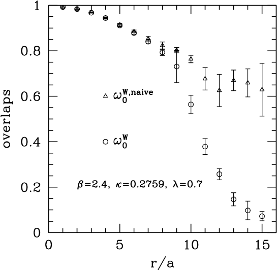
?figurename? 4.5: Here, we show the overlap $\omega_{0}^{\rm W}$ determined from the Wilson loops sub-block of the matrix correlation function. A “naive” way of extracting it (triangles), using eq. (4.29), gives an erroneous large overlap at long distances. A safe estimate (circles) is obtained from eq. (4.30).

It is interesting to consider also the overlap for the Wilson loops alone, i.e. we again restrict the matrix correlation function to the $3\times 3$ sub-block associated with (smeared) Wilson loops. Let us denote the corresponding projected correlation function by $\Omega_{\rm W}(t)$ and the overlap by $\omega_{0}^{\rm W}$. The computation of $\omega_{0}^{\rm W}$ is more difficult and tricky because it turns out to be very small at large $r$. In Fig. 4.5, we present the results for two estimates of $\omega_{0}^{\rm W}$. The triangles correspond to the estimate from eq. (4.29), with $\Omega(t)$ replaced by $\Omega_{\rm W}(t)$. The circles correspond to the more reliable estimate using the information from the full matrix correlation: the expression

$$\omega_{0}^{\rm W} {}_{\mbox{$\stackrel{{\scriptstyle\displaystyle\sim}}{{\scriptstyle t\rightarrow\infty}}$}} \omega_{0}{\Omega_{\rm W}(t)\over\Omega(t)}$$ (4.30)

converges reasonably fast and $\omega_{0}^{\rm W}$ can be estimated from the r.h.s. for large $t$. Using eq. (4.30), we see that (smeared) Wilson loops alone have an overlap which drops at intermediate distances and they are clearly inadequate to extract the ground state at large $r$. On the contrary, using eq. (4.29) we get an overlap above 50% at large distances: what is estimated here, is actually the coefficient $\omega_{1}^{\rm W}$, i.e. the overlap of the (smeared) Wilson loops with the first excited state (this statement is supported by direct calculation, see Sect. 4.2.5). Because $\omega_{1}^{\rm W}$ turns out to be so large, one should consider $\Omega_{\rm W}$ at much larger values of $t$ in order to extract the overlap $\omega_{0}^{\rm W}$ using eq. (4.29). This might explain the problems encountered in QCD for observing string breaking from the analysis of a correlation function with Wilson loops only.

4.2.5 Level crossing

Finally, we want to get an insight into the interplay between “string states” and “two-meson states” in the string breaking phenomenon. The results shown in Fig. 4.3 support the idea of crossing between the energy levels associated with these states. We try to quantify this statement.

We consider the diagonal sub-blocks of the matrix correlation function eq. (4.11) corresponding to string-type states (fields $i=1,2,3$ in eq. (4.10)) and to meson-type states (fields $i=4,5,...,12$ in eq. (4.10)) separately. We solve the generalised eigenvalue problem eq. (3.13) separately with these restricted matrix correlation functions for fixed $r$ and determine approximate ground state wave functions $v_{0}^{{\rm W}}$ for the string-type states and $v_{0}^{{\rm M}}$ for the meson-type states. With the help of these wave functions we construct a projected matrix correlation function

$$\Omega_{kl}(t)\,=\,v_{0,i}^{k}C_{ij}(t)v_{0,j}^{l}\,=\,\sum_{\alpha}\langle\psi_{l}|\alpha\rangle\langle\alpha|\psi_{k}\rangle{\rm e}^{-tV_{\alpha}(r)}\quad(k,l={\rm W},{\rm M})\,,$$ (4.31)

where

$$|\psi_{k}\rangle\;=\;\left(v_{0,i}^{k}\hat{{\rm O}}_{i}(r)\right)|0\rangle\,.$$ (4.32)

In eq. (4.32), the string-type ($k={\rm W}$) and meson-type ($k={\rm M}$) states are defined in terms of the operators that create them when applied to the vacuum $|0\rangle$. The definitions in eq. (4.32) follow directly from eq. (4.31) and eq. (4.11).

?figurename? 4.6: Here, the scalar product of the string-type and meson-type states defined in eq. (4.32) is shown as function of the separation $r$ of the static charges.

Taking $t=0$ in eq. (4.31), we get

$$\Omega_{kl}(0) = \langle\psi_{l}|\psi_{k}\rangle\,.$$ (4.33)

The projected matrix correlation in eq. (4.31) at time $t=0$ is equivalent to the scalar product of the states defined in eq. (4.32). From eq. (3.14), one convinces himself that the normalisation of the states $\langle\psi_{k}|\psi_{k}\rangle=1\;(k={\rm W},{\rm M})$ is a direct consequence of the solution of the generalised eigenvalue problem eq. (3.13) with $t_{0}=0$. The scalar product $\langle\psi_{{\rm M}}|\psi_{{\rm W}}\rangle$ is represented in Fig. 4.6 as a function of the separation $r$ of the static charges. We see that string-type and meson-type states are orthogonal only for large values of $r$.

?figurename? 4.7: Here, the overlaps of the string-type (circles) and meson-type (triangles) states, defined in eq. (4.32), with the ground state of the Hamiltonian are shown as functions of the separation $r$ of the static charges.

?figurename? 4.8: Here, the overlaps of the string-type (circles) and meson-type (triangles) states, defined in eq. (4.32), with the first excited eigenstate of the Hamiltonian are shown as functions of the separation $r$ of the static charges.

The coefficients

$$\omega_{k}(\alpha) \equiv \langle\alpha|\psi_{k}\rangle\quad(k={\rm W},{\rm M})\,,$$ (4.34)

in the expansion eq. (4.31), express the overlap of the string-type and meson-type states with the true eigenstates of the Hamiltonian. The matrix $\Omega_{kl}(t)$ is real, which means that the coefficients $\omega_{{\rm W}}(\alpha)$ and $\omega_{{\rm M}}(\alpha)$ have the same complex phase that can be absorbed into a redefinition of the state $|\alpha\rangle$. Therefore, we assume that the coefficients $\omega_{k}(\alpha)$ are real. Moreover, we can choose the sign conventions $\omega_{{\rm W}}(0)>0$ and $\omega_{{\rm W}}(1)>0$. We truncate the sum in eq. (4.31) after $\alpha=1$ and consider the diagonal matrix elements $\Omega_{kk}(t)$ for two fixed times $t=t_{1}$ and $t=t_{2}$: inserting the known values for $V_{0}(r)$ and $V_{1}(r)$, we get a linear system of equations for $\omega_{k}^{2}(0)$ and $\omega_{k}^{2}(1)$. The solutions read

$$\omega_{k}^{2}(0) = \frac{\Omega_{kk}(t_{1}){\rm e}^{t_{1}V_{1}(r)}-\Omega_{kk}(t_{2}){\rm e}^{t_{2}V_{1}(r)}}{{\rm e}^{t_{1}\Delta V(r)}-{\rm e}^{t_{2}\Delta V(r)}}\quad(k={\rm W},{\rm M})\,,$$ (4.35)

$$\omega_{k}^{2}(1) = {\rm e}^{t_{1}V_{1}(r)}[\Omega_{kk}(t_{1})-\omega_{k}^{2}(0){\rm e}^{-t_{1}V_{0}(r)}]\quad(k={\rm W},{\rm M})\,,$$ (4.36)

where $\Delta V(r)\equiv V_{1}(r)-V_{0}(r)$. The sign of the coefficients $\omega_{{\rm M}}(0)$ and $\omega_{{\rm M}}(1)$ is not fixed yet. From the solutions eq. (4.35) and eq. (4.36), we can compute the off-diagonal matrix elements $\Omega_{{\rm W}{\rm M}}(t_{1})$ and $\Omega_{{\rm W}{\rm M}}(t_{2})$ using eq. (4.31) for the four different sign combinations. Comparing with the values that we get from the simulation, we can establish the right sign combination. We find that for all $r$, $\omega_{{\rm M}}(0)>0$ and $\omega_{{\rm M}}(1)<0$ (in our sign convention). The overlaps eq. (4.35) and eq. (4.36) of the string-type (circles) and meson-type (triangles) states with the ground state of the Hamiltonian are shown in Fig. 4.7 and with the first excited eigenstate of the Hamiltonian in Fig. 4.8. The results correspond to the choice $t_{1}/a=5$ and $t_{2}/a=7$. Other choices of $t_{1}$ and $t_{2}$ give results which are compatible within the statistical errors. String-type states have a large overlap at short distances with the ground state and at large distances with the first excited state. Meson-type states have a large overlap at short distances with the first excited state and at large distances with the ground state. In addition, we observe that the overlap of the meson-type states with the ground state is also large at very short distances. The explanation for this fact is found by looking at Fig. 4.6, which clearly shows that string-type and meson-type states have an overlap with each other at short distances. In the string breaking region around $r/a=9-10$, the overlaps of the string-type and meson-type states have similar magnitude, both when the ground state or the first excited state is considered. This fact is reflected in the crossing of the energy levels Fig. 4.3. Here, we would like to point out that the overlaps represented in Fig. 4.7 and Fig. 4.8 are not quantities which have a continuum limit. They are specific to the $\beta$-value and the other parameters (e.g. of the smearing) that we consider.

?chaptername? 5 Scaling

The lattice spacing $a$ is mainly determined by the choice of the parameter $\beta=4/g^{2}$, where $g$ is the gauge coupling. Dimensionless physical quantities $F$ such as $F_{1}=r_{0}\,[2\mu-V_{0}(r_{0})]$ contain a dependence on the value of the lattice spacing which vanishes in the continuum limit. For a scalar theory we can write [80, 81]

$$F(a) = F(0)+{\rm O}\left((a/r_{0})^{2}\right)\,,$$ (5.1)

where ${\rm O}((a/r_{0})^{2})$ summarises terms that contain at least two powers of $a/r_{0}$ and may be modified by logarithmic corrections. When the corrections in eq. (5.1) (called lattice artifacts) become so small that $F$ is almost independent of $a$, we call this fact scaling. In order to investigate the presence of lattice artifacts in a dimensionless physical quantity, it is not sufficient to change the value of $\beta$ in a model with three bare parameters such as the SU(2) Higgs model. The physics of the model is influenced by the choice of all three parameters, for each observable differently. For an estimate of the correction terms in eq. (5.1) we must vary the lattice spacing $a$ (by changing $\beta$) and tune the bare parameters $\kappa$ and $\lambda$ to keep two dimensionless physical quantities $F_{1}$ and $F_{2}$ constant. This procedure corresponds to the renormalisation of $\kappa$ and $\lambda$ and defines in the parameter space a so called Line of Constant Physics (LCP) characterised by

$$F_{i}(\beta,\kappa,\lambda) = \mbox{constant},\quad i=1,2\,.$$ (5.2)

The situation is schematically represented in Fig. 5.1. Other dimensionless physical quantities $F_{3},\,F_{4},\,\cdot\cdot\cdot$ will, in principle, show correction terms as in eq. (5.1). This will give a measure for the scaling behavior of the theory in the investigated range of the lattice spacing.

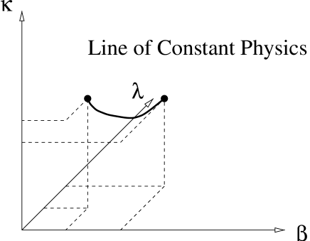
?figurename? 5.1: Here, a line of constant physics (LCP) in the SU(2) Higgs model is shown. The lattice spacing is changed along the LCP keeping two dimensionless physical quantities $F_{1}$ and $F_{2}$ at fixed values.

In Chapt. 3 and Chapt. 4 we presented results for the static-light meson spectrum and the static potentials obtained for the parameter set $\beta=2.4,\;\kappa=0.2759,\;\lambda=0.7$ on a $32^{4}$ lattice. We want to reproduce the physical situation on a coarser lattice corresponding to the choice $\beta=2.2$. A sensible choice for the dimensionless physical quantities to keep constant, would be to find $F_{1}$ strongly dependent on $\kappa$ and $F_{2}$ strongly dependent on $\lambda$. We have already found the right quantity $F_{1}=r_{0}\,[2\mu-V_{0}(r_{0})]$ eq. (4.26): it mainly depends on the value of the mass of the dynamical Higgs field which is in turn determined by the choice of $\kappa$. We now have to face the problem of finding $F_{2}$.

Physics shows a dependence on the physical size of the system and on the boundary conditions. We regularise the SU(2) Higgs model on a periodic lattice, which corresponds to a torus in the continuum and impose periodic boundary conditions on the fields. The physical lattice size $L/r_{0}$ is part of the definition of a dimensionless physical quantity $F$. The variation of the lattice spacing in eq. (5.1) must be accompanied by a change in the number of lattice points to keep the physical size of the torus constant. The dependence of a physical quantity on the size of the torus is called finite size effect.

It is well accepted – supported by the weak gauge coupling expansion [82] and by early numerical simulations [83, 84] – that the SU(2) Higgs model is a trivial theory [40], which means that the continuum limit is a free field theory. Nevertheless, the model can exhibit in a large range of values of the lattice spacing scaling properties of a non-trivial almost continuum theory. The interpretation of such a behavior is that the SU(2) Higgs model in this range describes an effective low-energy field theory and lattice results are perfectly relevant for a continuum Higgs model.

5.1 Matching of $\kappa$

Our choice of the first physical quantity to use for the matching of the bare parameters along the LCPs is $F_{1}=r_{0}\,[2\mu-V_{0}(r_{0})]$ eq. (4.26). The first matching condition reads

$$F_{1}\;=\;r_{0}\,[2\mu-V_{0}(r_{0})]\;=\;F_{1}^{*}\equiv 1.26\,,$$ (5.3)

where the numerical value is found at $\beta=2.4$ with a statistical error $\Delta F_{1}^{*}=0.02$. Since $F_{1}$ is mainly sensitive to the value of the meson mass $\mu$, which in turn is determined by the mass of the dynamical Higgs field, the quantity $F_{1}$ is surely sensitive to the parameter $\kappa$. For different values of $\lambda$, we match the parameter $\kappa$ at $\beta=2.2$ by computing $F_{1}$ on a $20^{4}$ lattice for two values $\kappa=\kappa_{1}$ (giving $F_{1}^{(1)}$ with statistical error $\Delta F_{1}^{(1)}$) and $\kappa=\kappa_{2}$ (giving $F_{1}^{(2)}$ with statistical error $\Delta F_{1}^{(2)}$). From a linear interpolation

$$F_{1}(\kappa)|_{\lambda} = a_{0}(\lambda)+\kappa\cdot a_{1}(\lambda)\,,$$ (5.4)

we determine $\kappa^{*}$ such that $F_{1}(\kappa^{*})=F_{1}^{*}$:

$$\kappa^{*} = \frac{\kappa_{1}(F_{1}^{*}-F_{1}^{(2)})+\kappa_{2}(F_{1}^{(1)}-F_{1}^{*})}{F_{1}^{(1)}-F_{1}^{(2)}}\,.$$ (5.5)

Propagating the independent errors $\Delta F_{1}^{(1)}$, $\Delta F_{1}^{(2)}$ and $\Delta F_{1}^{*}$, we get the error for the value $\kappa^{*}$ obtained from eq. (5.5).

?figurename? 5.2: Here, the matching of $\kappa$ at $\beta=2.2$ on a $20^{4}$ lattice using the condition eq. (5.3) is shown for different values of $\lambda$. The matched value $\kappa^{*}$ is obtained from eq. (5.5).

The results for $\lambda$=0.5, 0.55, 0.7, 0.757 are shown in Fig. 5.2. As a by-product of these simulations, we obtain the typical value of $r_{0}/a$ at $\beta=2.2$, for $F_{1}$ values near $F_{1}^{*}$:

$$r_{0}/a \approx 2.8\,.$$ (5.6)

Using eq. (4.22), we can derive the change in the lattice spacing between $\beta=2.2$ and $\beta=2.4$:

$${a(\beta=2.2)\over a(\beta=2.4)} \approx 1.9\,.$$ (5.7)

The choice of a $20^{4}$ lattice at $\beta=2.2$ and a $32^{4}$ lattice at $\beta=2.4$ corresponds only approximately to constant physical volume: we have $L/r_{0}\approx 7$ at $\beta=2.2$ and $L/r_{0}\approx 6$ at $\beta=2.4$. But these lattices can be considered relatively large for the extraction of the meson spectrum and the static potential: the relevant quantity, as we discussed in Sect. 3.1, is the product $Lm_{{\rm H}}$ which must be much larger than 1. The Higgs mass $m_{{\rm H}}$, that we define as the mass gap in the zero charge sector of the Hilbert space, can be estimated in our simulations to be $r_{0}m_{{\rm H}}\approx 1-1.5$, see Fig. 5.5. Therefore, we do not expect relevant finite size effects.

5.2 Matching of $\lambda$

In this section, we propose dimensionless physical quantities and study their $\lambda$ dependence. What we are looking for, are gauge invariant quantities with a well-defined continuum limit and sensitive to a variation of the parameter $\lambda$, once the parameter $\kappa$ is matched as described in Sect. 5.1.

In the region of small bare couplings, one can use bare lattice perturbation theory to determine the LCPs. By using an expansion for small gauge coupling one can derive, at the 1-loop level, the following equations [82]

$$\frac{{\rm d}\lambda_{0}(\tau)}{{\rm d}\tau} = \frac{1}{16\pi^{2}}\left[96\lambda_{0}^{2}+\frac{9}{32}g^{4}-9\lambda_{0}g^{2}+\cdot\cdot\cdot\right]\,,$$

$$\frac{{\rm d}g^{2}(\tau)}{{\rm d}\tau} = \frac{1}{16\pi^{2}}\left[-\frac{43}{3}g^{4}+\cdot\cdot\cdot\right]\,,$$ (5.8)

where $\tau\equiv\ln(am_{{\rm R}})^{-1}$ is the logarithm of the inverse of a renormalised mass in lattice units, $g^{2}=4/\beta$ and $\lambda_{0}=\lambda/(4\kappa^{2})$. The dots stand for terms of higher order ${\rm O}(\lambda_{0}^{3},\lambda_{0}^{2}g^{2},\lambda_{0}g^{4},g^{6})$.

The change $\tau_{2}-\tau_{1}=\ln(a_{1}/a_{2})$ in eq. (5.2) can be determined using eq. (5.7). If we then use eq. (5.2), with $\beta_{1}=2.2$ and $\lambda_{1}=0.5$ as initial conditions, to compute the change in $\lambda$ at $\beta_{2}=2.4$, we obtain the value $\lambda_{2}=0.8$, which is not far from the value $\lambda=0.7$ that we used for the simulations at $\beta=2.4$. The use of eq. (5.2) is not justified in this case, because the bare couplings are not small enough. Nevertheless, we take this crude estimate to start our investigations and we consider at $\beta=2.2$ the range $0.5\leq\lambda<0.8$.

5.2.1 Cumulants

We consider the gauge invariant Higgs field $S(x)=\Phi^{\dagger}(x)\Phi(x)$ and the construction of a renormalised coupling from its connected $p$-point (or Green) functions. There are some subtleties due to the fact that $S(x)$ is a composite field.

A composite field (or field operator) is a product of fields (field operators) at the same space-time point. The renormalisation of composite fields is a complicated issue and we refer to textbooks, e.g. [85, 86], for a detailed discussion. In general, a renormalised composite field $A_{{\rm R}}(x)$ is expressed in terms of unrenormalised fields $B(x)$ by

$$A_{{\rm R}}(x) = \sum_{B}Z_{AB}B(x)\,,$$ (5.9)

where $Z_{AB}$ are the renormalisation constants which depends on the bare couplings and on the cut-off, e.g. the lattice spacing $a$ in the lattice regularisation. The fields $B$, with which $A$ can mix under renormalisation, have canonical dimension equal to or lower than that of $A$ and the same quantum numbers of $A$. For example, the gauge invariant Higgs field $S(x)=\Phi^{\dagger}(x)\Phi(x)$ gets renormalised like

$$S_{{\rm R}}(x) = Z_{1}+Z_{S}S(x)\,.$$ (5.10)

The canonical dimension of the field $S(x)=\Phi^{\dagger}(x)\Phi(x)$ is two. Besides $1$ and $S(x)$ itself, there is no other gauge invariant scalar field of dimension two or less, with which $S(x)$ can mix under renormalisation.

The connected $p$-point (or Green) functions of $S(x)$ are defined by the path integral expectation values (see later)

$$G_{c}(x_{1},...,x_{p}) = \langle S(x_{1})\cdot\cdot\cdot S(x_{p})\rangle_{c}\,.$$ (5.11)

The renormalised connected $p$-point functions of $S(x)$, which we denote by $G_{c,{\rm R}}(x_{1},...,x_{p})$, are related to eq. (5.11) and eq. (5.10) by

$$G_{c,{\rm R}}(x_{1},...,x_{p})\;=\;\langle S_{{\rm R}}(x_{1})\cdot\cdot\cdot S_{{\rm R}}(x_{p})\rangle_{c}\;=\;Z_{S}^{p}\,G_{c}(x_{1},...,x_{p})\,,$$ (5.12)

The additive renormalisation $Z_{1}$ of the field $S(x)$ eq. (5.10) cancels in the definition of the connected Green functions. The multiplicative renormalisation factor $Z_{S}$ in eq. (5.10) is chosen so that the renormalised connected $p$-point functions in eq. (5.12) have a well-defined continuum limit, provided all points $x_{1},...,x_{p}$ are kept at non-zero distance from one another [87]. The question is, what happens in the continuum limit, if some of the points $x_{1},...,x_{p}$ coincide? This question can be addressed in the continuum with the help of the operator-product expansion of Wilson [88], according to which

$$\langle S_{{\rm R}}(x)S_{{\rm R}}(y)\rangle_{c} {}_{\mbox{$\stackrel{{\scriptstyle\displaystyle\sim}}{{\scriptstyle y\to x}}$}} \frac{1}{|x-y|^{4}}\,.$$ (5.13)

The power of the divergence on the right-hand side of eq. (5.13) corresponds to the naive dimensional counting. One can easily convince himself that this is true for free fields: for interacting fields, logarithmic correction factors may appear. We can generalise eq. (5.13) to the form

$$\langle S_{{\rm R}}(x_{1})\cdot\cdot\cdot S_{{\rm R}}(x_{k})\rangle_{c} {}_{\mbox{$\stackrel{{\scriptstyle\displaystyle\sim}}{{\scriptstyle x_{i}\to y}}$}} \frac{1}{|x-y|^{2k}}\quad(x\to y)\,.$$ (5.14)

We consider now the zero-momentum field

$$s_{{\rm R}} = \frac{1}{V}\int{\rm d}^{4}x\,S_{{\rm R}}(x)\,,$$ (5.15)

where $V$ is the physical volume of the torus. The connected $p$-point functions $\langle s_{{\rm R}}^{p}\rangle_{c}\;(p=2,3,4,...)$ can be written as

$$\langle s_{{\rm R}}^{p}\rangle_{c} = \frac{1}{V^{p}}\int{\rm d}^{4}x_{1}\cdot\cdot\cdot{\rm d}^{4}x_{p}\,\langle S_{{\rm R}}(x_{1})\cdot\cdot\cdot S_{{\rm R}}(x_{p})\rangle_{c}$$ (5.16)

$$= \frac{1}{V^{p-1}}\int{\rm d}^{4}y_{1}\cdot\cdot\cdot{\rm d}^{4}y_{p-1}\,\langle S_{{\rm R}}(y_{1})\cdot\cdot\cdot S_{{\rm R}}(y_{p-1})S_{{\rm R}}(0)\rangle_{c}\,,$$

where in the second line we used the translation invariance property of the connected Green functions. In naive dimensional counting, when $y_{i}\to 0\;(i=1,...,p-1)$, from the $(p-1)$ integrations we get $4(p-1)$ powers of $y$ whereas the integrand diverges in this limit like $|y|^{-2p}\,\;(y\to 0)$, as can be seen from eq. (5.14). Therefore, the $p$-point functions eq. (5.16) remain finite if

$$2p\;<\;4(p-1) \Leftrightarrow p\;>\;2\,.$$ (5.17)

Only the 2-point function $\langle s_{{\rm R}}^{2}\rangle_{c}$ is naively logarithmic divergent. This problem can be cured by defining a modified connected 2-point function

$$\langle\bar{s}^{(2)}_{{\rm R}}\rangle_{c} = \frac{1}{V}\int{\rm d}^{4}y\,\langle S_{{\rm R}}(y)S_{{\rm R}}(0)\rangle_{c}\,\sin\left(\frac{y_{0}}{T}\pi\right)$$ (5.18)

where $T$ is the time extension of the torus: throughout our work we use $T\equiv L\equiv V^{1/4}$. The sine function avoids contributions coming from $y=0$. In order to be sure that all divergencies associated with coincident arguments in eq. (5.16) are regularised for $p>2$, it remains to consider the case of two coincident arguments, e.g. $y_{1}\to y_{2}$. In contrast with $p=2$, there are still two integrations, over $y_{1}$ and $y_{2}$, that regulate the divergent behavior of the integrand, given in this limit by eq. (5.13). We are now able to give a definition of renormalised couplings in the continuum

$$c_{p} = \frac{\langle s^{p}\rangle_{c}}{\left[\langle\bar{s}^{(2)}\rangle_{c}\right]^{p/2}}\quad(p=3,4,5,...)\,.$$ (5.19)

The multiplicative renormalisation of the field $S(x)$ cancels in the ratio and we can then use the bare fields in eq. (5.19). We call the couplings defined by eq. (5.19) cumulants. We derive in the following expressions for the connected $p$-point functions of the zero-momentum field $s$.

In the path integral formalism the $p$-point functions $G(x_{1},...,x_{p})=\langle S(x_{1})\cdot\cdot\cdot S(x_{p})\rangle$ are constructed [89] from the generating functional

$$Z[J] = \langle\exp\{\int{\rm d}^{4}x\,J(x)S(x)\}\rangle$$ (5.20)

by functional differentiation with respect to the sources $J(x)$:

$$G(x_{1},...,x_{p}) = \left.\frac{\delta^{p}Z[J]}{\delta J(x_{1})\cdot\cdot\cdot\delta J(x_{p})}\right|_{J=0}\,.$$ (5.21)

Combining eq. (5.20) and eq. (5.21) we can write

$$Z[J] = \sum_{p=0}^{\infty}\frac{1}{n!}\int{\rm d}^{4}x_{1}\,...\,{\rm d}^{4}x_{p}\,J(x_{1})\cdot\cdot\cdot J(x_{p})\,G(x_{1},...,x_{p})\,.$$ (5.22)

The connected $p$-point functions $G_{c}(x_{1},...,x_{p})=\langle S(x_{1})\cdot\cdot\cdot S(x_{p})\rangle_{c}$ are constructed from the generating functional

$$W[J] = \ln\,Z[J]$$ (5.23)

in the same manner

$$G_{c}(x_{1},...,x_{p}) = \left.\frac{\delta^{p}W[J]}{\delta J(x_{1})\cdot\cdot\cdot\delta J(x_{p})}\right|_{J=0}\,.$$ (5.24)

Combining eq. (5.23) and eq. (5.24) we can write

$$W[J] = \sum_{p=0}^{\infty}\frac{1}{n!}\int{\rm d}^{4}x_{1}\,...\,{\rm d}^{4}x_{p}\,J(x_{1})\cdot\cdot\cdot J(x_{p})\,G_{c}(x_{1},...,x_{p})\,.$$ (5.25)

Expanding the right-hand side of eq. (5.23) in “powers” of $J$ one can derive general relations between $G_{c}$ and $G$. From these relations, we obtain that the connected $p$-point functions of $s$ can be expressed for $p=3,4,5$ by

$$\langle s^{3}\rangle_{c} = \langle s^{3}\rangle-3\langle s\rangle\langle s^{2}\rangle+2\langle s\rangle^{3}\,,$$ (5.26)

$$\langle s^{4}\rangle_{c} = \langle s^{4}\rangle-4\langle s^{3}\rangle\langle s\rangle-3\langle s^{2}\rangle^{2}+12\langle s^{2}\rangle\langle s\rangle^{2}-6\langle s\rangle^{4}\,,$$ (5.27)

$$\langle s^{5}\rangle_{c} = \langle s^{5}\rangle-5\langle s^{4}\rangle\langle s\rangle-10\langle s^{3}\rangle\langle s^{2}\rangle+20\langle s^{3}\rangle\langle s\rangle^{2}$$ (5.28)

$$+30\langle s^{2}\rangle^{2}\langle s\rangle-60\langle s^{2}\rangle\langle s\rangle^{3}+24\langle s\rangle^{5}\,.$$

Finally, we give a discretised version of the definition of the cumulants that we use on the lattice. The zero-momentum gauge invariant Higgs field is defined as

$$s = \frac{1}{\Omega}\sum_{x}S(x)\,,$$ (5.29)

where $\Omega$ is the number of lattice points. The cumulants are then defined as in eq. (5.19)

$$c_{p} = \frac{\langle s^{p}\rangle_{c}}{\left[\langle\bar{s}^{(2)}\rangle_{c}\right]^{p/2}}\quad(p=3,4,5,...)\,,$$ (5.30)

where the modified connected 2-point function $\langle\bar{s}^{(2)}\rangle_{c}$ is given by

$$\langle\bar{s}^{(2)}\rangle_{c} = \frac{1}{\Omega^{2}}\sum_{x,y}\langle S(x)S(y)\rangle_{c}\,\sin\left(\frac{x_{0}-y_{0}}{T}\pi\right)\,,$$ (5.31)

with $\langle S(x)S(y)\rangle_{c}=\langle S(x)S(y)\rangle-\langle S(x)\rangle\langle S(y)\rangle$. The connected $p$-point functions $\langle s^{p}\rangle_{c}\;(p=3,4,5)$ are computed according to eq. (5.26), eq. (5.27) and eq. (5.28) from the expectation values $\langle s^{q}\rangle\;(q=1,...,5)$.

Dependence on the volume

?figurename? 5.3: Here, we show the volume dependence of the cumulants $c_{3}$ and $c_{4}$ defined in eq. (5.30).

The cumulants $c_{p}$ for large values of $p$ are very small: in the Monte Carlo simulations we were able to obtain a significant signal up to $p=5$. In Fig. 5.3, we consider the volume dependence of $c_{3}$ and $c_{4}$ for the parameter set $\beta=2.4,\;\kappa=0.2759,\;\lambda=0.7$. We observe that the cumulants are strongly varying functions of the lattice size $L$: they are finite size couplings. The use of the cumulants for the matching of the parameters along the LCPs requires therefore a precise matching of the physical volume. We decided to compute the cumulants at $\beta=2.2$ on a $6^{4}$ lattice: the matching of the physical volume at $\beta=2.4$ using eq. (5.7) gives a lattice size $L/a\approx 11.4$.

Dependence on the parameter $\mathbf{\lambda}$

?figurename? 5.4: Here, we show the $\lambda$-dependence of the cumulants $c_{3}$ and $c_{4}$. The parameter $\kappa$ is matched such that $F_{1}=F_{1}^{*}$ eq. (5.3).

?figurename? 5.5: Here, we show the $\lambda$-dependence of the cumulant $c_{5}$ and the effective Higgs mass $Lm_{{\rm H}}^{\rm eff}(L/3)$. The parameter $\kappa$ is matched such that $F_{1}=F_{1}^{*}$ eq. (5.3).

In Fig. 5.4 and Fig. 5.5, we show the $\lambda$-dependence of the cumulants computed at $\beta=2.2$ on a $6^{4}$ lattice, with the parameter $\kappa$ matched such that $F_{1}=F_{1}^{*}$ eq. (5.3). In the interval of $\lambda$-values considered and within our statistical precision, the cumulants show a weak $\lambda$-dependence. Especially $c_{4}$ seems to be sensitive to $\lambda$. However, for the practical purpose of matching the $\lambda$ parameter, this situation is not suitable. As can be seen in Fig. 5.3, the cumulant $c_{4}$ computed at $\beta=2.4$ has a strong $L$-dependence in the region around the matched lattice size $L/a\approx 11.4$. The uncertainty coming from an interpolation to this lattice size and the statistical errors of $c_{4}$ at $\beta=2.2$ are the limiting factors for the matching of $\lambda$.

5.2.2 Higgs and W-boson correlations

We describe in the following the construction of renormalised quantities with a well-defined continuum limit from correlations of gauge invariant Higgs and W-boson fields with zero spacial momentum.

On each timeslice of the lattice, we construct a gauge invariant (composite) Higgs field with zero spacial momentum $H(x_{0})$ as follows:

$$H(x_{0}) = \left(\frac{a}{L}\right)^{3}\sum_{\vec{x}}\Phi^{\dagger}(x_{0},\vec{x})\Phi(x_{0},\vec{x})\,,$$ (5.32)

where the sum is over the points $\vec{x}$ in the timeslice with time coordinate $x_{0}$. We define the correlation function $f_{{\rm H}}(t)$ as

$$f_{{\rm H}}(t) = \frac{a}{T}\sum_{x_{0}}\langle H(x_{0}+t)H(x_{0})\rangle_{c}\,,$$ (5.33)

where $T$ denotes the time extent of the lattice: throughout our work we use $T\equiv L$. The connected expectation value of the product of two observables $O_{1}$ and $O_{2}$ is defined as usual by

$$\langle O_{1}\,O_{2}\rangle_{c} = \langle O_{1}\,O_{2}\rangle-\langle O_{1}\rangle\,\langle O_{2}\rangle\,.$$ (5.34)

The correlation function $f_{{\rm H}}(t)$ is multiplicatively renormalised with renormalisation factor $Z_{S}^{2}$ defined in eq. (5.10). Because the Higgs fields entering the connected two-point function in eq. (5.33) are taken at physical time separation $t$, the problems that we encountered in Sect. 5.2.1, due to the coincidence of the arguments of fields in Green functions, are avoided here. From the periodic boundary conditions in time direction, we derive the property $f_{{\rm H}}(T-t)=f_{{\rm H}}(t)$. The correlation function $f_{{\rm H}}(t)$ is symmetric with respect to the point $t=T/2$.

A gauge invariant W-boson field with zero spacial momentum is defined as

$$W_{rk}(x_{0}) = \left(\frac{a}{L}\right)^{3}\sum_{\vec{x}}-i\,\hbox{tr}\,(\tau_{r}V_{k}(x_{0},\vec{x}))\,,$$ (5.35)

where $V_{k}(x)\;(k=1,2,3)$ is the gauge invariant link defined in eq. (2.17) and $\tau_{r}\;(r=1,2,3)$ are the isospin Pauli matrices. We restrict the Lorentz index of the W-boson field to the spacial components $k$. We define the correlation function $f_{{\rm W}}(t)$ as

$$f_{{\rm W}}(t) = \frac{a}{T}\sum_{x_{0}}\sum_{r,k}\langle W_{rk}(x_{0}+t)W_{rk}(x_{0})\rangle_{c}\,.$$ (5.36)

The real field $W_{rk}(x)=-i\,\hbox{tr}\,(\tau_{r}V_{k}(x))$ corresponds in the naive continuum limit to the field $\,{\rm Re}\,\,\hbox{tr}\,(\tau_{r}\varphi^{\dagger}(x)D_{k}\varphi(x))$, where $D_{k}=\partial_{k}+igA_{kr}(x)\frac{\tau_{r}}{2}$ is the gauge covariant derivative for the gauge field $A_{kr}(x)$ and $\varphi(x)$ is the Higgs field in $2\times 2$ matrix notation. The canonical dimension of the field $W_{rk}(x)$ is therefore three and under renormalisation it can mix with fields of equal or lower canonical dimension which are gauge invariant and have an isospin index $r$ and a Lorentz index $k$. Because we are in a scalar theory we need a derivative $\partial_{k}$ to obtain a Lorentz index. The only possibility is the field $\partial_{k}\,\hbox{tr}\,(\tau_{r}\varphi^{\dagger}(x)\varphi(x))$, but it can be rewritten like $\,2{\rm Re}\,\,\hbox{tr}\,(\tau_{r}\varphi^{\dagger}(x)D_{k}\varphi(x))$. The absence of mixing with other fields implies that the correlation function $f_{{\rm W}}(t)$ is multiplicatively renormalised. Again, we have per construction the symmetry property $f_{{\rm W}}(T-t)=f_{{\rm W}}(t)$.

From the correlation functions $f_{i}(t),\;i={\rm H},{\rm W}$ we construct the quantities

$$\mu_{i}(t/T) = \ln\left(\frac{f_{i}(t)}{f_{i}(T/2)}\right)\,,\quad i={\rm H},{\rm W}\,.$$ (5.37)

The multiplicative renormalisation of the correlation functions cancels in the ratio and keeping the physical size $L\equiv T$ constant the $\mu_{i}$’s have a well-defined continuum limit.

Using the transfer matrix formalism it is easy to show that the correlation $f_{{\rm H}}(t)$ behaves like

$$f_{{\rm H}}(t) \sim {\rm const}\times\cosh\left((\frac{T}{2}-t)\,m_{{\rm H}}\right)\,,$$ (5.38)

where $m_{{\rm H}}\equiv E_{1}^{(0)}-E_{0}^{(0)}$. The energies $E_{\alpha}^{(0)}\;(\alpha=0,1,2,...)$ are the spectrum in the zero charge sector of the Hilbert space. We consider $m_{{\rm H}}$ to be the “Higgs mass” in the confinement phase of the model. The relation in eq. (5.38) is valid in the limits

$$t\,\Delta m_{{\rm H}}\gg 1 (T-t)\Delta m_{{\rm H}}\gg 1\,,$$ and (5.39)

where $\Delta m_{{\rm H}}\equiv E_{2}^{(0)}-E_{1}^{(0)}$. We can define an effective Higgs mass $m_{{\rm H}}^{\rm eff}(t)$ through the relation

$$\cosh\left((\frac{T}{2}-t)m_{{\rm H}}^{\rm eff}(t)\right) = \frac{f_{{\rm H}}(t)}{f_{{\rm H}}(T/2)}\,.$$ (5.40)

The effective mass $m_{{\rm H}}^{\rm eff}(t)$ converges for large enough $t$ to the Higgs mass $m_{{\rm H}}$. We could think to use $Lm_{{\rm H}}^{\rm eff}(t)$, determined at a fixed physical time $t$, as the dimensionless physical quantity $F_{2}$ for the matching of $\lambda$. In Fig. 5.5, we show the $\lambda$-dependence of $L\,m_{{\rm H}}^{\rm eff}(L/3)$ computed at $\beta=2.2$ on a $6^{4}$ lattice with the parameter $\kappa$ matched such that $F_{1}=F_{1}^{*}$ eq. (5.3). The effective mass is essentially a flat function of $\lambda$ within the statistical precision and it would not be suitable for the matching. The same conclusion is valid if we consider an effective mass extracted from the correlation function $f_{{\rm W}}(t)$. We note that these observations are in agreement with the exploratory results of reference [42].

5.3 Scaling

The results of Sect. 5.2, concerning the search for a dimensionless physical quantity $F_{2}$ which is sensitive to a variation of the parameter $\lambda$ once the parameter $\kappa$ is matched using the condition eq. (5.3), can be summarised in the following statements:

• The cumulant $c_{4}$, defined in eq. (5.30), shows a $\lambda$-dependence, as can be seen from Fig. 5.4. However, it is a strongly varying function of the lattice size, see Fig. 5.3. The use of $c_{4}$ for matching the parameter $\lambda$ requires a precise matching of the physical lattice size, which can be done only by interpolation and is therefore difficult.

• The Higgs and W-boson effective masses are essentially flat functions of $\lambda$, see Fig. 5.5.

In the following we use the assumption, supported by these results, that the physics in the confinement “phase” of the SU(2) Higgs model is weakly dependent on the parameter $\lambda$ once a dimensionless physical quantity such as $F_{1}=r_{0}\,[2\mu-V_{0}(r_{0})]$ is kept fixed. We compare the results for several dimensionless physical quantities computed at $\beta=2.2$ and at $\beta=2.4$ for the parameter sets

$$\beta=2.2,\qquad 0.5\leq\lambda<0.8,\qquad F_{1}(\kappa)=F_{1}^{*}\equiv 1.26$$ (5.41)

and

$$\beta=2.4,\qquad\lambda=0.7,\qquad\kappa=0.2759\,.$$ (5.42)

This comparison, by a change in the lattice spacing of almost a factor two eq. (5.7), gives a measure of the scaling properties of the SU(2) Higgs model in the confinement “phase”.

?figurename? 5.6: Here, we show the scaling of the logarithmic ratio $\mu_{{\rm H}}$ defined in eq. (5.37). The values at $\beta=2.2$ are computed with lattice size $L/r_{0}\approx 2.14$.

?figurename? 5.7: Here, we show the scaling of the logarithmic ratio $\mu_{{\rm W}}$ defined in eq. (5.37). The values at $\beta=2.2$ are computed with lattice size $L/r_{0}\approx 2.14$.

5.3.1 Cumulants

Because of the mentioned strong dependence of the cumulants on the physical lattice size and the difficulty to match it precisely between $\beta=2.2$ and $\beta=2.4$, we can only give some indications in form of the following table.

$$\begin{array}[]{lcl}\beta=2.2&&\beta=2.4\\ &&\\ c_{3}(L/r_{0}=2.12)\;=\;2.39(3)\quad(\lambda=0.5)&&c_{3}(L/r_{0}=2.08)\;=\;2.21(8)\\ c_{3}(L/r_{0}=2.16)\;=\;2.40(3)\quad(\lambda=0.7)&&c_{3}(L/r_{0}=2.27)\;=\;2.84(6)\\ &&\\ c_{4}(L/r_{0}=2.12)\;=\;1.77(11)\quad(\lambda=0.5)&&c_{4}(L/r_{0}=2.08)\;=\;1.9(3)\\ c_{4}(L/r_{0}=2.16)\;=\;2.08(13)\quad(\lambda=0.7)&&c_{4}(L/r_{0}=2.27)\;=\;5.1(3)\\ &&\\ c_{5}(L/r_{0}=2.12)\;=\;-9.3(4)\quad(\lambda=0.5)&&c_{5}(L/r_{0}=2.08)\;=\;-6.4(9)\\ c_{5}(L/r_{0}=2.16)\;=\;-7.6(5)\quad(\lambda=0.7)&&\end{array}$$

The numbers are compatible but no precise conclusion can be made.

5.3.2 Higgs and W-boson correlations

In Fig. 5.6 and Fig. 5.7 we show the results for the logarithmic ratios $\mu_{{\rm H}}$ and $\mu_{{\rm W}}$ defined in eq. (5.37). Because we cannot match exactly the physical size of the lattice, which at $\beta=2.2$ has the value $L/r_{0}\approx 2.14$, we show for $\beta=2.4$ the results for two different lattice sizes $L/r_{0}=1.89$ and $L/r_{0}=2.27$. Moreover, for $\beta=2.2$ we choose two values $\lambda=0.5$ and $\lambda=0.7$. The results show rough compatibility with scaling, even more pronounced for $\mu_{{\rm W}}$.

?figurename? 5.8: Here, we show the scaling of the renormalised ground state and first excited state static potentials.

?figurename? 5.9: Here, we show the $\lambda$-independence of the static potentials once the parameter $\kappa$ is matched by the condition $F_{1}=F_{1}^{*}$.

5.3.3 Static potentials

In Fig. 5.8, we compare the results for the renormalised ground state and first excited state static potentials that we obtained at $\beta=2.4$ (the same as in Fig. 4.3) and at $\beta=2.2,\;\kappa=0.2737,\;\lambda=0.5$. The results are compatible with scaling within minute errors! In Fig. 5.9, we compare the static potentials for two different values $\lambda=0.5$ and $\lambda=0.7$ at $\beta=2.2$. For $\lambda=0.7$ we use $\kappa=0.2928$. There is no significant difference, confirming the almost independence on $\lambda$ that we observed in Sect. 5.2.2 for the Higgs and W-boson mass. These results are a strong indication for a continuum-like behavior of the static potentials already at the small $\beta$ values that we use.

?chaptername? 6 Conclusions and Outlook

String breaking, the flattening of the static potential at large distances, is clearly observed in our lattice simulations of the four-dimensional SU(2) Higgs model in the confinement “phase”. We are able to determine the ground state and the first excited state static potentials with good precision. Our results confirm the interpretation of string breaking as a level crossing phenomenon between “string states” and “two-meson states”.

In the path integral formalism the static quarks are represented by straight time-like Wilson lines, the string-type states are represented by (smeared) space-like Wilson lines and the meson-type states by (smeared) Higgs fields. With these ingredients, a matrix correlation function can be constructed from which the static potentials are extracted using a variational method. We are able to describe the level crossing between the string-type and meson-type states in terms of the overlaps of these states with the true eigenstates of the Hamiltonian. In order to understand the difficulties in observing string breaking in recent lattice QCD simulations with dynamical fermions, we studied the extraction of the static potential from the string-type states (Wilson loops) alone. The overlap of the string-type states with the true ground state at large separations drops under 10%. The Wilson loops have in this region a large overlap with the first excited state. If we would extract the static potential from the Wilson loops alone we would see the continuation of the linear rise of the static potential beyond the expected asymptotic value, as observed in the QCD simulations [23, 24].

We addressed the question of the lattice artifacts in our results. The lines of constant physics (LCPs) in the parameter space of the SU(2) Higgs model are determined by the values of two dimensionless physical quantities $F_{1}$ and $F_{2}$: the lattice spacing is varied by changing $\beta$ and the bare parameters $\kappa$ and $\lambda$ are renormalised in order to keep $F_{1}$ and $F_{2}$ constant. The quantity $F_{1}$ that we choose is defined in eq. (4.26): it is mainly sensitive to the mass of the dynamical Higgs field and hence to $\kappa$. We studied then the sensitivity to $\lambda$ of different quantities. Our aim was to find a renormalised quartic Higgs coupling. We found a candidate, the cumulant $c_{4}$ defined in eq. (5.30), but no precise conclusions could be drawn. Our results support the conjecture that the physics in the confinement “phase” of the SU(2) Higgs model is weakly dependent on $\lambda$, once a physical quantity such as $F_{1}$ in eq. (4.26) is kept fixed. Assuming this, we studied the scaling behavior of different quantities between $\beta=2.2$ and $\beta=2.4$, for a variation of the lattice spacing by almost a factor of two. The ground state and first excited state static potentials are compatible with scaling within surprisingly small errors: our main result is shown in Fig. 5.8. Compatibility with scaling is also observed for the other quantities that we investigated.

The extension of the method described in [34] and in Sect. 4 of our work to QCD should present “only” problems related to statistical accuracy. There are two disadvantages in QCD with respect to our situation: there is no one-link integral to reduce the statistical variance of the correlations at large times and the computation of quark propagators is so CPU-time consuming that one cannot take advantage of translation invariance to reduce statistical errors as we did. On the other hand, in QCD the quark fields are integrated out analytically, which usually results in correlation functions with relatively small statistical errors. As concerns the computation of the quark propagators, the maximal variance reduction method of reference [90] is a promising prospective.

The search for a method of defining LCPs in the confinement “phase” of the SU(2) Higgs model is still an open and interesting question: the basic problem behind it, is to find a definition of a gauge invariant renormalised quartic Higgs coupling.

There are other important examples in QCD of phenomena involving mixing of states, like the computation of the glueball spectrum with dynamical fermions. The improvements that were made in the observation of string breaking can inspire the research in these other contexts.

?appendixname? A Notation conventions

A.1 Lattice notation

We consider in this work a four-dimensional hyper-cubic lattice in the Euclidean space with lattice spacing $a$

$$\Gamma = \{x/a\in{\mbox{\af N}}^{4}\,|\,a\leq x_{\mu}\leq L_{\mu},\;L_{0}\equiv T\}\,.$$ (A.1)

We use Greek symbols such as $\mu$, $\nu$, to denote all directions 0,1,2,3 and Roman symbols such as $k$ to denote the space-like directions 1,2,3. $\hat{\mu}$ is the unit vector in $\mu$ direction. The physical lattice volume is denoted by $V=TL_{1}L_{2}L_{3}$ and the number of lattice points by $\Omega=V/a^{4}$. The Fourier transformation of a function $f(x)$ on $\Gamma$ is defined by:

$$\tilde{f}(p) = a^{4}\sum_{x\in\Gamma}{\rm e}^{-ip\cdot x}f(x)\,,$$ (A.2)

where $p\cdot x\equiv p_{\mu}x_{\mu}\equiv\sum_{\mu}p_{\mu}x_{\mu}$. Considering periodic boundary conditions in all directions:

$$f(x+L_{\mu}\hat{\mu}) = f(x)\,,$$ (A.3)

the allowed lattice momenta are restricted to the first Brillouin zone

$${\mathcal{B}} = \{p\,|\,p_{\mu}=\frac{2\pi}{L_{\mu}}n_{\mu},\;n_{\mu}=0,1,...,L_{\mu}-1\}\,.$$ (A.4)

The inverse Fourier transformation of eq. (A.2) is

$$f(x) = \frac{1}{a^{4}\Omega}\sum_{p\in{\mathcal{B}}}{\rm e}^{ip\cdot x}\tilde{f}(p)\,.$$ (A.5)

A.2 SU($N$) gauge fields

A SU($N$) gauge field on the lattice is represented by the set of oriented links $U(x,\mu)_{ab}\in{\rm SU}(N)$ ($a,b=1,2,...,N$ are the color indices) connecting the points $x+a\hat{\mu}$ with $x$. A gauge transformation is defined by a field $\{\Lambda(x)\in{\rm SU}(N)\,|\,x\in\Gamma\}$ and by the transformations

$$U^{\Lambda}(x,\mu) = \Lambda^{\dagger}(x)U(x,\mu)\Lambda(x+a\hat{\mu})\,.$$ (A.6)

For the pure gauge theory, we use Wilson’s action which is based on the plaquette

$$P_{\mu\nu}(x) = U(x,\mu)U(x+a\hat{\mu},\nu)U^{\dagger}(x+a\hat{\nu},\mu)U^{\dagger}(x,\nu)$$ (A.7)

and reads

$$S_{{\rm W}} = \beta\sum_{x}\sum_{\mu<\nu}\left\{1-\frac{1}{N}{\rm Re}\,\,\hbox{tr}\,P_{\mu\nu}(x)\right\}\,.$$ (A.8)

For vanishing lattice spacing and smooth gauge fields, $S_{{\rm W}}$ reduces to the classical Yang-Mills action $S_{{\rm YM}}$ for gauge fields on the continuum

$$S_{{\rm W}} \longrightarrow S_{{\rm YM}}+{\rm O}(a^{2})\,,$$ (A.9)

if the bare gauge coupling constant $g$ on the lattice satisfies the relation

$$\beta = \frac{2N}{g^{2}}\,.$$ (A.10)

A.3 SU(2) Higgs field

A SU(2) Higgs field on the lattice is a complex scalar field $\Phi_{a}(x)\;(a=1,2)$ in the fundamental representation of the gauge group SU(2): under a gauge transformation $\{\Lambda(x)\in{\rm SU(2)}\,|\,x\in\Gamma\}$

$$\Phi^{\Lambda}(x) = \Lambda^{\dagger}(x)\Phi(x)\,.$$ (A.11)

$U(x,\mu)$ is the parallel transporter for the Higgs field, $U(x,\mu)\Phi(x+a\hat{\mu})$ transforms under gauge transformation like $\Phi(x)$. The lattice covariant derivative is defined as

$$\nabla_{\mu}\Phi(x) = \frac{1}{a}\,[U(x,\mu)\Phi(x+a\hat{\mu})-\Phi(x)]\,.$$ (A.12)

A peculiarity of the gauge group SU(2) is that the complex conjugate representation $2^{*}$ is equivalent to the fundamental representation $2$:

$$(i\tau_{2})^{-1}U(i\tau_{2}) = U^{*}\,,\quad U\in{\rm SU(2)}\,,$$ (A.13)

where $\tau_{r}\;(r=1,2,3)$ denote the Pauli matrices. This means that the field $\tilde{\Phi}(x)=i\tau_{2}\Phi^{*}(x)$ transforms like $\Phi(x)$. Using this property a representation by a $2\times 2$ matrix field $\varphi(x)$ can be constructed for the SU(2) Higgs field. We fix the notation

$$\Phi(x)=\left(\begin{array}[]{c}\Phi_{1}(x)=\phi_{1}(x)+i\phi_{2}(x)\\ \Phi_{2}(x)=\phi_{3}(x)+i\phi_{4}(x)\end{array}\right)\,,$$ (A.16)

where $\phi_{i}(x)\;(i=1,2,3,4)$ are the four real components of $\Phi(x)$, and we define

$$\varphi(x)=\left(\begin{array}[]{cc}\tilde{\Phi}_{1}(x)&\Phi_{1}(x)\\ \tilde{\Phi}_{2}(x)&\Phi_{2}(x)\end{array}\right)=\sqrt{\Phi^{\dagger}(x)\Phi(x)}\cdot\alpha(x)\,,$$ (A.19)

where $\alpha(x)\in{\rm SU(2)}$. Under gauge transformation $\varphi(x)$ transforms like

$$\varphi^{\Lambda}(x)=\Lambda^{\dagger}(x)\varphi(x)$$ (A.20)

The scalar product of two SU(2) doublets $\Phi$ and $\Psi$ can be written using the corresponding matrices $\varphi$ and $\psi$ constructed as in eq. (A.19):

$${\rm Re}\,\Phi^{\dagger}\Psi = \frac{1}{2}\,\hbox{tr}\,(\varphi^{\dagger}\psi)\,,$$ (A.21)

$${\rm Im}\,\Phi^{\dagger}\Psi = \frac{1}{2}\,\hbox{tr}\,((i\tau_{3})\varphi^{\dagger}\psi)\,.$$ (A.22)

?appendixname? B The transfer matrix in the SU(2) Higgs model

B.1 Hamiltonian formalism

Along the lines of reference [65] we construct a canonical, Hamiltonian formalism for fields living on a timeslice. We consider a three-dimensional lattice with sites $\vec{x}=a\cdot(n_{1},n_{2},n_{3}),\;n_{k}\in{\mbox{\af N}},\;1\leq k\leq 3,\;1\leq n_{k}\leq N$ and assume periodic boundary conditions. The Hilbert space $\hat{\cal H}$ is the set of all complex-valued, square-integrable wave functions $f$ with arguments $U(\vec{x},k)\in{\rm SU(2)}$ and $\Phi(\vec{x})\in{{\mbox{\af C}}}^{2}$ (in the following we shall denote them simply by $f(U,\Phi)$ or $|f\rangle$). The scalar product is defined by

$$\langle f|g\rangle = \int{\rm D}[U]\,{\rm D}[\phi]\,f(U,\Phi)^{*}\,g(U,\Phi)\,,$$ (B.1)

$$\int{\rm D}[U]\,{\rm D}[\phi]\, = \prod_{\vec{x},k}\int{\rm d}U(\vec{x},k)\cdot\prod_{\vec{x}}\int{\rm d}\phi_{1}(\vec{x})\cdot\cdot\cdot{\rm d}\phi_{4}(\vec{x})\,\,,$$ (B.2)

where ${\rm d}U$ is the Haar measure on SU(2) and $\phi_{i},\;i=1,2,3,4$ are the four real components of $\Phi$, see eq. (A.16). The field operators $\hat{\Phi}_{a}(\vec{x}),\;\hat{U}_{ab}(\vec{x},k)$ act as multiplicative operators on the wave functions $f$:

$$\left[\hat{U}_{ab}(\vec{x},k)\,f\right](U,\Phi) = U_{ab}(\vec{x},k)\,f(U,\Phi)\,,$$ (B.3)

$$\left[\hat{\Phi}_{a}(\vec{x})\,f\right](U,\Phi) = \Phi_{a}(\vec{x})\,f(U,\Phi)\,.$$ (B.4)

A gauge transformation is defined by a field of SU(2) matrices $\Lambda(\vec{x})$:

$$U^{\Lambda}(\vec{x},k) = \Lambda^{\dagger}(\vec{x})\,U(\vec{x},k)\,\Lambda(\vec{x}+a\hat{k})\,,$$ (B.5)

$$\Phi^{\Lambda}(\vec{x}) = \Lambda^{\dagger}(\vec{x})\,\Phi(\vec{x})\,.$$ (B.6)

In the Euclidean framework this corresponds to a time independent gauge transformation. In $\hat{\cal H}$ we define a unitary operator representation $\hat{\rm R}(\Lambda)$ such that

$$\left[\hat{\rm R}(\Lambda)\,f\right](U,\Phi) = f(U^{\Lambda},\Phi^{\Lambda})\,\equiv\,f^{\Lambda}(U,\Phi)\,.$$ (B.7)

Requiring gauge covariance of eq. (B.3) and eq. (B.4) one has

$$\hat{\rm R}^{\dagger}(\Lambda)\,\hat{U}_{ab}(\vec{x},k)\,\hat{\rm R}(\Lambda) = \Lambda^{\dagger}_{aa^{\prime}}(\vec{x})\,\hat{U}_{a^{\prime}b^{\prime}}(\vec{x},k)\,\Lambda_{b^{\prime}b}(\vec{x}+a\hat{k})\,,$$ (B.8)

$$\hat{\rm R}^{\dagger}(\Lambda)\,\hat{\Phi}_{a}(\vec{x})\,\hat{\rm R}(\Lambda) = \Lambda^{\dagger}_{aa^{\prime}}(\vec{x})\,\hat{\Phi}_{a^{\prime}}(\vec{x})\,.$$ (B.9)

An operator $\hat{{\rm O}}$ is called gauge invariant if

$$\left[\,\hat{\rm R}(\Lambda)\,,\,\hat{{\rm O}}\,\right] = 0\,.$$ (B.10)

In the following we shall need operators $\hat{{\rm O}}$ which can be represented with the help of an integral kernel $K_{{\rm O}}(U,\Phi;U^{\prime},\Phi^{\prime})$:

$$(\hat{{\rm O}}\,f)(U,\Phi) = \int{\rm D}[U^{\prime}]\,{\rm D}[\phi^{\prime}]\,K_{{\rm O}}(U,\Phi;U^{\prime},\Phi^{\prime})\,f(U^{\prime},\Phi^{\prime})\,.$$ (B.11)

The gauge invariance condition eq. (B.10) translates into

$$K_{{\rm O}}(U,\Phi;U^{\prime},\Phi^{\prime}) = K_{{\rm O}}(U^{\Lambda},\Phi^{\Lambda};U^{\prime\Lambda},\Phi^{\prime\Lambda})\,.$$ (B.12)

For the product of two operators $\hat{{\rm O}}_{1}\,\hat{{\rm O}}_{2}$ we have

$$K_{{\rm O}_{1}{\rm O}_{2}}(U,\Phi;U^{\prime},\Phi^{\prime}) = \int{\rm D}[U^{\prime\prime}]\,{\rm D}[\phi^{\prime\prime}]\,K_{{\rm O}_{1}}(U,\Phi;U^{\prime\prime},\Phi^{\prime\prime})\,\cdot$$

$$K_{{\rm O}_{2}}(U^{\prime\prime},\Phi^{\prime\prime};U^{\prime},\Phi^{\prime})\,.$$

The trace of an operator is defined as

$${\rm Tr}\,\hat{{\rm O}} = \int{\rm D}[U]\,{\rm D}[\phi]\,K_{{\rm O}}(U,\Phi;U,\Phi)\,.$$ (B.14)

B.2 The transfer matrix in the temporal gauge

We define an operator $\mathchoice{\rm T\kern-5.20004pt{T}}{\rm T\kern-5.20004pt{T}}{\rm T\kern-3.99994pt{T}}{\rm T\kern-3.99994pt{T}}_{\rm temp}$ through the following kernel:

$$K_{{\rm T}}^{\rm temp}(U,\Phi;U^{\prime},\Phi^{\prime}) = T_{{\rm H}}(U,\Phi)\cdot T_{{\rm G}}(U)\cdot S(U,\Phi;U^{\prime},\Phi^{\prime})\cdot$$

$$T_{{\rm G}}(U^{\prime})\cdot T_{{\rm H}}(U^{\prime},\Phi^{\prime})\,,$$

where

$$T_{{\rm G}}(U)=\exp\left\{-\frac{\beta}{2}\sum_{\vec{x}}\sum_{1\leq i<j\leq 3}\left[1-\frac{1}{2}\,\hbox{tr}\,P_{ij}(\vec{x})\right]\right\}\,$$ (B.16)

$$T_{{\rm H}}(U,\Phi)=\exp\left\{-\frac{1}{2}\sum_{\vec{x}}\Bigg{[}\lambda\left(\Phi^{\dagger}(\vec{x})\Phi(\vec{x})-1\right)^{2}\right.$$ (B.17)

$$\left.\left.-\kappa\sum_{k=1}^{3}\left(\Phi^{\dagger}(\vec{x})U(\vec{x},k)\Phi(\vec{x}+a\hat{k})+\Phi^{\dagger}(\vec{x}+a\hat{k})U^{\dagger}(\vec{x},k)\Phi(\vec{x})\right)\right]\right\}\,,$$

$$S(U,\Phi;U^{\prime},\Phi^{\prime})=\exp\left\{\sum_{\vec{x}}\Bigg{[}\kappa\left(\Phi^{\dagger}(\vec{x})\Phi^{\prime}(\vec{x})+\Phi^{\prime\dagger}(\vec{x})\Phi(\vec{x})\right)\right.$$ (B.18)

$$\left.\left.-\frac{1}{2}\left(\Phi^{\dagger}(\vec{x})\Phi(\vec{x})+\Phi^{\prime\dagger}(\vec{x})\Phi^{\prime}(\vec{x})\right)-\beta\sum_{k=1}^{3}\left(1-\frac{1}{2}\,\hbox{tr}\,(U(\vec{x},k)U^{\prime\dagger}(\vec{x},k))\right)\right]\right\}\,.$$

We included the terms quadratic in $\Phi$ and $\Phi^{\prime}$ separately, in $S$ eq. (B.18) instead of $T_{{\rm H}}$ eq. (B.17) for later convenience.

B.2.1 Positivity

Proposition 1.

• $\mathchoice{\rm T\kern-5.20004pt{T}}{\rm T\kern-5.20004pt{T}}{\rm T\kern-3.99994pt{T}}{\rm T\kern-3.99994pt{T}}_{\rm temp}$ is a selfadjoint, bounded and gauge invariant operator in $\hat{\cal H}$.

• $\mathchoice{\rm T\kern-5.20004pt{T}}{\rm T\kern-5.20004pt{T}}{\rm T\kern-3.99994pt{T}}{\rm T\kern-3.99994pt{T}}_{\rm temp}$ is strictly positive for $\kappa>0$ and $\lambda>0$
  (if $\lambda=0$ strict positivity holds for $0<\kappa<1/6$).

Selfadjointness of $K_{{\rm T}}^{\rm temp}$ means $K_{{\rm T}}^{\rm temp}(U^{\prime},\Phi^{\prime};U,\Phi)^{*}=K_{{\rm T}}^{\rm temp}(U,\Phi;U^{\prime},\Phi^{\prime})$. This follows from the fact that the kernel $K_{{\rm T}}^{\rm temp}$ is symmetric under interchange of $\{U,\Phi\}$ with $\{U^{\prime},\Phi^{\prime}\}$ and that the substitutions $U_{ab}(\vec{x})\rightarrow U_{ab}^{*}(\vec{x}),\;\Phi_{a}(\vec{x})\rightarrow\Phi_{a}^{*}(\vec{x})$ leave the integration measure and the action invariant.
In order for $K_{{\rm T}}^{\rm temp}$ to be bounded, one has to discuss the cases $\lambda>0$ and $\lambda=0$. If $\lambda>0$ the kernel is bounded for all values of $\kappa$ because of the term quartic in the Higgs field. If $\lambda=0$ one has to show that the matrix

$$B_{\vec{x}a,\vec{y}b} = \delta_{\vec{x},\vec{y}}\delta_{ab}-\kappa\sum_{k=1}^{3}\left[U_{ab}(\vec{x},k)\delta_{\vec{y},\vec{x}+a\hat{k}}+U^{\dagger}_{ab}(\vec{y},k)\delta_{\vec{x},\vec{y}+a\hat{k}}\right]$$ (B.19)

is strictly positive. This is the same as for fermionic fields [65]: the restriction $|\kappa|<1/6$ has to be imposed.
Gauge invariance of $K_{{\rm T}}^{\rm temp}$ (eq. (B.12)) is obvious.

To prove strict positivity of $\mathchoice{\rm T\kern-5.20004pt{T}}{\rm T\kern-5.20004pt{T}}{\rm T\kern-3.99994pt{T}}{\rm T\kern-3.99994pt{T}}_{\rm temp}$ one has to verify that

$$\int{\rm D}[U]\,{\rm D}[\phi]\,{\rm D}[U^{\prime}]\,{\rm D}[\phi^{\prime}]\,f(U,\Phi)^{*}\,K_{{\rm T}}^{\rm temp}(U,\Phi;U^{\prime},\Phi^{\prime})\,f(U^{\prime},\Phi^{\prime})$$

$$\equiv\;\langle f|\mathchoice{\rm T\kern-5.20004pt{T}}{\rm T\kern-5.20004pt{T}}{\rm T\kern-3.99994pt{T}}{\rm T\kern-3.99994pt{T}}_{\rm temp}|f\rangle\;>\;0\qquad\mbox{for all $f\neq 0$ in $\hat{\cal H}$.}$$ (B.20)

If $K_{{\rm T}}^{\rm temp}$ is bounded it is enough to show strict positivity for the kernel $S(U,\Phi;U^{\prime},\Phi^{\prime})$ because the kernels $T_{{\rm G}}$ and $T_{{\rm H}}$ can be absorbed in a new wave function $g=T_{{\rm G}}\,T_{{\rm H}}\,f\in\hat{\cal H}$. Furthermore, one has

$$S(U,\Phi;U^{\prime},\Phi^{\prime}) = \prod_{\vec{x}}S_{{\rm H}}(\Phi(\vec{x});\Phi^{\prime}(\vec{x}))\cdot\prod_{\vec{x},k}S_{{\rm G}}(U(\vec{x},k);U^{\prime}(\vec{x},k))\,,$$

$$S_{{\rm H}}(\Phi;\Phi^{\prime}) = \exp\left\{\kappa\left[\Phi^{\dagger}\Phi^{\prime}+\Phi^{\prime\dagger}\Phi\right]-\frac{1}{2}(\Phi^{\dagger}\Phi+\Phi^{\prime\dagger}\Phi^{\prime})\right\}\,,$$

$$S_{{\rm G}}(U;U^{\prime}) = \exp\left\{-\beta\left[1-\frac{1}{2}\,\hbox{tr}\,(UU^{\prime\dagger})\right]\right\}\,.$$

and we are left to prove that

$$\int{\rm d}U\,{\rm d}U^{\prime}\,{\rm d}^{4}\phi\,{\rm d}^{4}\phi^{\prime}\,h(U,\Phi)^{*}\,S_{{\rm H}}(\Phi;\Phi^{\prime})\,S_{{\rm G}}(U;U^{\prime})\,h(U^{\prime},\Phi^{\prime})\;>\;0\,$$ (B.21)

for all square integrable nonvanishing functions $h(U,\Phi)$ depending on one link variable $U$ and one field variable $\Phi$. Changing to the matrix notation for the Higgs field $\varphi=\rho\alpha,\;\rho\geq 0,\;\alpha\in{\rm SU(2)}$ one has

$$\Phi^{\dagger}\Phi^{\prime}+\Phi^{\prime\dagger}\Phi = \,\hbox{tr}\,(\varphi^{\dagger}\varphi^{\prime})\,,$$ (B.22)

$$\int_{\mathchoice{\rm I\kern-1.47005pt{R}}{\rm I\kern-1.47005pt{R}}{\rm I\kern-1.33002pt{R}}{\rm I\kern-1.33002pt{R}}^{4}}{\rm d}\phi_{1}(x)\cdot\cdot\cdot{\rm d}\phi_{4}(x) \propto \int_{0}^{\infty}\rho^{3}{\rm d}\rho\int_{{\rm SU(2)}}{\rm d}\alpha\,.$$ (B.23)

Expanding

$$\exp\{\kappa\,\hbox{tr}\,(\varphi^{\dagger}\varphi^{\prime})\} = \sum_{n=0}^{\infty}\frac{(\kappa\rho\rho^{\prime})^{n}}{n!}\left[\,\hbox{tr}\,(\alpha^{\dagger}\alpha^{\prime})\right]^{n}\,,$$

we recognise that $\left[\,\hbox{tr}\,(\alpha^{\dagger}\alpha^{\prime})\right]^{n}$ is the trace of the tensor product representation of SU(2) which is composed of n quarks[65]. Reducing out the tensor product we end up with

$$S_{{\rm H}}(\rho,\alpha;\rho^{\prime},\alpha^{\prime}) = \sum_{n=0}^{\infty}\frac{(\kappa\rho\rho^{\prime})^{n}}{n!}\sum_{\nu}b_{\nu}(n)\chi^{(\nu)}(\alpha^{\dagger}\alpha^{\prime})\cdot{\rm e}^{(\rho^{2}+\rho^{\prime 2})/2}\,.$$ (B.24)

$\nu$ labels the set of all inequivalent unitary irreducible representations of SU(2) and $\chi^{(\nu)}$ is the character of the representation $\nu$. The coefficient $b_{\nu}(n)$ is the number of times the representation $\nu$ occurs when reducing out the tensor product. Since all irreducible representations can be obtained in this way, for every $\nu$ exists a value of $n$ for which $b_{\nu}(n)\neq 0$. Similarly, the character expansion for $S_{{\rm G}}$ is [65]

$$S_{{\rm G}}(U;U^{\prime}) = {\rm e}^{-\beta}\cdot\sum_{\nu}c_{\nu}\chi^{(\nu)}(UU^{\prime\dagger})\,,\quad c_{\nu}>0\,.$$ (B.25)

Defining

$$h_{n}(U,\alpha) = \int_{0}^{\infty}{\rm d}\rho\,\rho^{3+n}\,h(U,\rho\alpha)\,{\rm e}^{-\rho^{2}/2}$$ (B.26)

and using the relation

$$\int{\rm d}U\,\chi^{(\nu)}(VU)\,\chi^{(\nu^{\prime})}(U^{\dagger}W) = \delta_{\nu\nu^{\prime}}\frac{1}{d_{\nu}}\chi^{(\nu)}(VW)\,,$$ (B.27)

where $d_{\nu}=\chi^{(\nu)}(\mathbf{1})$ is the dimension of the representation $\nu$, the integral in eq. (B.21) becomes

$$\sum_{\nu,\nu^{\prime}}\sum_{n}C(\nu,\nu^{\prime},n)\int{\rm d}V\,{\rm d}W\,\left|\int{\rm d}U{\rm d}\alpha\,h_{n}^{*}(U,\alpha)\,\chi^{(\nu)}(UV)\chi^{(\nu^{\prime})}(\alpha^{\dagger}W)\right|^{2}$$ (B.28)

where $C(\nu,\nu^{\prime},n)=d_{\nu}d_{\nu^{\prime}}c_{\nu}\kappa^{n}b_{\nu^{\prime}}(n){\rm e}^{-\beta}$. We are finally left with a sum of strictly positive terms provided $\kappa>0$.

One can show that the condition $\kappa>0$ is also necessary. It is possible to construct a function $h(U,\rho\alpha)=h(\rho)$ such that $h_{n}$ eq. (B.26) vanishes for all even $n$ and is different from zero for at least one odd $n_{0}$. If $\kappa$ is negative, for this function the whole sum eq. (B.28) is then negative.

B.3 Charge sectors

B.3.1 Minkowski space continuum

The classical Lagrange density for the SU(2) Higgs model in Minkowski space is

$${\cal L} = -\frac{1}{4}F_{a}^{\mu\nu}F_{a\mu\nu}+({\rm D}^{\mu}\Phi)^{\dagger}({\rm D}_{\mu}\Phi)-V(\Phi)\,,$$ (B.29)

$$F_{a}^{\mu\nu}(x) = \partial^{\mu}A^{\nu}_{a}(x)-\partial^{\nu}A_{a}^{\mu}(x)-g\varepsilon_{abc}A_{b}^{\mu}(x)A_{c}^{\nu}(x)\,,$$

$${\rm D}^{\mu}\Phi(x) = \left[\partial^{\mu}+igA_{a}^{\mu}(x)\frac{\tau_{a}}{2}\right]\Phi(x)\,,$$

$$V(\Phi(x)) = m_{0}^{2}\Phi^{\dagger}(x)\Phi(x)+\lambda_{0}[\Phi^{\dagger}(x)\Phi(x)]^{2}\,,$$

where the indices $a,b,c$ label the three generators of SU(2) $\frac{\tau_{a}}{2}$, $\tau_{a}$ being the Pauli matrices, and $g,\,m_{0},\;\mbox{and}\;\lambda_{0}$ are the bare couplings. The real vector fields $A_{a}^{\mu}$ carry a Lorentz index $\mu$ and a group index $a$. $\Phi$ is the complex Higgs SU(2) doublet field. The canonical conjugate momenta to the fields $A_{a}^{\mu}$ and $\Phi,\;\Phi^{\dagger}$ are

$$\Pi_{a}^{\mu}(x)=\frac{\partial{\cal L}}{\partial(\partial_{0}A_{a\mu}(x))} = -F_{a}^{\mu 0}(x)=\left\{\begin{array}[]{cl}-E_{a}^{i}&\mu=i=1,2,3\\ 0&\mu=0\end{array}\right.$$ (B.32)

$$\pi=\frac{\partial{\cal L}}{\partial(\partial_{0}\Phi(x))} = [{\rm D}^{0}\Phi(x)]^{\dagger}\,,$$ (B.33)

$$\pi^{\dagger}=\frac{\partial{\cal L}}{\partial(\partial_{0}\Phi^{\dagger}(x))} = {\rm D}^{0}\Phi(x)\,.$$ (B.34)

$E_{a}^{i}$ is the non-Abelian electric field strength. The generalisation of Gauss’ law follows from the equations of motion in the Lagrange formalism [91]:

$${\rm D}_{i}E^{i}_{a}\equiv\partial_{i}E^{i}_{a}+g\varepsilon_{abc}A_{b}^{i}E_{c}^{i} = j_{a}^{0}\,.$$ (B.35)

$j_{a}^{\mu}$ is the matter-field current and in particular

$$j_{a}^{0} = -ig\left[\pi\frac{\tau_{a}}{2}\Phi-\Phi^{\dagger}\frac{\tau_{a}}{2}\pi^{\dagger}\right]\,.$$ (B.36)

Performing the Legendre transformation to the Hamilton density one has to face the problem that the canonical conjugate momentum to $A^{0}_{a}$ is zero. One can choose a gauge in which the fields $A^{0}_{a}$ vanish identically, the temporal gauge [91]. There is still some freedom left in the choice of the gauge, namely the time independent gauge transformations. The canonical quantisation of the theory proceed considering wave functionals

$$\Psi[A_{a}^{i}(\vec{x}),\Phi(\vec{x})]$$ (B.37)

where the fields are taken at fixed time. In this representation of the states the field operators $\hat{A}_{a}^{i}(\vec{x})$ and $\hat{\Phi}(\vec{x})$ act as multiplicative operators and the conjugate momenta are represented by functional derivatives

$$\hat{E}_{a}^{i}(\vec{x}) = i\frac{\delta}{\delta A_{ai}(\vec{x})}\,,$$ (B.38)

$$\hat{\pi}(\vec{x}) = -i\frac{\delta}{\delta\Phi(\vec{x})}\,,$$ (B.39)

$$\hat{\pi}^{\dagger}(\vec{x}) = -i\frac{\delta}{\delta\Phi^{\dagger}(\vec{x})}\,.$$ (B.40)

Under a time independent gauge transformation $\Lambda(\vec{x})=\mathbf{1}-i\omega_{a}(\vec{x})\frac{\tau_{a}}{2}$ with infinitesimal parameters $\omega_{a}(\vec{x})$ the fields transform like:

$$\delta_{\Lambda}A_{a}^{i}(\vec{x}) = \frac{1}{g}\partial^{i}\omega_{a}(\vec{x})+\varepsilon_{abc}\omega_{b}(\vec{x})A_{c}^{i}(\vec{x})\,,$$ (B.41)

$$\delta_{\Lambda}\Phi(\vec{x}) = -i\omega_{a}(\vec{x})\frac{\tau_{a}}{2}\Phi(\vec{x})\,,$$ (B.42)

$$\delta_{\Lambda}\Phi^{\dagger}(\vec{x}) = i\omega_{a}(\vec{x})\Phi^{\dagger}(\vec{x})\frac{\tau_{a}}{2}\,.$$ (B.43)

Now, we would like to find the generators $\hat{{\rm G}}_{a}$ of the gauge transformations on the wave functionals $\Psi$:

$$\delta_{\Lambda}\Psi = -\frac{i}{g}\int{\rm d}^{3}x\,\omega_{a}(\vec{x})\,\hat{{\rm G}}_{a}(\vec{x})\Psi$$ (B.44)

To this aim we write:

$$\delta_{\Lambda}\Psi=\int{\rm d}^{3}x\left\{\frac{\delta\Psi}{\delta A_{ai}(\vec{x})}\delta_{\Lambda}A_{a}^{i}(\vec{x})+\frac{\delta\Psi}{\delta\Phi(\vec{x})}\delta_{\Lambda}\Phi(\vec{x})+\delta_{\Lambda}\Phi^{\dagger}(\vec{x})\frac{\delta\Psi}{\delta\Phi^{\dagger}(\vec{x})}\right\}$$

$$\qquad=-\frac{i}{g}\int{\rm d}^{3}x\,\omega_{a}(\vec{x})\bigg{\{}\left[\partial_{i}\hat{E}_{a}^{i}(\vec{x})+g\varepsilon_{abc}A_{b}^{i}(\vec{x})\hat{E}_{c}^{i}(\vec{x})\right]\Psi+$$

$$\qquad\quad ig\left[(\hat{\pi}(\vec{x})\Psi)\frac{\tau_{a}}{2}\Phi(\vec{x})-\Phi^{\dagger}(\vec{x})\frac{\tau_{a}}{2}(\hat{\pi}^{\dagger}(\vec{x})\Psi)\right]\bigg{\}}\,.$$ (B.45)

In the second line we used integration by part. From this we conclude that

$$\hat{{\rm G}}_{a}(\vec{x}) = {\rm D}_{i}\hat{E}^{i}_{a}(\vec{x})-\hat{j}^{0}_{a}(\vec{x})\,,$$ (B.46)

where the operators on the right hand side are defined by

$${\rm D}_{i}\hat{E}^{i}_{a}(\vec{x}) = \partial_{i}\hat{E}_{a}^{i}(\vec{x})+g\varepsilon_{abc}\hat{A}_{b}^{i}(\vec{x})\hat{E}_{c}^{i}(\vec{x})\,,$$

$$\hat{j}_{a}^{0}(\vec{x}) = -ig\left[\hat{\Phi}_{m}(\vec{x})\left(\frac{\tau_{a}}{2}\right)_{lm}\hat{\pi}_{l}(\vec{x})-\hat{\Phi}^{\dagger}(\vec{x})\frac{\tau_{a}}{2}\hat{\pi}^{\dagger}(\vec{x})\right]\,.$$

We can classify the wave functionals $\Psi$ according to the action of $\hat{{\rm G}}_{a}$. Gauss’ law

$$\hat{{\rm G}}_{a}\Psi = 0$$ (B.47)

is equivalent to the gauge invariance of the state $\Psi$. On states transforming like

$$\delta_{\Lambda}\Psi = -i\omega_{a}(\vec{x})T_{a}^{(\nu)}\Psi\,,$$ (B.48)

where $T_{a}^{(\nu)}$ are the generators of the irreducible representation $\nu$ of SU(2), the operator $\hat{G}$ acts as

$$\hat{{\rm G}}_{a}(\vec{x}^{\prime}) = gT_{a}^{(\nu)}\delta^{(3)}(\vec{x}-\vec{x}^{\prime})\,.$$ (B.49)

Thus wave functionals transforming under gauge transformation according to the representation $\nu$ of $\Lambda(\vec{x})$ for some fixed spacial point $\vec{x}$ express the presence of a static external charge at position $\vec{x}$ in the representation $\nu$.

B.3.2 Lattice formulation

Strict positivity of $\mathchoice{\rm T\kern-5.20004pt{T}}{\rm T\kern-5.20004pt{T}}{\rm T\kern-3.99994pt{T}}{\rm T\kern-3.99994pt{T}}_{\rm temp}$ allows the definition of an Hamiltonian $\mathchoice{\rm I\kern-1.4pt{H}}{\rm I\kern-1.4pt{H}}{\rm I\kern-1.1pt{H}}{\rm I\kern-1.1pt{H}}$:

$$\mathchoice{\rm I\kern-1.4pt{H}}{\rm I\kern-1.4pt{H}}{\rm I\kern-1.1pt{H}}{\rm I\kern-1.1pt{H}} = -\frac{1}{a}\ln\mathchoice{\rm T\kern-5.20004pt{T}}{\rm T\kern-5.20004pt{T}}{\rm T\kern-3.99994pt{T}}{\rm T\kern-3.99994pt{T}}_{\rm temp}$$ (B.50)

From the properties of $\mathchoice{\rm T\kern-5.20004pt{T}}{\rm T\kern-5.20004pt{T}}{\rm T\kern-3.99994pt{T}}{\rm T\kern-3.99994pt{T}}_{\rm temp}$ it follows that $\mathchoice{\rm I\kern-1.4pt{H}}{\rm I\kern-1.4pt{H}}{\rm I\kern-1.1pt{H}}{\rm I\kern-1.1pt{H}}$ is selfadjoint (has only real eigenvalues), bounded from below and gauge invariant.

The gauge symmetry of $\mathchoice{\rm I\kern-1.4pt{H}}{\rm I\kern-1.4pt{H}}{\rm I\kern-1.1pt{H}}{\rm I\kern-1.1pt{H}}$ allows to choose its eigenstates with a well defined transformation property under the gauge group. The Hilbert space $\hat{\cal H}$ can then be classified according to the irreducible representations of SU(2) on each point of the lattice [92]. As we saw inspecting Gauss’ law in the continuum these representations define the charge sectors of $\hat{\cal H}$. The transfer matrix is restricted to a specific charge sector by multiplying it with the projector $\mathchoice{\rm I\kern-1.4pt{P}}{\rm I\kern-1.4pt{P}}{\rm I\kern-1.1pt{P}}{\rm I\kern-1.1pt{P}}$ onto this sector. We give two examples of charge sectors which are of interest for us.

The zero charge sector (vacuum sector) corresponds to the gauge invariant wave functions. We denote by $|n_{0}\rangle$ the eigenstates of $\mathchoice{\rm I\kern-1.4pt{H}}{\rm I\kern-1.4pt{H}}{\rm I\kern-1.1pt{H}}{\rm I\kern-1.1pt{H}}$ with eigenvalues $E_{n}^{(0)}$ which form a basis of this sector. The corresponding projection operator $\mathchoice{\rm I\kern-1.4pt{P}}{\rm I\kern-1.4pt{P}}{\rm I\kern-1.1pt{P}}{\rm I\kern-1.1pt{P}}_{0}=\sum_{n_{0}}|n_{0}\rangle\langle n_{0}|$ is

$$(\mathchoice{\rm I\kern-1.4pt{P}}{\rm I\kern-1.4pt{P}}{\rm I\kern-1.1pt{P}}{\rm I\kern-1.1pt{P}}_{0}\,f)(U,\Phi) = \int\prod_{\vec{z}}{\rm d}\,W(\vec{z})\,f^{W}(U,\Phi)\,.$$ (B.51)

The transfer matrix operator in the zero charge sector is $\mathchoice{\rm T\kern-5.20004pt{T}}{\rm T\kern-5.20004pt{T}}{\rm T\kern-3.99994pt{T}}{\rm T\kern-3.99994pt{T}}_{0}=\mathchoice{\rm T\kern-5.20004pt{T}}{\rm T\kern-5.20004pt{T}}{\rm T\kern-3.99994pt{T}}{\rm T\kern-3.99994pt{T}}_{\rm temp}\mathchoice{\rm I\kern-1.4pt{P}}{\rm I\kern-1.4pt{P}}{\rm I\kern-1.1pt{P}}{\rm I\kern-1.1pt{P}}_{0}$ and has the kernel

$$K_{{\rm T}}^{0}(U,\Phi;U^{\prime},\Phi^{\prime}) = \int\prod_{\vec{z}}{\rm d}\,W(\vec{z})\,K_{{\rm T}}^{\rm temp}(U,\Phi;U^{\prime W^{\dagger}},\Phi^{\prime W^{\dagger}})$$ (B.52)

A wave function $f$ in the sector of $\hat{\cal H}$ with a static quark at position $\vec{x}$ and a static anti-quark at position $\vec{y}$ transforms as

$$f^{\Lambda}_{ab} = \sum_{a^{\prime},b^{\prime}=1}^{2}\Lambda_{aa^{\prime}}(\vec{x})\,f_{a^{\prime}b^{\prime}}\,\Lambda^{\dagger}_{b^{\prime}b}(\vec{y})$$ (B.53)

We choose a basis $|n_{{\rm q}\bar{{\rm q}}},a,b\rangle$ with eigenvalues $E_{n}^{({\rm q}\bar{{\rm q}})}$ of $\mathchoice{\rm I\kern-1.4pt{H}}{\rm I\kern-1.4pt{H}}{\rm I\kern-1.1pt{H}}{\rm I\kern-1.1pt{H}}$ independent of $a,b$. We drop in the following the color indices $a,b$ of the states when an implicit sum over them is meant. The projection operator $\mathchoice{\rm I\kern-1.4pt{P}}{\rm I\kern-1.4pt{P}}{\rm I\kern-1.1pt{P}}{\rm I\kern-1.1pt{P}}(\vec{x},\vec{y})=\sum_{n_{{\rm q}\bar{{\rm q}}}}|n_{{\rm q}\bar{{\rm q}}}\rangle\langle n_{{\rm q}\bar{{\rm q}}}|$ onto this sector is

$$(\mathchoice{\rm I\kern-1.4pt{P}}{\rm I\kern-1.4pt{P}}{\rm I\kern-1.1pt{P}}{\rm I\kern-1.1pt{P}}(\vec{x},\vec{y})\,f)(U,\Phi)\,=\,\int\prod_{\vec{z}}{\rm d}\,W(\vec{z})\,4\,\,\hbox{tr}\,W^{\dagger}(\vec{x})\,\,\hbox{tr}\,W(\vec{y})\,f^{W}(U,\Phi)\,.$$ (B.54)

The transfer matrix operator in this sector is $\mathchoice{\rm T\kern-5.20004pt{T}}{\rm T\kern-5.20004pt{T}}{\rm T\kern-3.99994pt{T}}{\rm T\kern-3.99994pt{T}}_{{\rm q}(\vec{x}),\bar{{\rm q}}(\vec{y})}=\mathchoice{\rm T\kern-5.20004pt{T}}{\rm T\kern-5.20004pt{T}}{\rm T\kern-3.99994pt{T}}{\rm T\kern-3.99994pt{T}}_{\rm temp}\mathchoice{\rm I\kern-1.4pt{P}}{\rm I\kern-1.4pt{P}}{\rm I\kern-1.1pt{P}}{\rm I\kern-1.1pt{P}}(\vec{x},\vec{y})$ and has the kernel

$$K_{{\rm T}}^{{\rm q}\bar{{\rm q}}}(U,\Phi;U^{\prime},\Phi^{\prime}) = \int\prod_{\vec{z}}{\rm d}\,W(\vec{z})\,4\,\,\hbox{tr}\,W^{\dagger}(\vec{x})\,\,\hbox{tr}\,W(\vec{y})\,\cdot$$ (B.56)

$$K_{{\rm T}}^{\rm temp}(U,\Phi;U^{\prime W^{\dagger}},\Phi^{\prime W^{\dagger}})\,.$$

B.4 Reconstruction of the Euclidean expectation values

We consider operators $\hat{{\rm O}}(\vec{x},\vec{y})_{ab}$ which transform under gauge transformation according to

$$\hat{\rm R}^{\dagger}(\Lambda)\hat{{\rm O}}(\vec{x},\vec{y})_{ab}\hat{\rm R}(\Lambda) = \Lambda^{\dagger}_{aa^{\prime}}(\vec{x})\hat{{\rm O}}(\vec{x},\vec{y})_{a^{\prime}b^{\prime}}\Lambda_{b^{\prime}b}(\vec{y})\,.$$ (B.57)

These operators create out of the vacuum states belonging to the sector with a static pair of quarks. Examples are:

$$\hat{\Phi}_{a}(\vec{x})\,\hat{\Phi}_{b}^{\dagger}(\vec{y})\quad\mbox{and}\quad\hat{U}(\vec{x},\vec{y})_{ab}$$ (B.58)

$U(\vec{x},\vec{y})$ denotes the product of links along a path connecting $\vec{y}$ with $\vec{x}$. Because of eq. (B.3) and eq. (B.4) we can directly associate the observables $O(\vec{x},\vec{y})_{ab}=\Phi_{a}(\vec{x})\Phi_{b}^{*}(\vec{y})$ and $U(\vec{x},\vec{y})_{ab}$.

B.4.1 Reconstruction theorem

Proposition 2.

• $${\rm Tr}(\mathchoice{\rm T\kern-5.20004pt{T}}{\rm T\kern-5.20004pt{T}}{\rm T\kern-3.99994pt{T}}{\rm T\kern-3.99994pt{T}}_{0}^{M})=\prod_{x,\mu}\int{\rm d}U(x,\mu)\cdot\prod_{x}\int{\rm d}\phi_{1}(x)\cdot\cdot\cdot{\rm d}\phi_{4}(x)\,\exp(-S)\equiv Z$$

  is the partition function on a four-dimensional lattice with time coordinate $x_{0}/a=1,2,...,M$ and periodic boundary conditions.

• $${\rm Tr}\left(\sum_{b,c}\hat{{\rm B}}(\vec{x},\vec{y})^{\dagger}_{cb}\mathchoice{\rm T\kern-5.20004pt{T}}{\rm T\kern-5.20004pt{T}}{\rm T\kern-3.99994pt{T}}{\rm T\kern-3.99994pt{T}}_{{\rm q}(\vec{x}),\bar{{\rm q}}(\vec{y})}^{t/a}\hat{{\rm A}}(\vec{x},\vec{y})_{bc}\mathchoice{\rm T\kern-5.20004pt{T}}{\rm T\kern-5.20004pt{T}}{\rm T\kern-3.99994pt{T}}{\rm T\kern-3.99994pt{T}}_{0}^{M-t/a}\right)\,/\,{\rm Tr}(\mathchoice{\rm T\kern-5.20004pt{T}}{\rm T\kern-5.20004pt{T}}{\rm T\kern-3.99994pt{T}}{\rm T\kern-3.99994pt{T}}_{0}^{M})$$

  
  

  $$=\langle\,\hbox{tr}\,\left(A(x,y)U(y,y+t\hat{0})B(x+t\hat{0},y+t\hat{0})^{\dagger}U(x,x+t\hat{0})^{\dagger}\right)\rangle\equiv C_{{\rm A}{\rm B}}$$

  
  

  where $x_{0}=y_{0}$ and $\hat{{\rm A}},\hat{{\rm B}}$ are operators of the type of eq. (B.57). This is the amplitude for the transition from the state $A$ to the state $B$ over a time interval $t$.

We first inspect the kernel of $\mathchoice{\rm T\kern-5.20004pt{T}}{\rm T\kern-5.20004pt{T}}{\rm T\kern-3.99994pt{T}}{\rm T\kern-3.99994pt{T}}_{0}$ in eq. (B.52). Identifying $W(\vec{z})$ with the time-like links $U(z,0),\;z=(z_{0},\vec{z})$, renaming $\Phi^{\prime}(\vec{z})\rightarrow\Phi(z+a\hat{0})$ and $U^{\prime}(\vec{z},k)\rightarrow U(z+a\hat{0},k)$ we see that eq. (B.18), excluding the terms quadratic in $\Phi$ and $\Phi^{\prime}$ separately, becomes

$$S(U,\Phi;U^{\prime W^{\dagger}},\Phi^{\prime W^{\dagger}}) = \exp\{-\Delta S(z_{0},z_{0}+a)\}\,.$$ (B.59)

$\Delta S(z_{0},z_{0}+a)$ are the terms in the action which couples variables on the neighboring timeslices $t=z_{0}$ and $t=z_{0}+a$. From this we see that the integration over the time-like links in the path integral is equivalent to the projection onto the gauge invariant sector of $\hat{\cal H}$. eq. (B.59) is also the reason why we called $\mathchoice{\rm T\kern-5.20004pt{T}}{\rm T\kern-5.20004pt{T}}{\rm T\kern-3.99994pt{T}}{\rm T\kern-3.99994pt{T}}_{\rm temp}$ the transfer matrix in the temporal gauge. The other factors in $K_{{\rm T}}^{\rm temp}$ contain the pieces of the action depending only on the fields in the timeslices and the trace is equivalent to the periodic boundary conditions in the time direction.

The numerator of the left hand side of b) can be written as

$$\prod_{z,\mu}\int_{{\rm SU(2)}}{\rm d}U(z,\mu)\cdot\prod_{z}\int_{\mathchoice{\rm I\kern-1.47005pt{R}}{\rm I\kern-1.47005pt{R}}{\rm I\kern-1.33002pt{R}}{\rm I\kern-1.33002pt{R}}^{4}}{\rm d}^{4}\phi(z)\,\,\hbox{tr}\,\left(A(x,y)B(x+t\hat{0},y+t\hat{0})^{\dagger}\right)\,\cdot$$

$$2^{t/a}\,\,\hbox{tr}\,U^{\dagger}(x+(t-a)\hat{0},0)\,\,\hbox{tr}\,U^{\dagger}(x+(t-2a)\hat{0},0)\,\cdot\cdot\cdot\,\,\hbox{tr}\,U^{\dagger}(x,0)\,\cdot$$

$$2^{t/a}\,\,\hbox{tr}\,U(y,0)\,\,\hbox{tr}\,U(y+a\hat{0},0)\,\cdot\cdot\cdot\,\hbox{tr}\,U(y+(t-a)\hat{0},0)\,\cdot$$

$$\exp(-S)\,.$$ (B.60)

Because the action and the measure are gauge invariant, for any observable $O$ one has $\langle O^{\Lambda}\rangle=\langle O\rangle$, where $O^{\Lambda}$ is the gauge transformed observable. Gauge transforming eq. (B.4.1), integrating over $\prod_{w_{0}=x_{0}}^{x_{0}+t}\int\prod_{\vec{w}}{\rm d}\,\Lambda(w_{0},\vec{w})$ and applying eq. (B.27) one sees that the product of traces in eq. (B.4.1) is glued into one trace, the right hand side of b).

B.4.2 The static potential

Using the spectral decomposition $\mathchoice{\rm T\kern-5.20004pt{T}}{\rm T\kern-5.20004pt{T}}{\rm T\kern-3.99994pt{T}}{\rm T\kern-3.99994pt{T}}_{0}=\sum_{n_{0}}|n_{0}\rangle\exp(-aE_{n}^{(0)})\langle n_{0}|$ the partition function can be written as

$$Z = \sum_{n_{0}}\exp\left\{-MaE_{n}^{(0)}\right\}\,.$$ (B.61)

Inserting $\mathchoice{\rm T\kern-5.20004pt{T}}{\rm T\kern-5.20004pt{T}}{\rm T\kern-3.99994pt{T}}{\rm T\kern-3.99994pt{T}}_{{\rm q}(\vec{x}),\bar{{\rm q}}(\vec{y})}=\sum_{n_{{\rm q}\bar{{\rm q}}}}|n_{{\rm q}\bar{{\rm q}}}\rangle\exp(-aE_{n}^{({\rm q}\bar{{\rm q}})})\langle n_{{\rm q}\bar{{\rm q}}}|$ in the quantum mechanical expression for the correlation $C_{{\rm A}{\rm B}}$ we have:

$$C_{{\rm A}{\rm B}} = \frac{1}{Z}\sum_{n_{0},n_{{\rm q}\bar{{\rm q}}}}\left(\sum_{b,c}\langle n_{0}|\hat{{\rm B}}^{\dagger}_{cb}|n_{{\rm q}\bar{{\rm q}}}\rangle\langle n_{{\rm q}\bar{{\rm q}}}|\hat{{\rm A}}_{bc}|n_{0}\rangle\right)\cdot$$

$$\exp\left\{-t(E_{n}^{({\rm q}\bar{{\rm q}})}-E_{n}^{(0)})\right\}\cdot\exp\left\{-MaE_{n}^{(0)}\right\}$$

In the limit of $Ma-t\gg 1/m_{1}^{(0)}$, where $m_{1}^{(0)}$ is the mass gap in the gauge invariant sector, and $t\gg(E_{1}^{({\rm q}\bar{{\rm q}})}-E_{0}^{({\rm q}\bar{{\rm q}})})^{-1}$ we have the asymptotic behavior

$$C_{{\rm A}{\rm B}} \sim \alpha_{\rm B}^{*}\,\alpha_{\rm A}\,\exp\left\{-t(E_{0}^{({\rm q}\bar{{\rm q}})}-E_{0}^{(0)})\right\}\,,$$ (B.63)

where $\alpha_{\rm A}=\langle 0_{{\rm q}\bar{{\rm q}}}|\hat{{\rm A}}|0\rangle$ and the trace over the color indices of the states and operators is implicit. The quantity

$$V = E_{0}^{({\rm q}\bar{{\rm q}})}-E_{0}^{(0)}$$ (B.64)

is called the static potential.

?appendixname? C Updating algorithms

In this appendix, we give a detailed description of the algorithms that we used for the Monte Carlo simulation of the SU(2) Higgs model on the lattice. Before describing the algorithms, we want to discuss the generation of random numbers which are an essential part of the updating.

C.1 Random Numbers

Because the updating process is stochastic, one needs to generate a large number of independent random numbers. We use the high-quality random number generator of M. Lüscher [93, 94], derived from an algorithm originally proposed by Marsaglia and Zaman [95]. It generates random floating point numbers distributed uniformly in the range $[0,1)$. From these flat random numbers we have to construct random numbers with probability distributions needed in the updating of the gauge and Higgs field variables.

To be clear with the terminology, one speaks in general of random numbers $\eta$ distributed in an interval $[a,b]\subset\mathchoice{\rm I\kern-2.10007pt{R}}{\rm I\kern-2.10007pt{R}}{\rm I\kern-1.90002pt{R}}{\rm I\kern-1.90002pt{R}}$ with probability density $p(\eta)$. The normalisation of the density is such that $\int_{a}^{b}p(\eta)\,{\rm d}\eta=1$. A uniform (or flat) distribution of a random number $\eta$ in the interval $[a,b]$ corresponds to $p(\eta)=1/(b-a)$. The probability distribution $P(\eta)$ is related to the probability density by

$$\frac{{\rm d}P(\eta)}{{\rm d}\eta} = p(\eta)\,.$$ (C.1)

If one considers a transformation of variable $\tilde{\eta}=b(\eta)$ the probability density $\tilde{p}(\tilde{\eta})$ of the transformed variable is related to $p(\eta)$ by the requirement

$${\rm d}P(\eta) = {\rm d}\tilde{P}(\tilde{\eta})\,.$$ (C.2)

First of all, we consider the generation of random numbers $\tilde{\eta}$ distributed according to the Gaussian density

$$\tilde{p}(\tilde{\eta}) = \frac{1}{\sqrt{\pi}}{\rm e}^{-\tilde{\eta}^{2}}\,.$$ (C.3)

It is better to consider the generation of a couple $(\tilde{\eta}_{1},\tilde{\eta}_{2})$ of independent Gaussian random numbers. Independent means that

$${\rm d}\tilde{P}(\tilde{\eta}_{1},\tilde{\eta}_{2}) = \tilde{p}(\tilde{\eta}_{1}){\rm d}\tilde{\eta}_{1}\,\tilde{p}(\tilde{\eta}_{2}){\rm d}\tilde{\eta}_{2}\,.$$ (C.4)

With the variable transformations $\tilde{\eta}_{1}=\rho\cos\theta$ and $\tilde{\eta}_{2}=\rho\sin\theta$, where $\rho\in[0,\infty)$ and $\theta\in[0,2\pi)$ we can rewrite eq. (C.4) using eq. (C.2) as

$${\rm d}P(\rho,\theta) = {\rm d}\tilde{P}(\tilde{\eta}_{1},\tilde{\eta}_{2})\;=\;\frac{1}{\pi}\rho{\rm e}^{-\rho^{2}}{\rm d}\rho{\rm d}\theta$$ (C.5)

$$= {\rm d}\left(1-{\rm e}^{-\rho^{2}}\right)\,{\rm d}\left(\frac{\theta}{2\pi}\right)\,.$$

This is equivalent to the generation of a couple $(\eta_{1},\eta_{2})$ of independent flat random numbers in the range $[0,1)$ together with the transformations $\eta_{1}=1-\exp(-\rho^{2})$ and $\eta_{2}=\theta/(2\pi)$. The final result is then

$$\tilde{\eta}_{1} = \sqrt{-\ln(1-\eta_{1})}\cos(2\pi\eta_{2})\quad\mbox{and}$$

$$\tilde{\eta}_{2} = \sqrt{-\ln(1-\eta_{1})}\sin(2\pi\eta_{2})\,.$$ (C.6)

Gaussian random numbers are needed in the updating of the Higgs field variables, see Sect. C.3.1.

Secondly, we consider the generation of random numbers distributed in $[0,\infty)$ according to the density

$$p(y) = \frac{2}{\sqrt{\pi}}\sqrt{y}\exp(-y)\Theta(y)\,,$$ (C.7)

where

$$\Theta(x-x_{0}) = \left\{\begin{array}[]{ll}1&\mbox{for}\quad x>x_{0}\\ 0&\mbox{for}\quad x<x_{0}\end{array}\right.$$ (C.10)

is the Heaviside function. This can be done by generating a number $a\in[0,\infty)$ according to the Gaussian density

$$p(a) = \frac{2}{\sqrt{\pi}}{\rm e}^{-a^{2}}\Theta(a)$$ (C.11)

and independently a number $b\in[0,\infty)$ with the exponential density

$$p(b) = {\rm e}^{-b}\Theta(b)\,.$$ (C.12)

To generate $a$ one uses eq. (C.1) replacing $2\pi\eta_{2}$ with $\pi\eta_{2}/2$ as the argument for the trigonometric functions. To generate $b$ one simply takes a flat distributed random number $\eta$ in the range $[0,1)$ and sets $b=-\ln(1-\eta)$. We define the variables

$$\bar{y}\;=\;a y\;=\;a^{2}+b$$ and (C.13)

with ranges $y\in[0,\infty)$ and $\bar{y}\in[0,\sqrt{y})$. From eq. (C.2) we get the relation

$${\rm d}P(\bar{y},y) = {\rm d}P(a,b)\;=\;\frac{2}{\sqrt{\pi}}{\rm e}^{-y}\Theta(\bar{y})\Theta(\sqrt{y}-\bar{y}){\rm d}\bar{y}{\rm d}y\,,$$ (C.14)

which means that the variables $\bar{y}$ and $y$ are distributed with probability density $p(\bar{y},y)=2/\sqrt{\pi}\exp(-y)\Theta(\bar{y})\Theta(\sqrt{y}-\bar{y})$. The probability density for $y$ alone is obtained by integrating $p(\bar{y},y)$ over all possible values of $\bar{y}$:

$$p(y) = \int_{0}^{\sqrt{y}}\frac{2}{\sqrt{\pi}}{\rm e}^{-y}\Theta(y){\rm d}\bar{y}\;=\;\frac{2}{\sqrt{\pi}}\sqrt{y}{\rm e}^{-y}\Theta(y)\,.$$ (C.15)

The random numbers $y$ from eq. (C.13) are needed in the updating of the gauge link variables, see Sect. C.2.1.

Now, we are ready to describe the different parts of the HOR algorithm introduced in Sect. 2.4.

C.2 Updating of the gauge field

To discuss the updating of the link variable $U(x,\mu)$, we split the action eq. (2.1) into

$$S = -\frac{\beta}{2}\,\hbox{tr}\,\{U(x,\mu)W^{\dagger}(x,\mu)\}+$$ (C.16)

$$\mbox{terms independent of $U(x,\mu)$}\,,$$

$$W(x,\mu) = V(x,\mu)+\frac{2\kappa}{\beta}\varphi(x)\varphi^{\dagger}(x+a\hat{\mu})\,,$$ (C.17)

where $V(x,\mu)$ is the sum of the products of links over the six “staples” around the link $U(x,\mu)$

$$V(x,\mu) = \sum_{\nu\neq\mu}\{U(x,\nu)U(x+a\hat{\nu},\mu)U^{\dagger}(x+a\hat{\mu},\nu)+$$ (C.18)

$$\quad U^{\dagger}(x-a\hat{\nu},\nu)U(x-a\hat{\nu},\mu)U(x-a\hat{\nu}+a\hat{\mu},\nu)\}\,.$$

We denote the part of the action depending on $U(x,\mu)$ in eq. (C.17) by $S(U(x,\mu))$.

C.2.1 Heatbath

The heatbath algorithm for the gauge field in the SU(2) Higgs model is a simple modification of the algorithm for the pure SU(2) gauge theory [96, 97, 98]. We drop the arguments $(x,\mu)$ of the link to be updated. The new link $U^{\prime}$ is chosen independently of $U$ according to the Boltzmann distribution

$${\rm d}P(U^{\prime}) \sim {\rm e}^{\frac{\beta}{2}\,\hbox{tr}\,(U^{\prime}W^{\dagger})}\,{\rm d}U^{\prime}\,.$$ (C.19)

The matrix $W$ defined in eq. (C.17) can be written as $W=\sqrt{\det W}\,\hat{W}$, where $\hat{W}\in{\rm SU(2)}$. Using the invariance of the Haar measure we obtain from eq. (C.19)

$${\rm d}P(U^{\prime}\hat{W}) \sim {\rm e}^{\frac{1}{2}\rho\,\hbox{tr}\,(U^{\prime})}\,{\rm d}U^{\prime}\,,$$ (C.20)

where $\rho=\beta\sqrt{\det W}$. Writing $U^{\prime}$ in the quaternionic representation

$$U^{\prime}=a_{0}+ia_{j}\tau_{j}\quad,\quad a_{\mu}\in\mathchoice{\rm I\kern-2.10007pt{R}}{\rm I\kern-2.10007pt{R}}{\rm I\kern-1.90002pt{R}}{\rm I\kern-1.90002pt{R}}\quad,\quad a^{2}=a_{\mu}a_{\mu}=1\,,$$ (C.21)

where $\tau_{j}\;(j=1,2,3)$ are the Pauli matrices, the Haar measure for SU(2) takes the form [40] ${\rm d}U^{\prime}=\frac{1}{\pi^{2}}\delta(a^{2}-1){\rm d}^{4}a$ and eq. (C.20) becomes

$${\rm d}P(U^{\prime}\hat{W}) \sim \frac{1}{\pi^{2}}\delta(a^{2}-1){\rm e}^{\rho a_{0}}\,da_{0}d^{3}a\,.$$ (C.22)

The heatbath algorithm consists then in the following:

1. Generation of $a_{\mu}$ according to the distribution

   $${\rm d}P(a_{\mu}) \sim \sqrt{1-a_{0}^{2}}{\rm e}^{\rho a_{0}}{\rm d}a_{0}\,{\rm d}^{3}n\delta(n^{2}-1)\,,$$ (C.23)

   where $a_{j}=n_{j}\sqrt{1-a_{0}^{2}}$. This is done using the method described in [98] which is a slight variation of that of Fabricius and Haan [96]. In order to generate $a_{0}\in[-1,1]$ with the distribution

   $${\rm d}P(a_{0}) \sim \sqrt{1-a_{0}^{2}}{\rm e}^{\rho a_{0}}{\rm d}a_{0}$$ (C.24)

   we perform the change of variable

   $$y = \rho(1-a_{0})\in[0,2\rho]\,.$$ (C.25)

   According to eq. (C.2) we rewrite eq. (C.24) as

   $${\rm d}P(y) \sim (2-\frac{y}{\rho})^{1/2}\sqrt{y}{\rm e}^{-y}{\rm d}y\,.$$ (C.26)

   The generation of random numbers $y$ according to eq. (C.26) cannot be done exactly. Instead, one generates $y$ according to the probability density eq. (C.7) as explained in Sect. C.1. An accept-reject step takes into account the omitted factor $(2-\frac{y}{\rho})^{1/2}$. A flat random number $\eta\in[0,1)$ is generated: if

   $$2\eta^{2} \leq 2-\frac{y}{\rho}$$ (C.27)

   the change $a_{0}=1-y/\rho$ is accepted. We notice that the values $y>2\rho$ are automatically rejected in eq. (C.27). The components $n_{j}$ of the vector $n$ in eq. (C.23) are uniformly distributed on the surface of the unit sphere in three dimensions. The generation of $n_{j}$ requires two flat distributed random numbers $\eta_{1}$ and $\eta_{2}$ in the interval [0,1):

   $$n_{1} = 1-2\eta_{1}\,,$$ (C.28)

   $$n_{2} = \sqrt{1-n_{1}^{2}}\cos(2\pi\eta_{2})\,,$$ (C.29)

   $$n_{3} = \sqrt{1-n_{1}^{2}}\sin(2\pi\eta_{2})\,.$$ (C.30)

2. If eq. (C.27) is fulfilled, $U$ is substituted by

   $$U^{\prime}\hat{W}\;=\;\frac{1}{\sqrt{\det W}}U^{\prime}W\,.$$ (C.31)

Simulating the SU(2) Higgs model on a $12^{4}$ lattice with parameters $\beta=2.0$, $\kappa=0.25$ and $\lambda=0.5$ (this point is in the confinement “phase”) the change eq. (C.31) is accepted in 95% of the cases.

C.2.2 Overrelaxation

The new link $U$ proposed is

$$U^{\prime} = \hat{W}U^{\dagger}\hat{W}\;=\;\frac{1}{\det W}WU^{\dagger}W$$ (C.32)

This change is microcanonical, i.e. $S(U)=-\rho/2\,\hbox{tr}\,(U\hat{W}^{\dagger})=S(U^{\prime})$ because of the reality of the trace of SU(2) elements. Since the inverse relation of eq. (C.32) is $U=\hat{W}U^{\prime\dagger}\hat{W}$, eq. (C.32) is a reflection of $U$ and $U^{\prime}$ and therefore the factors $p_{\rm C}$ cancel in the acceptance probability eq. (2.29). The change eq. (C.32) is always accepted.

C.3 Updating of the Higgs field

For the updating of the Higgs field we use the algorithms proposed in [53]. In particular the over-relaxation algorithm has been proved to be very efficient for the reduction of autocorrelations.

The part of the SU(2) Higgs model action eq. (2.1) depending on the Higgs field reads

$$S_{\phi} = \sum_{x}\left\{\frac{1}{2}\,\hbox{tr}\,(\varphi^{\dagger}(x)\varphi(x))+\lambda\left[\frac{1}{2}\,\hbox{tr}\,(\varphi^{\dagger}(x)\varphi(x))-1\right]^{2}\right.$$ (C.33)

$$\left.-\kappa\sum_{\mu}\,\hbox{tr}\,(\varphi^{\dagger}(x)U(x,\mu)\varphi(x+\hat{\mu}))\right\}\,.$$

Combining eq. (A.16) and eq. (A.19) the $2\times 2$ matrix $\varphi$ can be written in terms of the four real components $\phi_{i}(x)\;(i=1,2,3,4)$ as

$$\varphi(x) = \left(\begin{array}[]{cc}\phi_{3}(x)-i\phi_{4}(x)&\phi_{1}(x)+i\phi_{2}(x)\\ -\phi_{1}(x)+i\phi_{2}(x)&\phi_{3}(x)+i\phi_{4}(x)\end{array}\right)\,.$$ (C.36)

If we do the same for the matrix

$$B(x) = \kappa\sum_{\mu}\left[U(x,\mu)\varphi(x+\hat{\mu})+U^{\dagger}(x-\hat{\mu},\mu)\varphi(x-\hat{\mu})\right]$$ (C.39)

$$= \left(\begin{array}[]{cc}b_{3}(x)-ib_{4}(x)&b_{1}(x)+ib_{2}(x)\\ -b_{1}(x)+ib_{2}(x)&b_{3}(x)+ib_{4}(x)\end{array}\right)\quad b_{i}\in\mathchoice{\rm I\kern-2.10007pt{R}}{\rm I\kern-2.10007pt{R}}{\rm I\kern-1.90002pt{R}}{\rm I\kern-1.90002pt{R}}\,,$$

we can write the action eq. (C.33) in the four component notation of reference [53]

$$S_{\phi}=\sum_{x}\left\{(\phi(x)-b(x))^{2}+\lambda\left[\phi^{2}(x)-1\right]^{2}-b^{2}(x)\right\}\,,$$ (C.40)

where the squares mean the scalar product in $\mathchoice{\rm I\kern-2.10007pt{R}}{\rm I\kern-2.10007pt{R}}{\rm I\kern-1.90002pt{R}}{\rm I\kern-1.90002pt{R}}^{4}$.

C.3.1 Heatbath

We drop the index $i$ and the argument $x$ of the Higgs field variable $\phi_{i}(x)\;(i=1,2,3,4)$ to be updated. A new Higgs variable $\phi^{\prime}$ has to be generated according to the distribution

$${\rm d}P(\phi^{\prime})\;\sim\;{\rm e}^{-V(\phi^{\prime})}\,{\rm d}^{4}\phi^{\prime}\quad,\quad V(\phi)=(\phi-b)^{2}+\lambda(\phi^{2}-1)^{2}\,.$$ (C.41)

This is best achieved by introducing a free parameter $\alpha$ which parametrises the splitting of the potential $V(\phi)$ in a quadratic and in a quartic part

$$V(\phi) = \alpha(\phi-\alpha^{-1}b)^{2}+\lambda(\phi^{2}-v_{\alpha}^{2})^{2}-c_{\alpha}\,,$$ (C.42)

where

$$v_{\alpha}^{2} = 1+\frac{\alpha-1}{2\lambda}\,,$$ (C.43)

$$c_{\alpha} = \lambda(v_{\alpha}^{4}-1)+(\alpha^{-1}-1)b^{2}\,.$$ (C.44)

A trial Higgs variable is generated according to the Gaussian density (see eq. (C.1))

$$p_{\rm trial}(\phi^{\prime}) = \left(\frac{\alpha}{\pi}\right)^{2}{\rm e}^{-\alpha(\phi^{\prime}-\alpha^{-1}b)^{2}}$$ (C.45)

and is accepted with probability

$$w_{\rm acpt}(\phi^{\prime}) = {\rm e}^{-\lambda(\phi^{\prime 2}-v_{\alpha}^{2})^{2}}\,.$$ (C.46)

The parameter $\alpha$ is chosen so that it maximises the acceptance rate defined as

$$A(\alpha) = \int{\rm d}^{4}\phi\,p_{\rm trial}(\phi)w_{\rm acpt}(\phi)\,,$$ (C.47)

which can be rewritten using eq. (C.42) as

$$A(\alpha) = \alpha^{2}{\rm e}^{-c_{\alpha}}A(1)\,.$$ (C.48)

Differentiating with respect to $\alpha$ yields the cubic equation

$$f(\alpha)\equiv\alpha^{3}-(1-2\lambda)\alpha^{2}-4\lambda\alpha = 2\lambda b^{2}\,.$$ (C.49)

The exact solution of eq. (C.49) is inconvenient because the dependence on $b^{2}$ forces to solve it separately for each update. We use the approximate solution proposed in [99]. The function $f(\alpha)$ in eq. (C.49) vanishes at

$$\alpha_{0} = \frac{1}{2}-\lambda+\left[(\frac{1}{2}-\lambda)^{2}+4\lambda\right]^{1/2}\,.$$ (C.50)

Expanding $f(\alpha)$ in powers of $(\alpha-\alpha_{0})$ and omitting the cubic term, eq. (C.49) becomes

$$(\alpha_{0}^{2}+4\lambda)(\alpha-\alpha_{0})+(6\alpha_{0}+4\lambda-2)\frac{1}{2}(\alpha-\alpha_{0})^{2} = 2\lambda b^{2}\,.$$ (C.51)

The positive solution of eq. (C.51) is

$$\alpha = h_{0}+[h_{1}+h_{2}\,b^{2}]^{1/2}\,,$$ (C.52)

with

$$h_{0} = \alpha_{0}-\frac{\alpha_{0}^{2}+4\lambda}{6\alpha_{0}+4\lambda-2}\,,$$ (C.53)

$$h_{1} = \left(\frac{\alpha_{0}^{2}+4\lambda}{6\alpha_{0}+4\lambda-2}\right)^{2}\,,$$ (C.54)

$$h_{2} = \frac{4\lambda}{6\alpha_{0}+4\lambda-2}\,.$$ (C.55)

The constants $\alpha_{0}$ and $h_{i}\;(i=0,1,2)$ can be computed in advance because they do not depend on $b$. For the update of $\phi$ it is only necessary to determine $b$, find $\alpha$ according to eq. (C.52) and the corresponding $v_{\alpha}^{2}$ from eq. (C.43). Simulating the SU(2) Higgs model for relatively large value of $\lambda$, the choice $\alpha=1$, corresponding to a naive splitting of the potential $V(\phi)$ in eq. (C.42), would lead to a low acceptance $A(1)$ in eq. (C.48). Using eq. (C.52) we get values $A=70\%$ in the confinement “phase” ($\beta=2.0$, $\kappa=0.25$, $\lambda=0.5$) and $A=59\%$ in the Higgs “phase” ($\beta=2.3$, $\kappa=0.32$, $\lambda=1.0$), both the simulations performed on a $12^{4}$ lattice.

C.3.2 Overrelaxation

The following change of the Higgs variable is proposed [53]:

$$\phi \longrightarrow \phi^{\prime}=2\alpha^{-1}b-\phi\,.$$ (C.56)

This change is not microcanonical, but it is a reflection of $\phi$ and $\phi^{\prime}$, since the inverse relation of eq. (C.56) is $\phi=2\alpha^{-1}b-\phi^{\prime}$. According to eq. (2.29) the new Higgs variable is accepted with a probability

$$p_{\rm A} = \min\left\{1,\exp\left[V(\phi)-V(\phi^{\prime})\right]\right\}$$ (C.57)

$$= \min\left\{1,\exp\left[\lambda(\phi^{2}-\phi^{\prime 2})(\phi^{2}+\phi^{\prime 2}-2v_{\alpha}^{2})\right]\right\}\,.$$

For the acceptance $A$ of the change eq. (C.56) we get values $A=79\%$ in the confinement “phase” ($\beta=2.0$, $\kappa=0.25$, $\lambda=0.5$) and $A=68\%$ in the Higgs “phase” ($\beta=2.3$, $\kappa=0.32$, $\lambda=1.0$), both the simulations performed on a $12^{4}$ lattice.

?appendixname? D One-link integral and approximation of the modified Bessel functions

In Sect. 3.2, we presented a method for reducing the statistical variance of correlation functions involving static charges which are represented in the path integral formalism by straight time-like Wilson lines. The time-like links can be replaced (with some restriction) by their expectation value (called one-link integral) in the fixed configuration of the other field variables.

First of all, we present the derivation of the result eq. (3.19). We omit writing the $(x,0)$ dependence of $U$ and $W$, for the rest the notation is the same as in Sect. 3.2. We denote by $\hat{W}$ the projection $W/\sqrt{\det(W)}$ of $W$ into SU(2). The one-link integral can be written after a change of integration variable as

$$\overline{U} = \frac{\int{\rm d}U\,U\,\exp\{(\rho/2)\,\hbox{tr}\,(U)\}}{\int{\rm d}U\,\exp\{(\rho/2)\,\hbox{tr}\,(U)\}}\,\hat{W}\,,$$ (D.1)

where $\rho=\beta\sqrt{\det(W)}$. To solve analytically these integrals, we use the following character expansion for SU(2) [40]

$$\exp\{(\rho/2)\,\hbox{tr}\,(U)\} = \frac{2}{\rho}\sum_{\nu}(2\nu+1)\,I_{2\nu+1}(\rho)\,\chi^{(\nu)}(U)\,,$$ (D.2)

where $\nu=0,1/2,1,3/2,...$ labels the irreducible representations of SU(2) with characters $\chi^{(\nu)}$ and $I_{n}$ is the modified Bessel function of integer order $n$. With help of eq. (D.2) and the orthogonality relations for the characters, it is easy to show that $\int{\rm d}U\,\exp\{(\rho/2)\,\hbox{tr}\,(U)\}=(2/\rho)I_{1}(\rho)$. The integral in the numerator of eq. (D.1)

$$F = \int{\rm d}U\,U\,\exp\{(\rho/2)\,\hbox{tr}\,(U)\}\,$$ (D.3)

defines a linear transformation in ${\mbox{\af C}}^{2}$ with the property that

$$A\,F = F\,A\,,\quad A\in{\rm SU(2)}\,.$$ (D.4)

From the Schur’s Lemma of representation theory, it follows that F is equal to a complex constant times the identity matrix $\mathbf{1}$. Writing the SU(2) link $U$ in the quaternionic representation $U=1/2\,\hbox{tr}\,(U)\mathbf{1}+i\vec{u}\cdot\vec{\tau}$, where $\tau_{i}\;(i=1,2,3)$ are the Pauli matrices and $u_{i}\in\mathchoice{\rm I\kern-2.10007pt{R}}{\rm I\kern-2.10007pt{R}}{\rm I\kern-1.90002pt{R}}{\rm I\kern-1.90002pt{R}}$, we see that only the component $1/2\,\hbox{tr}\,(U)\mathbf{1}$ gives a contribution to $F$. By noting that $\,\hbox{tr}\,(U)\equiv\chi^{(1/2)}(U)$ and using again eq. (D.2) together with the orthogonality property of the characters, we conclude that $F=(2/\rho)I_{2}(\rho)\mathbf{1}$, giving the desired result

$$\overline{U} = \frac{I_{2}(\rho)}{I_{1}(\rho)}\,\hat{W}\,.$$ (D.5)

?figurename? D.1: Here, we show a histogram plot for the distribution of $\rho=\beta\sqrt{\det(W(x,0)))}$ measured on each point $x$ of a $6^{4}$ lattice for 2000 field configurations. The simulations are performed for two representative parameter sets.

The modified Bessel functions of integer order $I_{n}(x)$ have the following asymptotic behavior for large $x$

$$I_{n}(x) = \frac{{\rm e}^{x}}{\sqrt{2\pi x}}\,\left[1+O\left(\frac{1}{x}\right)\right]\,.$$ (D.6)

For small $x$ we get from the Taylor expansion of $I_{n}(x)$

$$I_{n}(x) = \frac{1}{n!}\left(\frac{x}{2}\right)^{n}\,\left[1+O\left(x^{2}\right)\right]\,.$$ (D.7)

In order to choose a good numerical approximation for the ratio $R(\rho)=I_{2}(\rho)/I_{1}(\rho)$ we measured the distribution of the argument $\rho$ in Monte Carlo simulations on a $6^{4}$ lattice for two values $\beta=2.0,\;2.4$. The results are shown in Fig. D.1. For $\rho$ lying in the interval $[0,13]$, we use two different Chebyshev approximations [62], for the function $R(\rho)/\rho$ (this choice is motivated by eq. (D.7)) in the range $\rho\in[0,5]$ and for $R(\rho)$ in the range $\rho\in[5,13]$. The Chebyshev approximation of a function $f(x)$ in the interval $x\in[a,b]$ is defined as

$$f(x) \approx \sum_{k=0}^{m}c_{k}\,T_{k}(y)\,,\quad y\equiv\frac{x-\frac{1}{2}(b+a)}{\frac{1}{2}(b-a)}\in[-1,1]\,,$$ (D.8)

where $T_{k}(y)=\cos(k\,\arccos(y))$ is the Chebyshev polynomial of degree k. The Chebyshev coefficients $c_{k},\;k=1,2,...,m$ are rapidly decreasing with $k$ so that the error of the approximation is dominated by $c_{m+1}T_{m+1}(y)$ and is bounded by $|c_{m+1}|$. We computed the coefficients $c_{k}$ using the program MAPLE: the value of $m$ is chosen such that we reach a precision of $10^{-6}$ in the considered ranges. We need $m=10$ for the approximation of $R(\rho)/\rho$ in the range $\rho\in[0,5]$ and $m=8$ for the approximation of $R(\rho)$ in the range $\rho\in[5,13]$. The Chebyshev polynomials satisfy the recurrence relation $T_{k+1}(y)=2yT_{k}(y)-T_{k-1}(y),\;k\geq 1$. An elegant and efficient way to evaluate the sum in eq. (D.8) is the Clenshaw’s recurrence formula described in reference [62].

When $\rho>13$, which is rarely the case as can be seen from Fig. D.1, we write

$$R(\rho) = \frac{\sqrt{\rho}\,{\rm e}^{-\rho}\,I_{0}(\rho)-2\,\sqrt{\rho}\,{\rm e}^{-\rho}\,I_{1}(\rho)/\rho}{\sqrt{\rho}\,{\rm e}^{-\rho}\,I_{1}(\rho)}$$ (D.9)

and use the polynomial approximations for $\sqrt{\rho}\,{\rm e}^{-\rho}\,I_{n}(\rho)\;(n=0,1)$ in negative powers of $t=\rho/3.75$ given in reference [100] for the range $\rho>=3.75$ (these approximations are motivated by eq. (D.6)). For $\sqrt{\rho}\,{\rm e}^{-\rho}\,I_{1}(\rho)$ we take the polynomial approximation up to the power $t^{-7}$, which guarantees a precision of $10^{-6}$ for $\rho>13$. Because of the extra power $\rho^{-1}$ in the numerator of eq. (D.9), we take the polynomial approximation for $\sqrt{\rho}\,{\rm e}^{-\rho}\,I_{0}(\rho)$ up to the power $t^{-8}$, which also guarantees a precision of $10^{-6}$.

?appendixname? E Parallelisation

In this appendix, we describe the parallelisation of the program for the simulation of the SU(2) Higgs model. Geometrically, the parallelisation consists in the partition of the lattice on different processor elements (PEs). This is necessary for two reasons: the simulation is faster and the memory space needed on a $32^{4}$ lattice to store the field variables does not fit into the $128\,{\rm MB}$ memory of one PE. We adopt a two-dimensional partitioning of the lattice. The $xy$-plane is distributed among the PEs and the $t$ and $z$ directions, for fixed $x$ and $y$ coordinates, are entirely contained on each PE. This choice was motivated by the measurement of the correlation function for the static potential: apart from smearing, it can be performed in the $tz$-plane on each PE independently.

The programming aspects of the parallelisation are related to the communication between PEs. The program is written in the language FORTRAN 90 for a CRAY T3E machine. For the communication between PEs we used the CRAY SHMEM (logically shared, distributed memory access) routines. In order that a local PE can pass (receive) a data object to (from) a remote PE there must be a known relationship between the local and remote address of the data object. This is realised by declaring the data object with the save attribute or in a common block. On CRAY systems, this means that the address of the data object in the memory of the local and remote PE is the same. These data objects are called symmetric.

In this appendix, we set for simplicity $a=1$. We emphasise all the names of variables, FORTRAN 90 statements and routines that we used in the program.

?figurename? E.1: Here, we show the $xy$-partition on each PE. The filled circles are the local points, i.e. the points on which the updating is performed. The empty circles are the remote points, i.e. the boundary points copied from the neighboring PEs. The dashed lines enclose points belonging to the same neighboring PE. The labels under the points are the values of the lexicographic index $xs$.

E.1 Geometry of the two-dimensional partition

The lattice points in the $xy$-plane are partitioned among $N_{x}\times N_{y}$ PEs. For fixed $x$ and $y$ coordinates, the points in $t$ and $z$ directions are entirely contained on the PE. Therefore, each PE works on a sub-lattice with $L_{x}\times L_{y}\times L\times T$ points, where $L_{x}=L/N_{x}$ and $L_{y}=L/N_{y}$. During the updating of the fields on a sub-lattice, we need field variables from sub-lattices having a common boundary in the $xy$-plane. Therefore, we store a copy of these boundary field variables. The number of points on each PE is then $(L_{x}+2)\times(L_{y}+2)\times L\times T$.

The PEs are labelled with a number $npe$ that can be queried with the SHMEM routine $my\_pe()$ and goes from 0 to $N_{x}N_{y}-1$. To give an “identity” to the PEs (a relation with the geometrical sub-lattice they work on), we map the number $npe$ into a “processor lattice” in the $xy$-plane by introducing the arrays

$$peup(npe,i)\quad\mbox{and}\quad pedn(npe,i)\,,\quad(0\leq npe\leq N_{x}N_{y}-1;i=1,2)\,,$$ (E.1)

where $i=1(2)$ labels the $x$($y$) direction. The value of the array element $peup(npe,i)$ ($pedn(npe,i)$) is the number of the nearest-neighbor PE in positive (negative) $i$ direction of the PE labelled by $npe$. This is also the way periodic boundary conditions are implemented in the $x$ and $y$ directions.

The $xy$-partition on a PE is represented in Fig. E.1. We decided to label the points on a sub-lattice with three coordinates

$$(z,t,xs)\,,\quad 1\leq z\leq L\,,\quad 1\leq t\leq T\,,\quad 1\leq xs\leq volxy\,.$$ (E.2)

The index $xs$ is the lexicographic index in the $xy$-plane and is constructed labelling the local points (filled circles in Fig. E.1), i.e. the points on which the updating is performed, from 1 to $vol2=L_{x}L_{y}$. The remote points (empty circles), i.e. the boundary points copied from neighboring PEs, are labelled from $vol2+1$ to $volxy=(L_{x}+2)(L_{y}+2)$. The order of the labelling is shown in Fig. E.1: the $x$ coordinate runs fastest.

The space-time movements to the nearest neighbor points on the sub-lattice (“hopping”) are given by the arrays

$$zup(z)\quad\mbox{and}\quad zdn(z)\,,\quad(1\leq z\leq L)\,,$$ (E.3)

$$tup(t)\quad\mbox{and}\quad tdn(t)\,,\quad(1\leq t\leq T)\,,$$ (E.4)

$$iup(xs,i)\quad\mbox{and}\quad idn(xs,i)\,,\quad(1\leq xs\leq volxy;i=1,2)\,,$$ (E.5)

where $i=1(2)$ again labels the $x$($y$) direction. The ending “$up$” (“$dn$”) refers to the positive (negative) direction.

For each local point with index $1\leq xs\leq vol2$, we define an array $boundary(xs)$ whose components are of the derived data type
type, public :: boundary_type
     logical :: tf
     integer :: ndir
     integer, dimension(3) :: xtg
     integer, dimension(3) :: pe
end type boundary_type
The component $tf$ is $.true.$ if the point $xs$ is on the boundary of the $xy$-partition (default value is $.false.$). The component $ndir$ is the number of neighboring PEs that have a copy of the point $xs$: we have $ndir=3$ for the points in the corners of the $xy$-partition and $ndir=1$ for the other boundary points (default value is 0). The component $xtg(i)\;(i=1,2,3)$ (default value 0) is the lexicographic index of the copy of the point $xs$ on the neighboring (target) PE with number $pe(i)$ (default value -1).

The arrays (E.1), (E.3), (E.4) and (E.5) together with $boundary(xs)$ are defined in the module geometry. Once the geometry is initialised, it will be used throughout the program without modification.

?figurename? E.2: Here, we illustrate the updating of the gauge links. The filled circles represent points on which the links (full lines) are going to be updated. The empty circles represent points where the links (dashed lines) do not change because of the different parity of their PEs. The dashed boxes delimit the local points on the PEs. When PE0 updates the links $U(x,\mu)$ with $\mu=1$ ($\mu=2$) it needs links with $\mu=2$ ($\mu=1$) from PE2 (PE1). If all PEs update links with the same direction $\mu$ and pass the links at the boundary of the $xy$-partition before changing the direction, there is no danger of using links from other PEs which are not up to date.

E.2 Communication between PEs

The updating of the gauge and Higgs field requires the exchange of field variables between the PEs. This is the reason why we have a copy of the field variables at the boundary of the $xy$-partition belonging to neighboring PEs. It is essential that these boundary values are “up to date”, i.e. they don’t get modified simultaneously on their local PEs. In order to avoid the use of field variables that do not have the current value, we associate to each PE a parity $par$ which can assume the values 0 or 1. According to the value of $par$, the updating is processed on points belonging to one of the two time sections

$$1\leq t\leq\frac{T}{2}\quad(par=0)\quad\mbox{or}\quad\frac{T}{2}+1\leq t\leq T\quad(par=1)\,.$$ (E.6)

Before the updating starts, the value of $par$ is initialised on the PEs. The PE with index 0 has $par=0$ and the parity of two nearest-neighbor PEs is different. Before changing the value of $par$, the PEs pass the field variables at the boundary of the $xy$-partition (in the time section which has been updated). This gives the correct algorithm for the Higgs field, which has only nearest-neighbor interactions. The updating of a gauge link on a point is more complicated since the plaquettes containing the link extend to next-to-nearest-neighbor points. When updating the gauge field in a given time section, the PEs must all work on the links $U(x,\mu)$ with the direction $\mu$ and they pass the boundary links before changing the direction. This procedure is necessary for two reasons. Firstly, when updating time-like links, gauge links from nearest-neighbor PEs at a different time coordinate are needed, but they are space-like. Secondly, the updating of links in the $x$($y$) direction requires the use of gauge links at the same time coordinate on next-to-nearest neighbor PEs (which have also the same parity), but they are directed in the $y$($x$) direction. This second situation is illustrated in Fig. E.2.

The gauge field is represented by SU(2) matrices and the Higgs field can be represented according to eq. (A.19) as a real constant times a SU(2) matrix. We can parametrise both of these types of $2\times 2$ matrices as

$$\left(\begin{array}[]{cc}\alpha&\beta\\ -\beta^{*}&\alpha^{*}\end{array}\right)\,,\quad\alpha=(a\_re)+i(a\_im),\beta=(b\_re)+i(b\_im)\in{\mbox{\af C}}\,,$$ (E.9)

and we define for them the derived data type
type, public :: su2
     sequence
     real(kind=double) :: a_re,a_im,b_re,b_im
end type su2
The attribute sequence means that the components of the data object are stored in the sequence that they are declared. The name of the data type is $su2$ but it can be used for a larger class of matrices than only SU(2), as discussed above. The $kind=double$ of the components means that they are double precision real numbers with a storage size of $8\,{\rm B}$. In the module $su2\_type$ we extend the intrinsic operators *,+,– to act between data objects of the type $su2$ with the usual meaning of matrix operations. We also extend the assignment = such that $A=c$ sets the components of a $su2$ data object $A$ corresponding to the identity matrix times the real number $c$. We define new operators between $su2$ data objects $.doth.$ and $.hdot.$, where $A.doth.B$ and $A.hdot.B$ correspond to the matrix multiplications $AB^{\dagger}$ and $A^{\dagger}B$ respectively. Moreover, we define the function $det$, which has a $su2$ data object as argument and returns the value of the determinant of the corresponding matrix. There is one point concerning the precedence of the operators which is worthwhile to mention. An extended intrinsic operator maintains its precedence, a defined binary operator has the lowest precedence. For example, the expressions

$$A.doth.B+C\quad\mbox{and}\quad(A.doth.B)+C$$ (E.10)

correspond to the matrix operations $A(B+C)^{\dagger}$ and $AB^{\dagger}+C$ respectively, which are clearly different.

The gauge and Higgs field on the lattice are represented by arrays $u$ and $phi$ of data objects of the type $su2$ with indices

$$u(z,t,xs,mu)\quad\mbox{and}\quad phi(z,t,xs)\,.$$ (E.11)

The ordering of the indices is chosen carefully. The language FORTRAN stores the array $A(i_{1},i_{2},...,i_{n})$ in the computer memory by columns. This means that the index $i_{1}$ is the fastest and the index $i_{n}$ the slowest. When the array elements are used in the program they are copied into the memory cash of the machine. A better performance of the code is reached when the sequence of the indices $i_{1},...,i_{n}$ in the definition of the array $A$ corresponds to the inverse sequence of $do$ loops over the indices in the program (the loop over $i_{n}$ is the outermost and the loop over $i_{1}$ the innermost). Why the sequence of indices in (E.11) is the best for our purposes will become clear soon.

The communication between PEs on a CRAY T3E machine is implemented with the SHMEM routines $shmem\_put$ and $shmem\_get$. The routine $shmem\_put$ has the following arguments:
     shmem_put(target,source,size,target PE).
The first argument $target$ is the target array on a remote PE to which we put the data. Actually, what is passed in FORTRAN is the address in memory of the first element of the array $target$. The array $target$ must be a symmetric array, i.e. its components have the same address in memory on each PE. The second argument $source$ is the array on the local PE from which the data are transferred. The third argument $size$ is the number of words w ($1\,{\rm w}\;=\;8\,{\rm B}\;=\;64\,{\rm bits}$) that are transferred. The last argument is the number of the remote PE to which the data are passed. The arguments of the routine $shmem\_get$ are
     shmem_get(target,source,size,source PE).
The interpretation is similar but the $target$ array, to which the data are transferred, resides on the local PE and the source array, from which we get the data, is on a remote PE, whose number is given by the last argument. The array $source$ must be symmetric.

As concerns the time duration of the communication between PEs, a useful quantity to know is the time interval between the start of the data transfer and the availability of the data on the target PE, called data latency $\tau_{\rm L}$. For the CRAY T3E we have

$$\tau_{\rm L} = 0.3\times 10^{-6}\,\rm s\,.$$ (E.12)

In a simplified but rather realistic model, we can parametrise the total time per byte needed for transferring a block of data of size $P$ (in bytes B) as

$$t_{\rm B} = a+\frac{b}{P}\,,$$ (E.13)

where $a$ is the asymptotic ($P\to\infty$) transfer rate (bandwidth) and has the value $1\,\rm s/300\,{\rm MB}$. Identifying the data latency as the time for transferring $1\,{\rm B}$, we can set the parameter $b\approx\tau_{\rm L}$. If we define the critical size $P_{c}$ for the block of data to be transferred from the condition

$$\frac{b}{P_{c}} = \frac{a}{10}\,,$$ (E.14)

which means a 10% deviation from the asymptotic rate of transfer, we get $P_{c}=1000\,{\rm B}$. For this size of the data block transferred, the time losses due to communication are only 10%.

The fundamental operation of synchronisation of the PEs is achieved by calling the SHMEM routine
     barrier().
The call of the $barrier()$ routine “announces” the arrival of a PE at that line of the code. The PE suspends the execution of commands until all PEs have called $barrier()$. A barrier ensures that a PE, prior to synchronising with other PEs, has completed all previously issued local memory stores and remote memory updates issued via SHMEM routine calls such as $shmem\_put$.

In the following example of parallelised code, we give the structure of the updating of the gauge field contained in the module $update\_gaugefield$. The outermost loop changes the parity $par$ of the PE which in turn determines through (E.6) the time section $tmin(par)\leq t\leq tmax(par)$ in which the update is performed. The second loop is over the directions $mu$ of the links, for the reasons we explained at the beginning of this section and also because of the integrated autocorrelation times as discussed in Sect. 2.4. The third loop runs over the lexicographic index $xs$ in the local $xy$-plane. For fixed $par$, $mu$ and $xs$, the links $u(z,t,xs,mu)$ in the specified range of $t$ and for all $z$ are updated: if $xs$ is at the boundary of the $xy$-partition, the package of field variables $u(1\leq z\leq L,tmin(par)\leq t\leq tmax(par),xs,mu)$ is sent to the neighboring PEs that need a copy of it. The information on which PE needs a copy and where the copy has to be stored is contained in the components of the array element $boundary(xs)$. The parameter $package$ is the size in words of the data block to be sent and is equal to $4\times L\times T/2$. For $L=32=T$ this corresponds to $16\,{\rm KB}$, which is well above the critical size $P_{c}=1000\,{\rm B}$ in eq. (E.14). Now, it becomes clear why we choose the order given in (E.11) for the arguments of the fields: the $z$ coordinate is always sent entirely in the package, the $t$ coordinate between a lower and an upper bound. This package must lie in one memory sequence, in fact what is passed to the target PE is the address of the first component of the sequence (as can be seen in the code example) and the length in words of the sequence. The argument $mu$ of the gauge field in (E.11) is the last because of the structure of the updating. After having updated the links in a time section for fixed direction $mu$, there is a barrier. The copies of the boundary links must be up to date before processing the next direction. Once the updating in the time section is terminated, the parity of the PE is changed. The updating of the Higgs field in the module $update\_higgsfield$ has the same structure without loop over $mu$.

Actually, not all the boundary field variables that are copied are needed during the updating. The simplified structure and the relatively large size of data blocks transferred justify these small losses in performance. The performance of the whole program has been established with the tool APPRENTICE to be

$$93.4\,{\rm Mflop}/\rm s/{\rm PE}\,.$$ (E.15)

For comparison, the theoretical performance of the CRAY T3E machine is $900\,{\rm Mflop}/\rm s/{\rm PE}$ but (E.15) is a respectable number for a program written in a high level language.

Example of parallelised code: updating of the gauge field. do pp=1,2
     do mu=0,3
         do xs=1,vol2
             do t=tmin(par),tmax(par)
                 do z=1,L
                      ! updating of u(z,t,xs,mu)
                 end do
             end do
             ! transfer of fields on boundary points if (boundary(xs)%tf.eqv..true.) then
                 do i=1,boundary(xs)%ndir
                      call shmem_put(u(1,tmin(par),boundary(xs)%xtg(i),mu), &
                                             u(1,tmin(par),xs,mu), &
                                             package, &
                                             boundary(xs)%pe(i))
                 end do
             end if
         end do
         ! synchronisation call barrier()
     end do
     ! parity switch par=modulo(par+1,2)
end do

E.3 Program overview

Our program for the simulation of the SU(2) Higgs model on the lattice is composed of the following modules:

module su2_type
module global
module geometry
module ranfloat
module initial_config
module run_updating
module update_gaugefield
module update_higgsfield
module smearing
module observables
module kinds
module timing
module utilities
module gauge_transformation
program main

Some of the modules have been already described. Here, we give a short description of the other modules in which important definitions or subroutines of the program can be found. We refer to the comments in the code for a more detailed information.

The module global contains the global variables and parameters. The global parameters for which the user can choose a value (with some restrictions) are: the numbers of PEs in $x$ and $y$ directions ($N_{x}\equiv npe\_x$ and $N_{y}\equiv npe\_y$: must be either even numbers or 1), the lattice sizes $L\equiv space\_size$ (must be divisible by $N_{x}$ and $N_{y}$) and $T\equiv time\_size$ (must be even), the numbers of smeared fields ($smlevel\_phi$ and $smlevel\_link$ for the Higgs and gauge field respectively) and corresponding smearing levels (arrays $philevels$ and $ulevels$), the smearing strength $\epsilon\equiv omega\_link$ for the gauge field (see eq. (4.4), the smearing procedure for the Higgs field in eq. (3.23) has no free parameters) and the maximal space and time extensions of the correlations for the measurement of the static potentials and the static-light meson spectrum ($rmax$ and $tmax$).

The module ranfloat contains the random number generator as proposed by M. Lüscher [93, 94] and subroutines for the generation of random numbers with distributions needed in the updating algorithms, see Sect. C.1.

The module run_updating organises the updating of the fields, the measurements of the observables and writes the measurements into files.

The module smearing contains the computation of the one-link integrals (see Appendix D) and the construction of the smeared fields. The subroutine $ini\_eigphi()$ contains the coefficients describing the approximate wave functions for the static-light meson ground, first and second excited states.

The module observables contains the subroutines for the measurements of the plaquette, the Higgs length squared and its square, the gauge invariant links, the matrix correlation functions for the static potentials (in the $tz$-plane) and for the static-light meson spectrum. The translation invariance and the isotropy of the space are used to average the measured quantities over the lattice points and the directions.

In order that the program main is executed, several run parameters are read during execution from a file parameter.d. The run parameters needed are listed at the end of this section. For the continuation of an old run ($start=1$) the parameters from 4. to 9. must be omitted, for the start from a given configuration ($start=2$) they must be substituted by $4.\;confpath$ (name of the path where the start configuration is stored) and $5.\;confname$ (basic name of the start configuration files). The parameter $bitseed$ is the initialisation of a random bit generator [93] which produces for each PE different initialisation seeds of the Marsaglia-Zaman random number generator. The random number sequences on the PEs are different for different seeds [93]. We recall that one iteration is composed of one heatbath sweep for both gauge and Higgs field and $N_{\rm OR}$ times the combination of one over-relaxation sweep for the gauge field plus three over-relaxation sweeps for the Higgs field. The measurements of the matrix correlation functions for the static potentials and for the static-light meson spectrum are performed only each $iter\_to\_meas$ iterations.

Parameters to be written in the file $parameter.d$. 1. path
full path where to write the output files 2. name
basic name for the output files 3. start=0,1,2
0: new run, 1: continuation of old run, 2: start from a thermalised configuration 4. $\beta$ (or confpath)
5. $\kappa$ (or confname)
6. $\lambda$
7. $1\leq bitseed\leq 2^{23}-1$
seed for the initialisation of the random number generators 8. order
0: hot start, $\neq 0$ cold start 9. therm
number of thermalisation iterations 10. N_iter
number of updating iterations 11. cpu_time_max
maximal CPU time in seconds 12. N_OR
ratio (over-relaxation sweeps)/(heatbath sweeps) for the gauge field 13. iter_to_meas
ratio (iterations updating)/measurements 14. N_save
number of iterations after which the data are written into files