Topology and chiral symmetry breaking in QCD

Ujjawal Sharan

Keble College
Theoretical Physics

Department of Physics

Δ

Thesis submitted for the degree of

Doctor of Philosophy

in the

University of Oxford

Trinity 1999

We study the influence of certain topological objects, known as instantons, on the eigenvalue spectrum of the Dirac operator. We construct a model of the vacuum based on instanton degrees of freedom. We use this model to construct a representation of the Dirac operator for an arbitrary configuration of instantons. The representation is constructed for the subspace of the full Hilbert space spanned by the zero modes of the individual objects. The model is by necessity, approximate, though it does incorporate the important symmetries of the underlying field theory. The model also reproduces classical results in the appropriate limits.

We find that generic instanton ensembles lead to an accumulation of eigenvalues around zero and hence break chiral symmetry. The eigenvalue spectrum is divergent, however, as the eigenvalue $\lambda\rightarrow 0$. This leads to a divergent chiral condensate in quenched QCD, and hence, shows the theory to be pathological. In full QCD however, we find that the parameters of the divergence are quark mass dependent. This dependence leads to chiral symmetry breakdown with a finite quark condensate for both $N_{f}=1$ and $N_{f}=2$. We find the power of the divergence to be inversely related to the density of instantons; in particular, the divergence is weak for high density gases. Hence the importance of these results depends upon the density of objects in the (quenched) QCD vacuum.

To investigate this, we study instanton ensembles derived by “cooling” lattice gauge configurations. We find chiral symmetry to be broken as before. The spectrum, including the divergence, (and hence, the chiral condensate) is strongly dependent upon the number of cooling sweeps performed. Whether the problem lies with cooling or with the identification of topological objects is yet to be resolved.

Thesis submitted for the degree of Doctor of Philosophy

in the University of Oxford.

Trinity 1999

Live by the foma that make you brave and kind and healthy and happy.

Cat’s Cradle
                                                                             Kurt Vonnegut

Acknowledgements

I would like to thank my supervisor Mike Teper for his curious inability to run out of ideas, and, his ability to hide his shock at some of the horrors inflicted upon physics by his student. I would also like to thank my friends at this university, especially Jose, The Shipyard Son, Danton and The Mighty Metikas, as well as my friends from The Other Place, especially Mole, Mao, Eggs, Jon and Frog, for their ceaseless distraction. Last but certainly not least I wish to thank my family, without whom, it would all seem a little pointless.
I am grateful to PPARC for their financial support (Grant No. 96314624).

Chapter 1 Introduction

This thesis considers the effects of topological objects on the eigenvalue spectrum of the Dirac operator, and the consequences of this for chiral symmetry. These topological objects are known as instantons, and, in this context, represent tunnelling between distinct vacua of quantum chromodynamics (QCD). Tunnelling in the quantum mechanical sense is a non-perturbative effect, it is missed entirely by perturbation theory to all orders. The field of non-perturbative QCD however, is renowned for the difficulty in extracting exact analytical results. This leads practitioners to pursue either approximations, or to perform “brute force” numerical computations. We have chosen to follow both paths simultaneously.

We construct a “simple” model to describe instanton interactions and their effect on the eigenvalue spectum of the Dirac operator. However, this model is still too complicated to be tractable by analytical means and we rely to a large extent on numerical simulations. This chapter comprises a brief overview of this field; we give a short review of instanton fundamentals, how they come to influence the spectrum of the Dirac operator, chiral symmetry (breaking) and its implications, and how all these may be intimately related. Chapter 2 describes in detail the model we have constructed, some of its properties, and its limitations. Chapter 3 applies our model to generic instanton configurations generated at random. We also carry out a qualitative analysis of the validity (or lack thereof) of the model. We then proceed in chapter 4 to apply our model to “numerical snapshots” of the quenched QCD vacuum generated by UKQCD. These configurations exclude the effects of dynamical fermions; there are no “back-reactions” from fermions on the gluonic vaccum. In chapter 5 we incorporate the effect of fermions within the limited scope of our model (whilst this should offer qualitative information about the effect of light fermions upon the spectral density, it is by no means equivalent to a full “light dynamical fermion QCD” calculation). We give some conclusions on what we have achieved, and, what has been been left undone, in chapter 6.

1.1 Instanton fundamentals

I am grateful, like so many other acolytes in the field of instanton physics, for the pedagogical reviews given by Coleman [1] and Vaǐnshteǐn et al. [2]. I am also indebted to the reviews on instantons in relation to chiral symmetry breaking given by Diakanov [3] and Schäfer & Shuryak [4]. The reader is referred to these works, and the numerous references therein, for far greater detail than can be accommadated in this introduction. The notation followed will be that of Coleman.

1.1.1 Instantons - A little history

We recap a little of the folklore of instantons, before progressing to the details. Instantons are solutions to the equations of motion of SU(2) Yang-Mills theory in Euclidean spacetime. They were discovered by Belavin, Polyakov, Shvarts & Tyupkin [5], about 25 years ago. They are solutions of nontrivial topology; they have a conserved number associated with their global, as opposed to their local, characteristics. This number is known as the “winding” number and has some important and beautiful mathematical properties.

One may question what role instantons play in nature, after all, spacetime is Minkowskian, not Euclidean. Clarification of their physical role was provided by, amongst others, Jackiw & Rebbi [6] and Callan, Dashen & Gross [7]. The physical picture is one where we have, for example, the trivial gauge configuration ($A_{\mu}^{a}=0$) on some spacelike hypersurface ($t=t_{0}$). At some later time ($t=t_{1}$) we have a gauge transformation of the initial trivial gauge configuration (so that the stress energy tensor vanishes on the hypersurface $t=t_{1}$ as well). This gauge transformation is a little different to that commonly encountered. The “small” gauge transformations one normally deals with, are those which may be continuously deformed to the identity. When we gauge fix, we partition the space of field configurations by grouping together all configurations which are small gauge transformations of one another. We then pick one representative from each group. There are, however, other gauge transformations which cannot be smoothly deformed to the identity. The field configurations on the two hypersurfaces are related by such a “large” gauge transformation. These large gauge transformations are characterised by their winding number. So what we have is an evolution of the field from vacuum to vacuum (by vacuum, I mean only that the field strength vanishes on the hypersurface). The field however, cannot be vacuum throughout the period from $t_{0}$ to $t_{1}$. This is because, for it to remain vacuum as $t$ increases from $t_{0}$, the field configuration needs to be a gauge transformation of the trivial vacuum. This is, by definition, a “small” gauge transformation. It cannot therefore be continuously deformed to the configuration on the boundary at $t=t_{1}$.

So we have a non-vanishing field strength tensor in some region bounded by the two hypersurfaces. What has in fact happened is that the system has tunnelled between two disjoint vacua. Now tunnelling events are associated with the theory in question being continued to imaginary time (for instance the WKB approximation in quantum mechanics, or even more relevantly, the double well problem using kink–anti-kink configurations [1]). The instanton is in fact nothing other than the object in imaginary time associated with a tunnelling event in real time.

Once it was realized that we had the possibility of tunnelling between distinct vacua, it was apparent that the ground state of QCD was far richer than previously imagined. By analogy with simple quantum mechanics, the ground state became a linear combination of the different vacua, a linear combination parameterised by a real number $\theta$. This was the $\theta$-vacua which allowed ’t Hooft to break the $U_{A}(1)$ axial symmetry without generating a Goldstone boson [8]. This remains one of the great triumphs of instanton physics. The fact that the would-be Goldstone boson, the $\eta^{{}^{\prime}}$, is massive, can also be related to instantons [9, 10].

In time though, the initial flurry in QCD, for all things topological, waned. The sucess of Polyakov in explaining confinement in certain three-dimensional models using monopoles (see [11]) could not be replicated for four-dimensional gauge theories using instantons. Another problem lay with the fact that the instanton weight grew with the size of the instanton (which we come to later), and would in fact lead to a divergence when calculating the contribution of a single instanton to the partition function. The cutoff it would appear, is due to instanton interactions (so we do not have objects of arbitrarily large size) but these proved difficult to calculate.

If confinement seemed to be beyond instantons, then chiral symmetry it seemed, was not [12, 13, 7]. As we shall see, chiral symmetry breakdown is a non-perturbative phenomenon responsible for many of the properties of the light hadrons. In particular the reason that the pions are light, is that they are approximate Goldstone bosons associated with the spontaneous breakdown of an approximate global symmetry. This breakdown is also responsible for the fact that nearly massless quarks (we refer to the $u$ and $d$ quarks) generate a dynamical mass perhaps two orders of magnitude greater than their current masses. The evidence for instantons to be the mechanism for the spontaneous breakdown of chiral symmetry is strong (though not certain by any means). One of the aims of this thesis will be to explore if generic models of instanton interactions break chiral symmetry in QCD and an approximation to QCD known as quenched QCD (we will on occasion abbreviate this to q-QCD). We explore these topics in greater detail in the following.

1.1.2 Instantons - A little mathematics

We concentrate on instantons as objects in imaginary time. This is, as noted previously, complementary to thinking of them as tunnelling events in real time. The QCD action in four dimensional Euclidean spacetime (${\mathbb{R}}^{4}$) for $N_{f}$ fermions is given by:

$${\cal S}_{qcd}^{E}=\frac{1}{4g^{2}}\int d^{4}x\,(F_{\mu\nu},F_{\mu\nu})-\sum_{f=1}^{N_{f}}\int d^{4}x\,\mbox{$\overline{\psi}$}_{f}(\mbox{$i\!\!\not\!\!D$}-im_{f})\psi_{f}\ ,$$ (1.1)

where $F_{\mu\nu}=\partial_{\mu}A_{\nu}-\partial_{\nu}A_{\mu}+[A_{\mu},A_{\nu}],\ A_{\mu}=gA_{\mu}^{a}T^{a}$ represents the gauge field and $T^{a},\,a=1,\ldots,N_{c}^{2}-1$ are the generators of some Lie group with $(T^{a},T^{b})=\delta^{ab}$. (In particular, $T^{a}=-i\sigma^{a}/2$ for $SU(2)$, where $\sigma^{a}$ are the standard Pauli matrices, and, $T^{a}=-i\lambda^{a}/2$ for $SU(3)$ where $\lambda^{a}$ are the Gell-Mann matrices.) The Dirac operator $\mbox{$i\!\!\not\!\!D$}=i\gamma_{\mu}(\partial_{\mu}+A_{\mu})$. We consider $SU(2)$ initially, and, generalize to $SU(3)$, the gauge group for QCD, afterwards. The Dirac operator $i\!\!\not\!\!D$ is Hermitean in this formulation, in particular all eigenvalues are real. The partition function is given by the functional integral over the gauge and fermion fields.

Let us consider gauge field configurations of finite action. As pointed out by Coleman [1], we do so, not because gauge field configurations of infinite action are unimportant, but because we wish to do a semi-classical approximation for the partition function. (It is clear however, that if we compute semi-classically the effects of Gaussian perturbations around a gauge field configuration of infinite action then the prefactor of $exp(-S/\hbar)$ for the classical configuration will trivially result in zero.) To obtain a finite action for a given gauge field $A_{\mu}$, it must go to zero, or a gauge transform thereof, sufficiently quickly at infinity:

$$\lim_{r\rightarrow\infty}A_{\mu}=g\partial_{\mu}g^{-1}+O(\frac{1}{r^{2}})\ ,$$ (1.2)

where $g(x)\in SU(2)$. At infinity we therefore have a map from the sphere at infinity $S^{3}$ to the gauge group $SU(2)$. We know from homotopy theory that $\pi_{3}(SU(2))={\mathbb{Z}}$; such maps may be labelled by an integer, and that maps associated with the same integer may be smoothly deformed into one another, whereas no smooth deformation takes us between maps labelled by different integers. This integer is referred to as the winding number (or sometimes the Pontryagin index). Naïvely, the winding number measures the number of times the sphere at infinity is mapped over the group manifold. The homotopy result becomes plausible if we recall that the group manifold of $SU(2)$ is in fact just $S^{3}$. The winding number $Q$ for a gauge field can be computed as:

$$Q[A]=\frac{1}{32\pi^{2}}\int d^{4}x\,(F_{\mu\nu},\widetilde{F}_{\mu\nu})\ ,$$ (1.3)

where the dual field strength tensor $\widetilde{F}_{\mu\nu}=\frac{1}{2}\epsilon_{\mu\nu\lambda\sigma}F_{\lambda\sigma}$. The trivial gauge field corresponds to winding number zero. Let us consider how we may go about constructing a map of winding number one. We wish to construct a map from Euclidean spacetime to $SU(2)$. If we make the map independent of radial distance then we will obtain a map from the unit sphere (or indeed the sphere at infinity) to $SU(2)$. All we then require is that the map is a bijection and by the naïve interpretation of the winding number given above, we will have a map of winding number one. It is simple to see that the following map admirably satisfies all our requirement.

$$x\longmapsto g_{1}(x)=\frac{x^{4}+i\underline{x}.\underline{\sigma}}{|x|}$$ (1.4)

It is therefore not too surprising to find that this is in fact a map of winding number one (we can see this by noting that 1.3 is a total derivative, hence it is possible to calculate the winding number on a sphere at infinity). A map of winding number $Q$ is given by $(g_{1})^{Q}$, a result made plausible by spotting that this at least satisfies the additivity in the integers of the winding number as required. The simplest gauge field prescription satisfying our requirements is therefore:

$$A_{\mu}=f(x^{2})g_{1}\partial_{\mu}g_{1}^{-1}$$ (1.5)

where $g_{1}(x)$ is given by the map 1.4. We have a reasonable ansatz for the form of a classical solution of winding number one to the equations of motion; how do we solve for $f(x^{2})$ ? One method is to simply solve the equations of motion $D_{\mu}^{ab}F_{\mu\nu}^{b}=0$, subtituting in our ansatz for the gauge field. These are second order coupled partial differential equations and hence not trivial to solve. Belavin et al. [5] spotted that one could instead reduce the problem to first order by using the Schwarz inequality to show that the classical solution obeyed $F=\pm\widetilde{F}$ where the $\pm$ holds for fields with positive or negative winding number. Using this insight they found that:

$$f(x^{2})=\frac{x^{2}}{x^{2}+\rho^{2}}$$ (1.6)

where $\rho$ is an arbitrary constant. A little checking confirms that the gauge field can be written as

$$A_{\mu}^{a}(x)=\frac{2\eta_{a\mu\nu}x_{v}}{x^{2}+\rho^{2}}\ ,$$ (1.7)

where the ’t Hooft symbol $\eta_{a\mu\nu}$ is given by:

$$\eta_{a\mu\nu}=\left\{\begin{array}[]{ll}\mbox{$\epsilon_{a\mu\nu}$}&\mbox{$\mu,\nu$}=1,2,3\\ \mbox{$\delta_{a\mu}$}&\mbox{$\nu$}=4\\ \mbox{$-\delta_{a\mu}$}&\mbox{$\mu$}=4\ .\end{array}\right.$$ (1.8)

This gauge field configuration is known as an instanton. The corresponding gauge field configuration with winding number minus one is called an anti-instanton and is given by the above formula but with $\eta_{a\mu\nu}$ replaced by $\overline{\eta}_{a\mu\nu}=\epsilon_{a\mu\nu}-\delta_{a\mu}\delta_{4\nu}+\delta_{a\nu}\delta_{4\mu}$. We know from the homotopy result that the winding number is additive in the integers, so for example an approximate instanton–anti-instanton configuration may be smoothly deformed to the trivial configuration and so on.

How do we parameterize an instanton uniquely ? A logical answer would be to specify enough parameters to uniquely determine its gauge field 1.7. We see immediately from 1.7 that we must at least specify a parameter $\rho$ for the object. This parameter can be interpreted as the “size” of the object. Another arbitrary parameter is the location of the centre of the object; equation 1.7 is a special case where the object is centred on the origin. An object with centre $x_{c}$ is simply given by 1.7 with $x\rightarrow(x-x_{c})$. Equation 1.7 is a special case of an underlying principle in one further way. We see from 1.4 that we began with a map from a sphere at infinity to the gauge group, which for instantons became a map between two spheres $S^{3}$. Why can we not map from a point on one sphere to a different point on the second i.e. a rotation ? Of course we can. (One can view it either as a rotation of spacetime or the opposite rotation of colour space; one can undo the effect of one, by a corresponding rotation on the other - see [14] for fascinating details.) We implement this by the following: a point $x$ is mapped to a new $SU(2)$ group element via $x\rightarrow g_{1}^{\prime}(x)=Kg_{1}(x)$ where $K\in SU(2)$ is a constant matrix. This leads to $A_{\mu}^{\prime}(x)=KA_{\mu}(x)K^{\dagger}$. We therefore can parameterize an instanton with only eight real numbers, four for the location, one for the size and three for the colour orientation.

$$A_{I-Classical}\equiv(x,\rho,K)$$ (1.9)

These eight numbers are referred to as the collective co-ordinates of the instanton.

The classical instanton given by equation 1.7 has action $S=8\pi^{2}/g^{2}$. The object is therefore scale invariant (the action is independent of the parameter $\rho$). It is also invariant under the translations and colour rotations given above. It would be most surprising and implausible if the action were to depend upon the location of the single object in spacetime, or indeed, its colour orientation. The classical action is therefore invariant under an 8-parameter family of deformations. We have to take care when we calculate the one (anti-)instanton contribution to the partition function, for the eigenvalues corresponding to these perturbations must be zero.

The generalization from $SU(2)$ to $SU(N_{c})$ can be made fairly simply. This is because of a theorem which states that, any continuous mapping from $S^{3}$ to a general simple Lie group G can be continuously deformed to an $SU(2)$ subgroup of G [15]. In particular, there is such a thing as an $SU(3)$ instanton, and, it is the $SU(2)$ instanton we have met earlier ! The main difference between $SU(2)$ and $SU(3)$ concerns the number of collective co-ordinates required to specify an instanton, and, the effect of this on the one instanton contribution to the partition function.

The number of collective co-ordinates differs as we have more freedom in the rotation in colour space. In particular, we require $(N_{c}^{2}-1)$ parameters to specify the rotation matrix. However, $(N_{c}-2)^{2}$ of those generators will not affect the “corner” where the $SU(2)$ instanton resides, hence we have $(4N_{c}-5)$ generators which rotate the instanton in colour space. There are, therefore, a total of $4N_{c}$ collective co-ordinates, each of which is associated with a zero eigenvalue when we evaluate the one instanton contribution to the partition function.

We can evaluate the one instanton contribution to the partition function as follows. We write the gauge field as $A_{\mu}=A_{\mu}^{I}+a_{\mu}$, where $A_{\mu}$ is the quantum gauge field, the classical instanton gauge field is denoted $A_{\mu}^{I}$ and $a_{\mu}$ is a quantum fluctuation around the classical minimum. The partition function is changed from a functional integral over all fields $A_{\mu}$ to one over “small” perturbations $a_{\mu}$. By “small” perturbations we mean that the action is expanded to second order only. The first order term disappears as the instanton is the classical minimum, leaving only a classical part $\exp(-8\pi^{2}/g^{2})$ and the operator determinant from the second order term. The eigenvalue spectrum (of the operator) contains $4N_{c}$ zeroes, hence we integrate over these eigenfunction coefficients separately (we in fact change variables from an integration over these eigenfunction coefficients to an integration over the collective coordinates). The net effect of all this is that the classical formula for the weight of an instanton is modified to:

$$\frac{d{\cal Z}^{I}}{d^{4}x}\sim\frac{d\rho}{\rho^{5}}(\rho\Lambda_{qcd})^{\frac{11}{3}N_{c}}$$ (1.10)

The two things to note from this equation are:

• The instanton weight diverges for large ${\rho}$. In practice it is believed that instanton interactions cut off the integral.

• The instanton distribution is determined accurately for small $\rho$, in particular we note the instantons are distributed as $\rho^{6}$ for $SU(3)$ gauge theory and $\rho^{3/2}$ for $SU(2)$ gauge theory. This will be of concern to us when we are generating instanton ensembles, as we wish the objects to have realistic size distributions. We will find non-trivial effects due to the size distribution of instantons in the vacuum.

When we compute the functional integral in perturbation theory we are only taking into account fluctuations around the trivial gauge field $A_{\mu}=0$. Instantons which represent tunnelling between distinct vacua are missed in perturbation theory; this can be seen by the fact that the prefactor $\exp(-8\pi^{2}/g^{2})$ which arises from the classical instanton is zero to all finite orders of $g$.

1.2 Chiral symmetry

We turn our attention now to a seemingly unrelated topic, that of chiral symmetry, and, why we believe it to be broken in QCD. This symmetry is concerned with quarks in the massless limit, hence we are mainly interested in the up and down quarks (we can extend this symmetry to include the strange quark as well, though this is not as good from a phenomenological point of view). We think of the $N_{f}$ flavours of light quarks as having equal mass $m_{f}=m\,\forall f$, where we will take $m\rightarrow 0$. It is easy to see that the action 1.1 for massless quarks is invariant under the following group of global transformations:

$$G: \psi_{f}\rightarrow \exp(i\alpha^{a}T^{a}+i\gamma_{5}\beta^{b}T^{b})_{fr}\psi_{r}\ ,$$ (1.11)

$$\mbox{$\overline{\psi}$}_{f}\rightarrow \mbox{$\overline{\psi}$}_{s}\exp(-i\alpha^{a}T^{a}+i\gamma_{5}\beta^{b}T^{b})_{sf}$$

where $T^{a},\,a=1,\ldots,N_{f}^{2}-1$ are the generators of the Lie group $SU(N_{f})$. Which group is this ? We note that it contains a $SU(N_{f})$ subgroup which we denote $SU_{D}(N_{f})$ comprising elements of the form $\exp(i\alpha^{a}T^{a})$. The $\gamma_{5}$ part, does not form a subgroup as it is not closed under composition. Is the group $G$ a symmetry of QCD with massless quarks ? We note from equation 1.11 that the $\gamma_{5}$ part of $G$ mixes particles with opposite parities but otherwise identical quantum numbers (for instance we can transform the state $\mbox{$\overline{\psi}$}\psi$ which transform as “+” to $i\mbox{$\overline{\psi}$}\gamma_{5}\psi$ which has transforms as “-”). So if this symmetry holds in nature then we would expect degeneracy of hadrons into parity doublets. This manifestly does not occur, we find large mass splittings between particles with opposite parities but otherwise identical quantum numbers (for instance the splitting between the nucleon and its parity partner is $\approx$ 600 MeV).

We can better understand the structure of this symmetry if we decompose the group $G$ into a direct product of groups. We rewrite the QCD action given in 1.1 for massless quarks in a chiral form using the expansion $\psi=\psi_{L}+\psi_{R}$ where $2\psi_{L}=(1-\gamma_{5})\psi$ and $2\psi_{R}=(1+\gamma_{5})\psi$:

$$S_{qcd}^{E}=S_{gauge}-\sum_{f}\int d^{4}x\,\mbox{$\overline{\psi}$}_{fL}\gamma_{\mu}iD_{\mu}\psi_{fL}-\sum_{f}\int d^{4}x\,\mbox{$\overline{\psi}$}_{fR}\gamma_{\mu}iD_{\mu}\psi_{fR}\ ,$$ (1.12)

where $S_{gauge}$ is the gauge part as in 1.1. Now this is clearly invariant under the following independent global transformations:

$$SU_{L}(N_{f}):\psi_{fL} \rightarrow \exp(-i\alpha^{a}T^{a})_{fs}\psi_{sL}$$

$$\mbox{$\overline{\psi}$}_{fL} \rightarrow \mbox{$\overline{\psi}$}_{tL}\exp(-i\alpha^{a}T^{a})_{tf}$$

$$SU_{R}(N_{f}):\psi_{fR} \rightarrow \exp(-i\alpha^{a}T^{a})_{fs}\psi_{sR}$$

$$\mbox{$\overline{\psi}$}_{fR} \rightarrow \mbox{$\overline{\psi}$}_{tR}\exp(-i\alpha^{a}T^{a})_{tf}$$ (1.13)

The $SU_{D}(N_{f})$ subgroup of $G$ is in fact nothing other than the diagonal subgroup of $G$ when it is decomposed as a direct product group. The fact that $G$ is phenomenologically not a symmetry of the quantum theory corresponds to the breaking $G=SU_{L}(N_{f})\otimes SU_{R}(N_{f})\rightarrow SU_{D}(N_{f})$. We therefore expect $N_{f}^{2}-1$ massless bosons by Goldstone’s Theorem. This is a role played by $\pi^{\pm},\pi^{0}$ for the case of $N_{f}=2$. These particles are not exactly massless because the symmetry we have broken was never an exact symmetry (the up and down quarks have a small mass of approximately $5\,$MeV after all, which whilst being too small to explain the splittings between parity partners, is the source for the small mass of the pions).

The role of the order parameter for this symmetry breakdown is played by the quark condensate:

$$\langle\overline{\psi}\psi\rangle = 0\quad{\rm symmetric\ phase}$$ (1.14)

$$\neq 0\quad{\rm chiral\ symmetry\ broken}\ .$$

The condensate is actually a fermion loop of a given flavour being created and annihilated at a given point $\mbox{$\langle\overline{\psi}\psi\rangle$}=\langle\mbox{$\overline{\psi}$}_{f}(x)\psi_{f}(x)\rangle$. A simple calculation should suffice to convince the reader that this condensate is zero to all orders of perturbation theory for massless quarks (we have a closed fermion loop with various gauge boson vertices - the crucial point is that we always end up with an odd number of gamma matrices so that the spinorial trace is always zero). We are forced therefore, to non-perturbative methods if we are to understand the mechanism for chiral symmetry breakdown ($\chi$SB). This is the first hint that instantons may be connected to $\chi$SB, they are non-perturbative objects after all. To further explore the links between instantons and $\chi$SB we rewrite the quark condensate in terms of eigenvalues of the Dirac operator (for non-zero quark masses and finite volume - we shall take the appropriate limits afterwards):

$$\langle\overline{\psi}\psi\rangle = \frac{1}{V}\langle{\rm Tr}\,\mbox{$\overline{\psi}$}\psi\rangle$$

$$= \frac{i}{VN_{f}}\frac{\partial}{\partial m}(\ln{\cal Z}_{qcd}^{E})$$

$$= \frac{i}{VN_{f}}\frac{\partial}{\partial m}\int{\cal D}A\,\exp(-S_{g})\prod^{N_{f}}\det(\mbox{$i\!\!\not\!\!D$}[A]-im)\ ,$$

where we have integrated out the fermion fields to generate the determinant in the partition function ${\cal Z}_{qcd}^{E}$. To proceed further we assume a discrete set of eigenvalues for the Dirac operator; this holds for a finite volume (greater care should be taken with the limits than will be done in this work: in this case however, the end results of doing so will be the same). We recall that:

$$\{\gamma_{5},\mbox{$i\!\!\not\!\!D$}\}=0\ .$$ (1.15)

This has some important consequences for the the eigenvalue spectrum of the Dirac operator.

1.2.1 The spectrum is even in $\lambda$.

All eigenvalues are real as our Dirac operator is Hermitean. Furthermore, for any eigenfunction $\psi_{n}$ with non-zero eigenvalue $\mbox{$i\!\!\not\!\!D$}\psi_{n}=\lambda_{n}\psi_{n}$, there exists a linearly independent function $(\gamma_{5}\lambda_{n})$ such that $\mbox{$i\!\!\not\!\!D$}(\gamma_{5}\psi_{n})=-\lambda_{n}(\gamma_{5}\psi_{n})$. Hence all non-zero eigenvalues come in pairs $\pm\lambda$ and our assertion is proved. This will have important implications for our work, any ostensible representation of the Dirac operator should obey this basic requirement.

1.2.2 Zero mode wavefunctions have definite chirality.

Consider a zero mode wavefunction $\mbox{$i\!\!\not\!\!D$}\psi_{0}=0$. It is easy to see that equation 1.15 implies that $\psi_{0}$ is also an eigenfunction of $\gamma_{5}$, namely $\gamma_{5}\psi_{0}=\pm\psi_{0}$. The eigenvalue is $\pm 1$ as we know that $\gamma_{5}^{2}=1$. We see therefore that any zero mode wavefunction must have either positive or negative chirality (so in the continuum the zero mode wavefunctions are Weyl spinors instead of Dirac spinors).

Let the number of eigenfunctions with eigenvalue zero, of positive chirality be denoted $N_{+}[A]$ and the number with negative chirality $N_{-}[A]$ respectively. Let the total number of zero eigenvalues be denoted $Z=N_{+}+N_{-}$. We rewrite the determinant as:

$$\det(\mbox{$i\!\!\not\!\!D$}[A]-im)=(-im)^{Z[A]}\prod_{n}(\lambda_{n}[A]-im)\ ,$$

where the product is taken over the non-zero eigenvalues only. A short calculation shows that:

$$\det(\mbox{$i\!\!\not\!\!D$}[A]-im)=(-im)^{Z[A]}\exp\left(\frac{1}{2}\sum_{n}\ln(\lambda_{n}^{2}[A]+m^{2})\right)\ .$$ (1.16)

(The reason that the log term is $\log(\lambda_{n}^{2}[A]+m^{2})$ and not $\log(-\lambda_{n}^{2}[A]-m^{2})$ is simply because the difference between the two is a constant, which would cancel with the same constant from the “free” partition function in the denominator when we calculate any operator.) So differentiating 1.16 we arrive at an expression for the quark condensate:

$$\mbox{$\langle\overline{\psi}\psi\rangle$}=\frac{i}{V{\cal Z}}\int{\cal D}A\,\left(\frac{Z[A]}{m}+\sum_{n}\frac{m}{\lambda_{n}^{2}[A]+m^{2}}\right)\exp(-S_{g})\prod^{N_{f}}\det(\mbox{$i\!\!\not\!\!D$}-im)\ .$$ (1.17)

Recall that we are still working in a finite volume $V$ and at finite non-zero quark mass $m$. The process of taking the limits in the above expression, is a delicate one, and we will take a little more care than elsewhere when doing so. We should first take the thermodynamic limit ($V\rightarrow\infty$) and then the chiral limit ($m\rightarrow 0$). As we shall see the two do not commute. When we take the volume to infinity, the eigenvalue distribution for the Dirac operator goes from a discrete spectrum to a continuous spectrum. We therefore replace the sum in the integral to an integration with a spectral density $\nu(\lambda_{0})d\lambda$, which measures the number of eigenvalues in the interval $[\lambda_{0}-d\lambda/2,\lambda_{0}+d\lambda/2]$. (We should of course begin with finite intervals and then take the width of the maximum such interval to zero in a controlled fashion, but this is assumed to be so. We also drop the subscript as $\lambda_{0}$ is an arbitrary point.)

$$\mbox{$\langle\overline{\psi}\psi\rangle$}=\frac{i}{V}\left<\frac{Z}{m}+\int_{0}^{\infty}d\lambda\,\frac{2m\nu(\lambda)}{\lambda^{2}+m^{2}}\right>\ .$$ (1.18)

To recap our computation, we have obtained an expression for the quark condensate in terms of the eigenvalues of the Dirac operator. The first term arises from exact zero eigevalues, the second from non-zero eigenvalues (whilst the integral is from zero to infinity, it is to be understood that the exact zero eigenvalues are not included within this integral).

1.3 A Deep Link

We have found certain non-trivial solution to the Euclidean equations of motion, of finite action, known as instantons. We have also discussed briefly chiral symmetry, and seen that it is broken in nature. Furthermore, we have seen that the order parameter for $\chi$SB can be related to the expectation value of quantities derived from the eigenvalue distribution of the Dirac operator. Is there some link between instantons and the spectral density of the Dirac operator, and hence a link between instantons and $\chi$SB ? Do instantons and their interactions form a mechanism for $\chi$SB in QCD ?

The answer is yes. Or more accurately, maybe. The crucial relation was found by ’t Hooft in his ground breaking papers on the resolution to the U(1) axial problem [8, 1]. He found that the Dirac operator with a gauge field of a single classical instanton or anti-instanton has an exact zero eigenvalue. It turns out that this is an example of a more general result:

$$Q[A]=N_{-}-N_{+},$$ (1.19)

where $Q[A]$ refers to the winding number of the gauge field (1.3) and $N_{-}/N_{+}$ are, as before, the number of exact zero eigenvalues with negative/positive chirality respectively. Hence an arbitrary gauge field of winding number $Q[A]$ has as least $|Q[A]|$ exact zero eigenvalues. An instanton satifies this formula with $Q[I]=1,\ N_{-}=1,\ N_{+}=0$; an anti-instanton with $Q[\overline{I}]=-1,\,N_{-}=0,\,N_{+}=1$. The zero eigenfunction for an instanton is given by:

$$\psi_{0}(x)=\frac{\sqrt{2}}{\pi}\frac{\rho}{(\rho^{2}+x^{2})^{3/2}}u$$ (1.20)

where $u$ is a constant spinor with spin and colour indices.

We know already that the spinor $u$ must have definite chirality. We now know that the chirality must be such as to obey 1.19. It can be shown that for any (anti-)self-dual gauge field configuration $(N_{-}),N_{+}$ is zero [16]. A simple argument we present later extends this, and makes plausible the idea that we can always take at least one of $N_{+}$ or $N_{-}$ to be zero for finite action gauge fields (see 1.5). This implies that $|Q[A]|=|N_{-}-N_{+}|=N_{-}+N_{+}=Z[A]$. We see therefore that the contribution of the exact zero modes to the chiral condensate in 1.18 is $\langle|Q|/m\rangle$ and arises solely from the winding number distribution of the gauge fields. The chiral condensate can be written as

$$-i\mbox{$\langle\overline{\psi}\psi\rangle$}=\frac{\langle|Q|\rangle}{mV}+\int_{0}^{\infty}d\lambda\,\frac{2m\overline{\nu}(\lambda)}{\lambda^{2}+m^{2}}\ ,$$ (1.21)

where $\overline{\nu}(\lambda)=\lim_{V\rightarrow\infty}\langle\nu(\lambda)\rangle/V$.

Equation 1.19 can be derived using a variety of different field theory methods (see [16], also [1, 17] and references therein) but these in turn are a special case of a yet more general, and, much celebrated, mathematical theorem due to Atiyah & Singer [18]. The essential thing to note is that 1.19 does not depend upon any property of the gauge field apart from its winding number; in particular, it does not require the gauge field to be a solution of the classical equations of motion. This enables us to move beyond classical instantons to the quantum objects that may populate the quantal vacuum of QCD.

Let us analyze 1.21 with our new found knowledge. We use well known arguments to try to ascertain the contribution of each of the two terms in 1.21. We first concentrate on full QCD with dynamical fermions, and then, we look at quenched QCD. It turns out that the two cases are very different.

1.4 Contribution to $\langle\mbox{$\overline{\psi}$}\psi\rangle$.

1.4.1 QCD

We require the length of the box $L=V^{\frac{1}{4}}$ to be much greater than the Compton wavelength of the lightest particle $L\gg m_{C}^{-1}$.

$N_{f}\geq 2$

If we have more than one flavour of fermion $N_{f}\geq 2$, then we have chiral symmetry breakdown and almost massless Goldstone bosons:

$$m_{\pi}^{2}=2m\frac{M^{2}}{f_{\pi}}\ ,$$ (1.22)

where $M$ and $f_{\pi}$ are constants with dimension of mass. We therefore have $m_{C}\propto m^{\frac{1}{2}}$, and hence, we require $L\gg m^{-\frac{1}{2}}$ or alternatively:

$$mV\gg\frac{1}{m}.$$ (1.23)

It can be shown that if we have $\chi$SB then $\langle Q^{2}\rangle^{\frac{1}{2}}\propto\sqrt{mV}$. It is intuitive that for smooth winding number distributions we have $\langle|Q|\rangle\sim O(\langle Q^{2}\rangle^{1/2})$. (We can rarely say much about non-analytic quantities, and, as it is difficult to think of distributions where these two quantities are wildly different, we will often use this approximation.) Hence the first term of the quark condensate is proportional to $1/\sqrt{mV}\ll m^{1/2}$ and disappears in the chiral limit. This shows that we may legitimately ignore the first term if we take the limits as we should for QCD with $N_{f}\geq 2$.

$N_{f}=1$

The argument is different for $N_{f}=1$. We have no chiral symmetry to break (the axial $U_{A}(1)$ is anomalously broken) and hence no Goldstone bosons. The lightest particle has a non-zero mass in the chiral limit so we do not require our box length to diverge, only to be larger than a fixed size (the Compton wavelength of the equivalent of the $\eta^{{}^{\prime}}$). In this case we will have $mV\rightarrow 0$ in the chiral limit. As before we have $|Q|\propto\sqrt{mV}$, hence we have a divergent contribution from the first term in the chiral limit.

We have seen that the contribution of the first term to the quark condensate is dramatically different for different numbers of flavours. Let us now consider the second term, which turns out to have subtleties of its own. Writing the $\delta$-function as,

$$\delta(x)=\lim_{\epsilon\rightarrow 0}\frac{\epsilon}{\pi(x^{2}+\epsilon^{2})},$$ (1.24)

allows us to conclude that

$$\lim_{m\rightarrow 0}i\int_{0}^{\infty}d\lambda\,\frac{2m\overline{\nu}(\lambda)}{\lambda^{2}+m^{2}}=i\pi\overline{\nu}(0).$$ (1.25)

This is the Banks-Casher relation [19] which shows that $\chi$SB in the physical world (where $N_{f}=2$ is a good approximation) is directly related to the accumulation of eigenvalues at $\lambda=0$. One should apply this formula with care however; for instance, it is entirely possible that for any given finite quark mass, we have a divergence in the spectral density as $\lambda\rightarrow 0$, yet we still obtain a finite quark condensate (a simple example of such a spectral density is $\overline{\nu}(\lambda)=(m/\lambda)^{d}\ \ d\in(0,1)$). The subtlety arises as the expectation of the spectral density is itself dependent upon the quark mass through the fermion determinant(s), and hence, it may not be legitimate to substitute a delta function into the left hand side of equation 1.25 as we have done above. We therefore choose to use the integral form of 1.21 rather than the Banks-Casher relation 1.25 when calculating the quark condensate in the case of dynamical fermions (we do computations at different quark masses and extrapolate appropriately). We also exclude the effects of the first term in calculating the chiral condensate. As we have seen, these will either be pathological or irrelevant.

To illustrate the lack of commutativity in the order of the limits, we now consider what happens if we take the quark mass to zero in a finite volume $m\rightarrow 0,V$ fixed. In this case we expect no $\chi$SB and $\langle Q^{2}\rangle\propto m^{N_{f}}V$. The first term therefore contributes nothing for $N_{f}>2$; we get a finite contribution for the case of $N_{f}=2$ (which we can reduce by increasing the volume of the system), and, a divergent contribution for $N_{f}=1$. In this case, we obtain a discrete spectrum of eigenvalues; in particular, we have a gap in the eigenvalue spectrum at $\lambda=0$ of $O(V^{-1})$. Consequently we find that the expectation of the spectral density also has a gap for small eigenvalues. The contribution of the second term therefore is always zero.

1.4.2 Quenched QCD

If QCD is an accurate model for the strong interactions, then ideally one should be able to derive hadron properties (such as masses, cross sections etc.) from first principles using the theory. Doing so in practice has been very difficult. One of the most successful methods for obtaining knowledge of hadron masses, verification of confinement, high temperature effects etc., from first principles, has been to formulate QCD in terms of degrees of freedom which can be simulated on a computer. In practice, this involves discretizing spacetime and formulating the theory in terms of fermions which live on the “sites” of the lattice and gauge fields which live on the links (as we would expect from thinking of gauge fields as “connections”). As we now have finite degrees of freedom, one can try to evaluate the partition function numerically using importance sampling. This is normally implemented via a Monte Carlo routine. This theory is known as Lattice QCD. One can obtain continuum QCD by taking the lattice spacing to zero whilst holding the total volume sufficiently large to keep finite size effects small. (In momentum variable terms, we have introduced an ultraviolet cutoff for momentum and a discrete set of possible momenta. When we take the lattice spacing to zero we are removing the ultraviolet cutoff whilst making the spacing between possible momenta vanish.)

Suffice it to say that the field of lattice calculation is mature enough to merit its own Los Alamos archive ! We will not need to know the details of this field, only some of the problems faced by its practitioners. The difficulties of generating lattice configurations which incorporate the fermion determinant in the weighting are well known (see for instance [20] for a review of lattice simulations and the difficulties associated with them, and [21] for a recent introduction to the field). It is only relatively recently that computer power has advanced to the stage where such calculations are feasible, and even now, the volumes are relatively small and the lattice spacings, relatively large. It has been estimated that computer power will need to increase by a factor of 30-40 before full QCD calculations with all errors under control are possible [20]. It is primarily the difficulties of full QCD simulation which have led to the widespread use of the “quenched” approximation to full QCD. This is simply the gauge theory, where there are no fermion interactions at all during the generation of the configurations. The weighting is simply the gauge weighting. The fermions are “test fermions”, they are propagated through these background gauge fields.

The results obtained from quenched QCD are remarkably good however, hadron masses are correct at around the 10%-20% level [20, 22]. Can we obtain quenched QCD as some limit of full QCD ? One way to think of this is to consider full QCD but to give the test fermions a finite mass ($m_{t}$) and the virtual fermions a far larger mass ($m_{d}$). QCD is the theory with $m_{t}=m_{d}$. The theory with $m_{d}\gg m_{t}$ is known as partially quenched QCD. In partially quenched QCD we think of the test fermions being propagated through a vacuum composed of gauge bosons and heavy virtual fermions. In the limit of the virtual fermions having infinite mass, we would have decoupling of the virtual fermions and the result would be quenched QCD ($m_{d}\rightarrow\infty$). (The decoupling is nothing exotic, it is only saying that a large mass in the fermion determinant would make the eigenvalues of the Dirac operator irrelevant and so the determinant would be simply an infinite constant in the partition function.) It is important to note that (partially) quenched QCD is not actually a physical theory; the Hamiltonian for (partially) quenched QCD is not Hermitean [21]. It is entirely possible that whilst we get fairly good results for some quantities we may get much worse results for others.

It is of interest to consider whether chiral symmetry is broken in the quenched theory, and whether instantons are the mechanism for this breaking. This is not only because we hope similar mechanisms may apply to full QCD but because we can view quenched QCD as a theory in its own right. Crucially, is the chiral condensate a quantity which behaves well in quenched QCD ?

The chiral condensate is an especially interesting quantity to study in quenched QCD because of the influence of topology on the fermion determinant. We know that in full QCD, configurations with non-trivial topology are suppressed by light quarks (for massless quarks we have total suppression of configurations with $Q[A]\neq 0$ as the fermion determinant is zero). This suppression is lost in quenched QCD as we have no fermion determinant. It is therefore plausible that the answers for the two theories may be radically different from one another.

We can visualize the vacuum for quenched QCD to be composed of instantons and anti-instantons placed at random throughout our box (we have only gauge degrees of freedom so we think of these as being composed of instantons - more on this later). If the box has volume $V$ then we expect $|Q|\propto\sqrt{V}$ (this is nothing but the standard deviation of $V$ Bernoulli trials where we may pick $\pm 1$ charges with equal probability). If we choose the volume to obey equation 1.23 when we take the chiral limit for our external quark, then the first term contributes $1/m\sqrt{V}\ll O(1)$. The second term is again given by the Banks-Casher formula 1.25, where we no longer have to worry about the mass dependence of the spectral density.

If however we choose to take the chiral limit in a fixed volume, the first term gives a divergent contribution, the second is zero as in the case for full QCD. In our analysis we will always take the limits as in the physically applicable case and concentrate on the contribution to the quark condensate from the second term. This is what will be of primary significance in the physical world.

1.5 Instanton mixing and $\overline{\nu}(0)$

It seems we have a handle on the contribution to the quark condensate coming from the winding number distribution term. What about the contribution from the non-zero eigenvalues ? We know from the above that it is the low lying eigenvalue spectrum which is of primary importance to the quark condensate. If ensembles of instantons are thought to be the mechanism to break chiral symmetry in nature, then they must somehow contribute to $\overline{\nu}(\lambda)$ for small $\lambda$.

We can in fact see that they contribute, via a process of “mixing”. Let us consider the case of a gauge configuration given by one instanton and one anti-instanton. Whilst an instanton–anti-instanton pair is not a solution to the equations of motion for Yang-Mills theory, we can consider a gauge potential which is that of an instanton in one region and an anti-instanton in another region. The simplest way of doing so would be to express the instanton and anti-instanton in “singular gauge” and then just linearly add their gauge potentials. Singular gauge refers to a discrete transformation of the conformal group, namely co-ordinate inversion $x^{\mu}\rightarrow(1/x)^{\mu}=x^{\mu}/x^{2}$. This has the effect of shifting the topological charge from infinity to the origin (see [14] for details on the conformal properties of instantons).

What can we say about their respective zero modes ? We know through the additivity of winding numbers that the total winding number for this configuration is $Q=0$. Atiyah-Singer does not preclude the possibility that $N_{-}=N_{+}=1$ i.e. each of the two objects was associated with a zero eigenvalue and nothing changes when we put the objects together. However, this is not what occurs in most cases. What happens is that the two would-be zero modes split symmetrically about zero, by an amount determined by the overlap of their would-be zero mode wavefunctions:

$$\lambda_{s} = \langle\psi_{A}|\mbox{$i\!\!\not\!\!D$}|\psi_{I}\rangle$$ (1.26)

$$= \int d^{4}x\,\mbox{$\overline{\psi}$}_{A}(x)\mbox{$i\!\!\not\!\!D$}\psi_{I}(x)\ ,$$

so we get no exact zero eigenvalues $N_{-}=N_{+}=0$, but eigenvalues $\pm\lambda_{s}$ (the eigenvalues come in pairs due to the $\gamma_{5}$ symmetry as they must). (Note the presence of the Dirac operator, otherwise chirality would force the matrix element to zero.) If we recall the form of the zero mode wavefunction, then it is evident that for large separations $R$ (beween the center of the instanton and anti-instanton, in comparison to their sizes), $\lambda_{s}\sim 1/R^{3}$. We therefore recover the two exact zero eigenvalues as the objects become infinitely separated. However, for finite separation, the interaction between the objects precludes any exact zero eigenvalues, and we get a splitting from zero due to the mixing of wavefunctions. Is it possible to have two exact zero eigenvalues with the objects at finite separation ? The answer to this is, unfortunately, yes. It is possible to orient the two objects (in colour space) in such a manner that the overlap integral 1.26 is zero. This is equivalent to picking a single direction with precision on a sphere. Such configurations are therefore a set of measure zero in instanton configuration space. However we should not exclude them for this reason (otherwise, why are we working with finite action fields in the first place ?). We exclude these configurations because their quark mass suppression is enhanced; ultimately, we are interested in the chiral limit after all.

We shall go on in the next chapter to generalize this procedure for arbitrary numbers of instantons and anti-instantons interacting with one another, suffice it to say that for a collection of $N_{I}$ instantons and $N_{A}$ anti-instantons with (w.l.o.g.) $N_{I}>N_{A}$ we obtain the following spectrum from the $(N_{I}+N_{A})$ would-be zero modes:

$$\lambda_{0}^{1},\ldots,\lambda_{0}^{N_{I}-N_{A}}$$

$$\pm\lambda_{1},\ldots,\pm\lambda_{N_{A}}$$ (1.27)

where $\lambda_{0}$ remain exact zero eigenvalues (sufficient in number to obey the Atiyah-Singer index theorem and all of negative chirality $N_{-}=Q,\ N_{+}=0$), and the remaining non-zero eigenvalues come in pairs and have split from zero. We see therefore that instantons might in principle generate a spectrum of eigenvalues near zero i.e. they can produce a non-zero $\overline{\nu}(\lambda)$ for small $\lambda$ which is what we require to break chiral symmetry. Any model based on instantons should generate such a spectrum from the mixing of would-be zero modes. There will be other eigenvalues but we postulate that these (arising from mixing with the non-zero eigenmodes associated with each object) will be larger, and therefore less interesting for chiral symmetry. We can contrast the effect of instantons on the spectrum of the Dirac operator with the perturbative spectrum. The free Dirac operator has a spectrum which grows as $\lambda^{3}$ i.e. the contribution for small $\lambda$ is zero. If instead we look at an ensemble of instantons and anti-instantons then we obtain a non-zero spectrum near zero, hence it is more hopeful to consider instanton configurations than perturbative configurations.

We have obtained some understanding of the contribution of the exact zero modes to the quark condensate. Our understanding of the contribution of the $\overline{\nu}(\lambda)$ term is more limited however. The aim of this work is to try to predict the qualitative form of $\overline{\nu}(\lambda)$ for small $\lambda$, due to instanton interactions for quenched QCD and full QCD, using ideas such as those given above. In order to do this we will construct a simplified model of the vacuum which will be based solely on instanton degrees of freedom - the only parameters which we will use will be a list of positions and sizes of the (topological) charges populating the vacuum (we will even ignore their colour orientations for the sake of simplicity).

1.5.1 Why instantons, why a model ?

The first question that arises is, “Does this make sense at all ?”. If we consider the path integral for QCD, is is possible to decompose arbitrary finite action gauge field configurations into ensembles of finite numbers of instantons and anti-instantons ? Will there be an instanton configuration which is “optimal” ? Thankfully, we shall not have to answer these difficult questions, we shall look at the problem from a simpler angle altogether. We begin with the question, “If I choose to view the vacuum as being composed of instanton degrees of freedom, then, what if anything can I say about QCD or quenched QCD ?” As we shall see, even simple models can give rise to unexpected richness and structure.

The first reason for looking at instantons as the relevant degrees of freedom for chiral symmetry breaking is that, in a finite volume, we expect a finite number of such objects. This makes the calculation tractable; it is certainly far simpler than an analytical calculation of the path integral with an (uncountably) infinite number of degrees of freedom. A corresponding lattice Dirac operator on a $16^{4}$ lattice in $SU(3)$ gauge theory is a 786432 dimensional matrix ($16^{4}$ sites, each site with a fermion with $4$ spins and 3 colour degrees of freedom). In contrast, if the volume represented is about about $10fm^{4}$ (which is common) then we would expect $O(100)$ instantons i.e. if we look at only would-be zero modes then our model will be an $O(100)$ dimensional matrix. We are obtaining greater simplicity by discarding underlying degrees of freedom which we believe to be superfluous for the questions we will be asking. Nevertheless, lattice calculations are well within the realms of computing power (we will be using the results of $SU(3)$ calculations on a $32^{3}64$ lattice in chapter 4), so why bother with a model if all we are gaining is a little time ?

The fundamental reason is that lattice calculations have a few drawbacks:

• Lattice artefacts.

  Lattice calculations have errors associated with discretizing spacetime. We should recover continuum physics when we shrink the lattice spacing to zero. However, in practice, how “close” you are to the continuum limit depends upon the problem you are studying. Consider the following example. An instanton of size $\rho\gg a$ (where $a$ is the lattice spacing) is discretized and placed on a lattice. Now as the object is large and smooth in comparison to the lattice spacing, we would expect something close to a zero eigenvalue in the corresponding spectrum of the Dirac operator. We now shrink the instanton smoothly (in the continuum) so it becomes of size $\rho\ll a$, and, we place it at the centre of a lattice hypercube so it is far from any of the gauge links. On the lattice it now resembles a pure gauge object and we expect no zero eigenvalue. The problem stems from the fact that we are on a lattice and topological laws no longer apply. In practice however, this problem may not be of significance, after all, small objects are suppressed as $\rho^{6}$ in $SU(3)$ theory. However, current lattice calculations have lattice spacings of $a\approx 0.1fm$ (see chapter 4) and so there may be objects of only a couple of lattice spacings. We would not expect to get a zero eigenvalue for these objects. Furthermore, mixing of such objects would not yield the correct spectrum either. In practice we are concerned with the region of small eigenvalues which we believe to be dominated by mixing of would be zero modes. This is problematic for the lattice if the would be zero modes are not would be zero modes at all.

• Dynamical fermions

  We have already mentioned the difficulties faced with simulations involving fermions. The problem is particularly acute for light fermions which is the limit we are aiming for.

• Chiral symmetry and the Nielsen & Ninomiya [23] theorem.

  There is also a famous problem associated with chiral symmetry on a lattice. We expect the naïve lattice discretization of the Dirac action to be chirally symmetric for massless quarks. This is indeed what one finds, however, one also find extra species of fermions (the lattice fermion propagator for massless quarks has 16 poles instead of 1). A common way of removing these extra fermions is to give them a mass which is inversely proportional to the lattice spacing. This forces them to decouple in the continuum limit. The addition of a mass term however, explicitly breaks chiral symmetry at any non-zero lattice spacing. The Nielsen & Ninomiya theorem proves that (under general conditions), lattice actions which possess chiral symmetry must also be afflicted by fermion doublers.

Recent work using novel lattice fermion formulations such as domain-wall fermions [24, 25, 26] and related lattice fermions [27, 28, 29] shows promise that the difficulties with obtaining exact chiral symmetry on a lattice may be overcome. (This relies on obtaining something which is not quite chiral symmetry - hence evading Nielsen & Ninomiya - but close enough for many purposes.)

Our model is in some sense a generic instanton model, it has information about nothing but instantons. If we find that we cannot break chiral symmetry within our model, then it difficult to see how instantons could hope to do so in reality. This is in contrast to lattice calculations, where the results are clouded by various problems such as those listed above.

Chapter 2 A toy model of the vacuum

We wish to calculate the low lying eigenvalues of the Dirac operator with a gauge field composed of instanton and anti-instanton degrees of freedom. We will refer to objects generically as “instantons” when there is no fear of confusion. We have already made an approximation which can be quantified as:

$$A\approx\sum_{i=1}^{N_{A}}A_{i}^{+}(x_{i}^{+},\rho_{i}^{+},K_{i}^{+})+\sum_{j=1}^{N_{I}}A_{j}^{-}(x_{j}^{-},\rho_{j}^{-},K_{j}^{-})\,$$ (2.1)

where $N_{I}/N_{A}$ are the number of instantons and anti-instantons in the configuration respectively, and $A_{i}(x,\rho,K)$ represents an (anti-)instanton with centre $x$, size $\rho$ and colour orientation $K$. We have a zero mode associated with each object:

$$\mbox{$i\!\!\not\!\!D$}[A_{i}^{\pm}]|\psi_{0i}^{\pm}\rangle=0.$$ (2.2)

(The $\pm$ superscript refers to the chirality of the object, “+” for an anti-instanton, “-” for an instanton.) The idea is simple; we wish to construct a matrix representation of the Dirac operator using these would-be zero modes as a basis. The eigenvalues for this matrix which would be the contribution to the spectral density from this configuration of objects. We will therefore get the following $(N_{A}+N_{I})\times(N_{A}+N_{I})$ matrix representation:

$$\begin{array}[]{ccc}\hskip 51.21504pt\overbrace{\hskip 76.82234pt}^{N_{A}}&\overbrace{\hskip 76.82234pt}^{N_{I}}&\\ \mbox{$i\!\!\not\!\!D$}\doteq D=\left(\begin{array}[]{l}\langle\psi_{i}^{+}|\mbox{$i\!\!\not\!\!D$}|\psi_{j}^{+}\rangle=0\\ \langle\psi_{i}^{-}|\mbox{$i\!\!\not\!\!D$}|\psi_{j}^{+}\rangle=M_{ij}^{\dagger}\end{array}\right.&\left.\begin{array}[]{l}\langle\psi_{i}^{+}|\mbox{$i\!\!\not\!\!D$}|\psi_{j}^{-}\rangle=M_{ij}\\ \langle\psi_{i}^{-}|\mbox{$i\!\!\not\!\!D$}|\psi_{j}^{-}\rangle=0\end{array}\right)&\begin{array}[]{l}\Big{\}}\ N_{A}\\ \Big{\}}\ N_{I}\end{array}\end{array}$$ (2.3)

where the matrix elements $M_{ij}$ are given by some suitable function involving the collective co-ordinates of the objects in the ensemble. (This is in fact where equation 1.26 comes from; we have constructed a matrix representation using the single zero mode from each of the objects to form a $2\times 2$ matrix.) It is important to note that in all this work, we ignore the detailed spinorial structure of the zero mode wavefunction (the constant spinor $u$ is equation 1.20). This implies that we lose the relative colour orientation of the objects (so one consequence is that we cannot have two exact zero eigenvalues for an instanton–anti-instanton pair at finite separation through colour orientation). This should not affect any results as long as instantons are oriented at random in the vacuum; if however, there are dynamical effects which for instance increase or decrease overlaps between objects then our answers will be slightly incorrect. (A similar effect will be seen in chapter 4 where we find evidence that instanton positions are not random in the vacuum but occur so as to increase overlaps between objects of opposite chirality.) As our study is exploratory, and as little is known of instanton orientation in the vacuum, we ignore this slight concern. It should also be noted (as we shall see) that should such information become known, then the modifications required to incorporate colour information are fairly trivial. This simplification allows us to keep our representation real, the matrix $D$ is symmetric as opposed to Hermitean. The formulæ given in this chapter will be for the more general Hermitean case (so should the need to go to a full complex representation arise, then (hopefully !) no modifications need be made). So to summarise, in our work, we have no information $K^{\pm}$ in the decomposition given by equation 2.1.

There are however, a number of more serious concerns associated with viewing $D$ as a matrix “representation” of the Dirac operator; we will come to these later. First we consider the properties of such a matrix representation which make us hopeful that our model may be related to reality in some way.

2.1 A few simple results

A few points about notation. The matrix representation of the Dirac operator is a map $D:{\mathbb{R}}^{N_{A}+N_{I}}\rightarrow{\mathbb{R}}^{N_{A}+N_{I}}$ ,

$$\left(\begin{array}[]{cc}0&M\\ M^{\dagger}&0\end{array}\right)\left(\begin{array}[]{r}\underline{e}\\ \underline{f}\end{array}\right)=\left(\begin{array}[]{r}M\underline{f}\\ M^{\dagger}{\underline{e}}\end{array}\right).$$

The chiral structure of the Dirac operator allows us to work with two smaller maps, namely $M:{\mathbb{R}}^{N_{I}}\rightarrow{\mathbb{R}}^{N_{A}}$ and the transposed map $M^{\dagger}:{\mathbb{R}}^{N_{A}}\rightarrow{\mathbb{R}}^{N_{I}}$. We will find this very convenient in all that we do.

2.1.1 Our representation obeys the Atiyah-Singer theorem.

It is simple to prove that for a general matrix with the above structure $Q=N_{-}-N_{+}$, where $Q$ is the winding number of the gauge field ($Q=N_{I}-N_{A}$) and $N_{\pm}$ are the number of zero eigenvalues with positive/negative chirality as always.

Proof

W.l.o.g. assume that $N_{A}>N_{I}$. Let the kernel of the map $M^{\dagger}$ be denoted $K$. By the standard Rank-Nullity theorem of linear algebra we have ${\rm dim}(K)\geq(N_{A}-N_{I})$. Therefore there exist linearly independent vectors $\underline{e}_{1},\ldots,\underline{e}_{N_{A}-N_{I}}$ such that $M^{\dagger}\underline{e}_{i}=0$. Hence:

$$\left(\begin{array}[]{cc}0&M\\ M^{\dagger}&0\end{array}\right)\left(\begin{array}[]{r}\underline{e}_{i}\\ \underline{0}\end{array}\right)=\left(\begin{array}[]{r}0\\ 0\end{array}\right)\quad i=1,\ldots,N_{A}-N_{I}.$$

So a configuration with winding number $Q$ has at least $|Q|$ exact zero eigenvalues as required. Furthermore, all these eigenvectors have the correct chirality i.e. in the above, all the eigenvectors have positive chirality, hence $N_{+}=|Q|,\ N_{-}=0$ as required.

Of course we cannot say that there are not further eigenvectors with zero eigenvalues, all we are sure of is that there are at least the required number. Any further “accidental” zero eigenvalues are dependent upon the choice of wavefunction we use in constructing $M$. Accidental zeroes are associated with isolated objects, there should be no isolated objects in a finite volume unless we have chosen an artificial wavefunction. (We will in fact choose one such wavefunction, namely a hard sphere. We normally work with a dense enough gas such that the number of these accidental zeroes is a small fraction of the total number of eigenvalues.)

2.1.2 Our representation obeys the $\gamma^{5}$ symmetry

We can also show that for such a matrix representation, the $\gamma^{5}$ symmetry is obeyed, so that all non-zero eigenvalues occur in pairs $\pm\lambda$.

Proof

The proof consists of constructing an independent eigenvector with eigenvalue $-\lambda$. This of course amounts to nothing more than applying the $\gamma_{5}$ symmetry explicitly:

$$\left(\begin{array}[]{cc}0&M\\ M^{\dagger}&0\end{array}\right)\left(\begin{array}[]{r}\underline{e}\\ \underline{f}\end{array}\right)=\left(\begin{array}[]{r}M\underline{f}\\ M^{\dagger}{\underline{e}}\end{array}\right)=\lambda\left(\begin{array}[]{r}\underline{e}\\ \underline{f}\end{array}\right).$$

Therefore for $\lambda\neq 0$ ($\Rightarrow\underline{e}$ and $\underline{f}\neq 0$):

$$\left(\begin{array}[]{cc}0&M\\ M^{\dagger}&0\end{array}\right)\left(\begin{array}[]{r}\underline{e}\\ -\underline{f}\end{array}\right)=\left(\begin{array}[]{r}-M\underline{f}\\ M^{\dagger}{\underline{e}}\end{array}\right)=-\lambda\left(\begin{array}[]{r}\underline{e}\\ -\underline{f}\end{array}\right).$$

so that we have independent eigenvectors with the required eigenvalues.

2.1.3 A stitch in time …

We turn now to ideas which allow us to greatly increase the efficiency of our numerical code. Ideally, we do not wish to deal with the representation of $i\!\!\not\!\!D$ given by 2.3 but with the matrix squared:

$$(\mbox{$i\!\!\not\!\!D$})^{2}\doteq D^{2}=\left(\begin{array}[]{cc}MM^{\dagger}&0\\ 0&M^{\dagger}M\end{array}\right)$$ (2.4)

As we shall see, $MM^{\dagger}$ and $M^{\dagger}M$ both contain all the information contained within $D$. Furthermore, as the dimensionality of these matrices is $N_{A}\times N_{A}$ and $N_{I}\times N_{I}$ respectively, we will be able to work with a matrix with at most $1/4$ of the entries of $D$. It will become apparent shortly that we have to do far more than just calculate eigenvalues, so this saving will make the difference between days and weeks on a computer ! In order to use these smaller matrices, we need to relate their eigenvalues to the eigenvalues of the original. It is of course trivial to say that the eigenvalues of $D^{2}$ are the squares of the eigenvalues of $D$, what we wish to say goes a little further:

2.1.4 Eigenvalues of $MM^{\dagger}$ and $M^{\dagger}M$.

Our assertion is that, if $\lambda\neq 0$ is an eigenvalue of $D$, then $\lambda^{2}$ is an eigenvalue of $MM^{\dagger}$ and of $M^{\dagger}M$.

Proof

If $\lambda$ is an eigenvalue of $D$ then:

$$M\underline{f}=\lambda\underline{e}$$

$$M^{\dagger}\underline{e}=\lambda\underline{f}$$

hence for $\lambda\neq 0$ we have:

$$MM^{\dagger}\underline{e}=\lambda^{2}\underline{e}$$

$$M^{\dagger}M\underline{f}=\lambda^{2}\underline{f}.$$ (2.5)

So we have a very simple spectrum for such symmetric matrices $D$. The squares of all non-zero eigenvalues will occur as eigenvalues of $MM^{\dagger}$ and $M^{\dagger}M$ so we can work with whichever of the two is smaller. The one which is larger has the same non-zero eigenvalues as the smaller and also $|Q|$ exact zero eigenvalues. We shall see later on that we can also reconstruct the eigenvectors of the original matrix from the eigenvectors of the smaller matrices.

Our ostensible representation of the Dirac operator therefore shares some of the symmetries of the true Dirac operator, namely the chiral structure and the index theorem structure. It is possible to further endow our representation with many of the features from the underlying theory; for instance, in chapter 4 we actually use data from lattice calculations for the positions and sizes of the instantons in the configurations (so that the decomposition 2.1 has been made of actual lattice gauge configurations). We can further add to these qualities; one obvious freedom we have is in the choice of the would-be zero mode wavefunction we use in calculating matrix elements. As we shall see later, this freedom is a two-edged sword; on one hand it allows us to replicate some classical results, on the other, we do not wish all our results to be wavefunction dependent, for what is the correct wavefunction for the quantal vacuum ?

Before we come to these topics, we should address a few of the reservations to our claims of representing the Dirac operator. Two main reservations spring to mind.

2.2 Good, but…

2.2.1 The zero mode wavefunctions do not span

The situation we have is the following. We have a linear operator acting on a vector space defined by its actions on some “basis” of vectors:

$$\mbox{$i\!\!\not\!\!D$}|e_{j}\rangle=D_{ij}|e_{i}\rangle.$$ (2.6)

However the “basis” of vectors $\left\{|\psi_{1}^{+}\rangle,\ldots,|\psi_{N_{A}}^{+}\rangle,|\psi_{1}^{-}\rangle,\ldots,|\psi_{N_{I}}^{-}\rangle\right\}$ we have chosen, does not span the vector space in question. (If for instance we take our vector space to be the space of square integrable wavefunctions $L^{2}({\mathbb{R}}^{4})$, then this is an infinite dimensional Hilbert space - it most certainly cannot be spanned by any finite set of wavefunctions !) Is this a problem ?

It clearly is a problem if we wish to calculate all the eigenvalues of this linear operator (the Dirac operator). It is not a problem if we wish to do what we have stated, calculate the low lying eigenvalues coming from would-be zero modes. This problem is directly analogous to the symmetrical double well potential problem (mentioned previously) in 1-d quantum mechanics. If we wish to calculate all the eigenvalues of the Hamiltonian for the double well then we would need a complete set of wavefunctions. An obvious choice would be some subset of wavefunctions calculated from each of the wells separately. If however we only wish to calculate the splitting of the ground state then we need only the ground states of the two wells taken separately - the two lowest lying states for the double well are given by the sum and the difference of the ground states for the single wells respectively. Note: In this example the low lying (split) states are given by linear combinations of the would-be lowest level states. This is precisely what we are doing in our calculation.

2.2.2 $D$ is not a representation of $i\!\!\not\!\!D$

There is a more serious problem however. It is trivial to see from equation 2.6 that the matrix $D=\langle e_{i}|\mbox{$i\!\!\not\!\!D$}|e_{j}\rangle$ iff the basis is orthonormal:

$$D_{ij}=\langle e_{i}|\mbox{$i\!\!\not\!\!D$}|e_{j}\rangle\Longleftrightarrow\langle e_{k}|e_{l}\rangle=\delta_{kl}$$ (2.7)

In our case though, we have:

$$\langle\psi_{i}^{+}|\psi_{j}^{+}\rangle = \sigma_{ij}(s_{ij}^{+},\rho_{i}^{+},\rho_{j}^{+},K_{ij}^{+})\qquad 1\leq i,j\leq N_{A}$$

$$\langle\psi_{i}^{-}|\psi_{j}^{-}\rangle = \omega_{ij}(s_{ij}^{-},\rho_{i}^{-},\rho_{j}^{-},K_{ij}^{-})\qquad 1\leq i,j\leq N_{A}$$

$$\langle\psi_{i}^{\pm}|\psi_{j}^{\mp}\rangle = 0\ ,$$ (2.8)

where the overlap matrix elements are dependent upon the separation $s$, the sizes $\rho_{1,2}$ and the relative colour orientation $K$ of the objects. (The actual matrices are denoted $\sigma$ and $\omega$ for later use, do not confuse these with the Pauli matrices or other such objects, their matrix elements are given by the overlaps of wavefunctions which we are free to choose.) The cross overlaps are zero due to the chiral structure of the eigenvectors. Hence we see that $D=\langle e_{i}|\mbox{$i\!\!\not\!\!D$}|e_{j}\rangle$ is not a representation of $i\!\!\not\!\!D$ as defined by 2.6. Can we salvage the situation ? We can, though it will involve a little more work.

2.3 Orthonormalization

We shall implement the well known Gram-Schmidt orthonormalization procedure to create a new set of basis vectors $\left\{|\widetilde{\psi}_{1}^{+}\rangle,\ldots,|\widetilde{\psi}_{N_{A}}^{+}\rangle,|\widetilde{\psi}_{1}^{-}\rangle,\ldots,|\widetilde{\psi}_{N_{I}}^{-}\rangle\right\}$, which are orthonormal:

$$\langle\widetilde{\psi}_{i}^{\pm}|\widetilde{\psi}_{j}^{\pm}\rangle = \delta_{ij}$$

$$\langle\widetilde{\psi}_{i}^{\pm}|\widetilde{\psi}_{j}^{\mp}\rangle = 0,$$ (2.9)

We define the change of basis matrices by:

$$|\psi_{i}^{+}\rangle=\Sigma_{ij}|\widetilde{\psi}_{j}^{+}\rangle\quad 1\leq j\leq i\leq N_{A}$$

$$|\psi_{i}^{-}\rangle=\Omega_{ij}|\widetilde{\psi}_{j}^{-}\rangle\quad 1\leq j\leq i\leq N_{I}.$$ (2.10)

It is simple to see from 2.10 that the new orthonormal eigenvectors must share the same chiral properties as the originals i.e. the coefficient of any negative chirality eigenvector in the expansion of a positive chirality eigenvector would necessarily be zero, and vice versa).

Once we have constructed the matrices $\Sigma$ and $\Omega$, we will be in a position to write down a true representation of the Dirac operator:

$$\begin{array}[]{ccc}\hskip 51.21504pt\overbrace{\hskip 76.82234pt}^{N_{A}}&\overbrace{\hskip 76.82234pt}^{N_{I}}&\\ \mbox{$i\!\!\not\!\!D$}\doteq\widetilde{D}=\left(\begin{array}[]{l}\langle\widetilde{\psi}_{i}^{+}|\mbox{$i\!\!\not\!\!D$}|\widetilde{\psi}_{j}^{+}\rangle=0\\ \langle\widetilde{\psi}_{i}^{-}|\mbox{$i\!\!\not\!\!D$}|\widetilde{\psi}_{j}^{+}\rangle=\widetilde{M}_{ij}^{\dagger}\end{array}\right.&\left.\begin{array}[]{l}\langle\widetilde{\psi}_{i}^{+}|\mbox{$i\!\!\not\!\!D$}|\widetilde{\psi}_{j}^{-}\rangle=\widetilde{M}_{ij}\\ \langle\widetilde{\psi}_{i}^{-}|\mbox{$i\!\!\not\!\!D$}|\widetilde{\psi}_{j}^{-}\rangle=0\end{array}\right)&\begin{array}[]{l}\Big{\}}\ N_{A}\\ \Big{\}}\ N_{I}\end{array}\end{array}$$ (2.11)

where

$$\widetilde{M} = (\Sigma^{-1})^{*}M(\Omega^{-1})^{T}$$ (2.12)

We see that the structure of $\widetilde{D}$ is the same as the structure of $D$ so that all that has gone before remains unaffected. Our task now is to calculate the change of basis matrices.

2.3.1 Calculating $\Sigma$

We concentrate on the calculation of the change of basis matrix $\Sigma$. The construction of $\Omega$ is entirely similar. We see again that the chiral structure of the Dirac operator allows us to effectively decompose the change of basis problem into two separate smaller problems. As all the vectors considered in this section are of positive chirality, we omit the “+” superscript to prevent the notation becoming too cumbersome. The Gram-Schmidt orthonormalization can be written as the following recursive process:

$$|\psi_{1}^{\perp}\rangle = |\psi_{1}\rangle$$

$$|\widetilde{\psi}_{1}\rangle = \frac{|\psi_{1}^{\perp}\rangle}{\langle\psi_{1}^{\perp}\rangle^{\frac{1}{2}}}$$

$$\vdots$$

$$|\psi_{i}^{\perp}\rangle = |\psi_{i}\rangle-\sum_{j=1}^{i-1}|\widetilde{\psi}_{j}\rangle\langle\widetilde{\psi}_{j}|\psi_{i}\rangle$$

$$|\widetilde{\psi}_{i}\rangle = \frac{|\psi_{i}^{\perp}\rangle}{\langle\psi_{i}^{\perp}\rangle^{\frac{1}{2}}}\qquad i=2,\ldots,N_{A}$$ (2.13)

where the intermediate vectors $|\psi_{i}^{\perp}\rangle$ are orthogonal to all the previous orthonormalized vectors and need only normalization to generate a new orthogonal vector. The normalization is given by $\langle\psi_{i}^{\perp}\rangle=\langle\psi_{i}^{\perp}|\psi_{i}^{\perp}\rangle$ as usual.

Equations 2.13 show that ${\rm span}\{|\psi_{1}\rangle,\ldots,|\psi_{k}\rangle\}={\rm span}\{|\widetilde{\psi}_{1}\rangle,\ldots,|\widetilde{\psi}_{k}\rangle\}$, $k=1,\ldots,N_{A}$, hence $\Sigma$ is lower triangular (all elements above the diagonal are zero).

$$\Sigma_{ij} = 0\qquad i<j\leq N_{A}$$

$$\Sigma_{ij} = \langle\widetilde{\psi}_{j}|\psi_{i}\rangle$$ (2.14)

$$= \langle\psi_{i}|\widetilde{\psi}_{j}\rangle\qquad{\rm otherwise}$$

where the last equation follows as all matrix elements are real (the extension to general complex elements are trivial in any case). We will use equations 2.13 and 2.14 to evaluate the matrix elements of $\Sigma$. Consider the lower triangular matrix defined by:

$$\begin{array}[]{lclr}Z_{jj}&=&\langle\psi_{j}^{\perp}\rangle&1\leq j\leq N_{A}\\ Z_{ij}&=&\langle\psi_{i}|\psi_{j}^{\perp}\rangle&\qquad 1\leq j<i\leq N_{A}\end{array}$$

A simple calculation using 2.13 shows that:

$$Z_{jj} = \sigma_{jj}-\sum_{l=1}^{j-1}\frac{|Z_{jl}|^{2}}{Z_{ll}}\ \ j=2,\ldots,N_{A}$$

$$Z_{ij} = \sigma_{ij}-\sum_{l=1}^{j-1}\frac{Z_{il}Z_{jl}^{*}}{Z_{ll}}\ \ 2\leq j<i\leq N_{A}$$ (2.15)

The first of these equations is obvious by Pythagoras’ Theorem (and is just an example of the second). The matrix $\sigma$ is as given by equation 2.8. Equations 2.15 together with $Z_{i1}=\sigma_{i1}$ allow us to construct the entirety of the matrix $Z$. The change of basis matrix elements are given by:

$$\Sigma_{ii} = \langle\psi_{i}|\widetilde{\psi}_{i}\rangle=\langle\psi_{i}^{\perp}\rangle^{\frac{1}{2}}=Z_{ii}^{\frac{1}{2}}\qquad\ i=1,\ldots,N_{A}$$

$$\Sigma_{ij} = \langle\psi_{i}|\widetilde{\psi}_{j}\rangle=\frac{\langle\psi_{i}|\psi_{j}^{\perp}\rangle}{\langle\psi_{j}^{\perp}\rangle^{\frac{1}{2}}}=\frac{Z_{ij}}{Z_{jj}^{\frac{1}{2}}}\quad 1\leq j<i\leq N_{A}$$ (2.16)

As these matrices are lower triangular, their inversion is simple:

$$(\Sigma^{-1})_{jj} = \frac{1}{\Sigma_{jj}}\qquad\qquad\qquad\qquad 1\leq j\leq N_{A}$$

$$(\Sigma^{-1})_{ij} = \frac{-1}{\Sigma_{ii}}\sum_{k=j}^{i-1}\Sigma_{ik}(\Sigma^{-1})_{kj}\quad 1\leq j<i\leq N_{A}$$ (2.17)

It is therefore relatively easy to construct the matrix representation of the Dirac operator given by equation 2.11.

One may worry that the recursive nature of this algorithm will amplify errors and hence render the procedure unstable (for instance a small norm may become negative and hence the process break down when we take square roots). In practice one can carry out checks to ensure that accuracy is maintained (even before the procedure breaks down):

$$\delta_{ij} = \langle\widetilde{\psi}_{i}^{+}|\widetilde{\psi}_{j}^{+}\rangle$$ (2.18)

$$= \left((\Sigma^{-1})^{*}\sigma(\Sigma^{-1})^{T}\right)_{ij}.$$

We have worked with configurations composed of over a thousand objects without any problems with maintaining accuracy.

2.3.2 Eigenvectors

We have seen that it is possible to obtain all knowledge of the eigenvalues of the matrix representation $\widetilde{D}$ by calculating the eigenvalues of either $\widetilde{M}\widetilde{M}^{\dagger}$ or $\widetilde{M}^{\dagger}\widetilde{M}$ (we work with whichever has the smaller dimensionality). In this section we show how to calculate the eigenvectors of $\widetilde{D}$ from those of the smaller matrices and analyse a property of the eigenvectors which we call “dispersion,” a measure of the “size” of the eigenvector. In the following we assume without loss of generality that $N_{A}\leq N_{I}$, so we have the eigenvalues and eigenvectors associated with $\widetilde{M}\widetilde{M}^{\dagger}$. We also assume that $\lambda\neq 0$ so we do not have an eigenvector with definite chirality:

$$\widetilde{M}\widetilde{M}^{\dagger}\underline{e}=\lambda^{2}\underline{e}.$$

Equations 2.5 show that the negative chirality part of the eigenvector is given by:

$$\underline{f}=\frac{1}{\lambda}\widetilde{M}^{\dagger}\underline{e}$$

The “full” eigenvector is therefore given by:

$$\mbox{$i\!\!\not\!\!D$}|e\rangle=\lambda|e\rangle$$

where

$$|e\rangle=(\underline{e})_{i}|\widetilde{\psi}_{i}^{+}\rangle+(\underline{f})_{j}|\widetilde{\psi}_{j}^{-}\rangle$$

We can use our change of basis matrices to rewrite this eigenvector in terms of the original would-be zero mode wavefunctions (recall that the original wavefunctions are localised around a definite centre and have a definite size associated with them - the orthonormalized wavefunctions are linear combinations of these and are less useful for ideas such as “dispersion”).

$$|e\rangle=(\underline{c}^{+})_{k}|\psi_{k}^{+}\rangle+(\underline{c}^{-})_{l}|\psi_{l}^{-}\rangle$$

where

$$(\underline{c}^{+})_{k} = (\underline{e})_{i}(\Sigma^{-1})_{ik}$$

$$(\underline{c}^{-})_{l} = (\underline{f})_{j}(\Omega^{-1})_{jl}$$ (2.19)

Consider the function:

$$R(x^{\star})=\langle e|(x-x^{\star})^{2}|e\rangle$$ (2.20)

where $x^{\star}$ is some arbitrary trial point and the eigenvector is assumed to be normalized $\langle e|e\rangle=1$. Substituting in equations 2.19 for the eigenvector gives:

$$R(x^{\star}) = \sum_{k,m=1}^{N_{A}}\int_{{\mathbb{M}}}c_{k}^{+*}c_{m}^{+}\langle\psi_{k}^{+}|x\rangle\langle x|\psi_{m}^{+}\rangle(x-x_{g}^{\star})^{2}dx$$ (2.21)

$$+\sum_{l,n=1}^{N_{I}}\int_{{\mathbb{M}}}c_{l}^{-*}c_{n}^{-}\langle\psi_{l}^{-}|x\rangle\langle x|\psi_{n}^{-}\rangle(x-x_{g}^{\star})^{2}dx$$

If our wavefunctions possess spherical symmetry (the cases we deal with are all of this type) then we can approximate the integrals:

$$R(x^{\star}) = \sum_{k,m=1}^{N_{A}}c_{k}^{+*}c_{m}^{+}(x_{km}^{+}-x^{\star})^{2}\sigma_{km}$$ (2.22)

$$+\sum_{l,n=1}^{N_{I}}c_{l}^{-*}c_{n}^{-}(x_{lm}^{-}-x^{\star})^{2}\omega_{lm}$$

where $\sigma,\ \omega$ are the usual overlap matrix elements 2.8 and $x_{ab}$ is determined by symmetry as a point on the line joining the two centres. If the objects are the same size then it is simply the mid-point of the line (so with our volume ${\mathbb{M}}={\mathbb{R}}^{4}$ it is given by $x_{ab}=(x_{a}+x_{b})/2$ - things are of course not so simple on a four dimensional torus ${\mathbb{M}}={\mathbb{T}}^{4}$ which is the manifold we will normally use to calculate the overlap matrices). We define the dispersion $W$ of the eigenvector to be:

$$W=\min_{x^{\star}\in{\mathbb{M}}}R^{1/2}(x^{\star}).$$ (2.23)

This is a “natural” measure of the spread or width of the eigenvector and we shall use it to investigate how eigenvector spread is correlated with eigenvalue (e.g. are small eigenvalues related to isolated objects, hence have small spreads ?).

We have seen that we can construct a representation of the Dirac operator which has many of the prerequisites of a true representation. At this stage we still have a few arbitrary functions to choose, namely those associated with overlaps of zero mode wavefunctions (used to construct $\sigma$ and $\omega$) and those associated with these overlaps sandwiching the Dirac operator (used to construct $M$). Once we have chosen these functions, we will be in a position to compute eigenvalues of $\widetilde{D}$ for any given configuration of instantons and anti-instantons. By running through an ensemble of $N_{c}$ such configurations we will be able to build up a spectral density:

$$\overline{\nu}(\lambda)\Delta\lambda=\frac{N(\lambda-\Delta\lambda/2,\lambda+\Delta\lambda/2)}{VN_{c}},$$ (2.24)

where $N(a,b)$ are the number of eigenvalues in the range $[a,b]$ during the run i.e. the number density of eigenvalues for our ensemble.

We have stressed already that we do not include the Atiyah-Singer exact zero eigenvalues in this equation. Chapter 3 is concerned with calculating spectral densities for a variety of different choices of functions mentioned above. If all properties of our ostensible Dirac representation are dependent upon the choice of arbitrary functions then we can have little faith in any results.

Chapter 3 Universality

3.1 Introduction

The algorithm outlined in the previous chapter has considerable scope for freedom. Firstly we have freedoms associated with computing matrix elements. We must decide the form of the would-be zero mode wavefunction so that we may construct $\sigma_{ij}$ and $\omega_{ij}$ (see equations 2.8). This is necessary if we are to build the change of basis matrices $\Sigma_{ij}$ and $\Omega_{ij}$ (see equations 2.10). We must also select a function for the matrix elements of the Dirac operator between would-be zero modes of opposite chirality (see equation 2.3). This is required to construct the “raw” Dirac matrix $M_{ij}$ (see equations 2.10). One may wonder why we are free to choose this function, is it not completely specified once we have an explicit form for the would-be zero mode wavefunctions and some gauge field configuration composed of instanton degrees of freedom ? In theory it is of course; in practice, however, it cannot be computed within a framework such as our model, and hence we approximate for the presence of the Dirac operator. These parameters are related to the objects within a configuration. There are also “global” parameters which determine the configuration as a whole.

Firstly there is the volume of the box $V$ which we are free to choose. To construct a synthetic configuration we also need to know how many objects to place within the volume. This will determine the dimensionality of our matrix representation $\widetilde{D}$. In reality this is some quantity which is fixed by dynamics (the complex trade-off between the gauge and fermion parts of the action); in our model it is a free parameter. We define a packing fraction $f$ as the average number of topological objects multiplied by their average volume and divided by the total volume of spacetime:

$$f=\frac{\overline{N}_{T}\overline{V}_{I}}{V}$$ (3.1)

In this chapter, we will deal with objects of a fixed “size” i.e all objects in an ensemble of configurations are such that $\rho_{i}^{\pm}=\rho$. We define the “volume” of an object by $V_{I}=\pi^{2}\rho^{4}/2$, the volume of a sphere of radius $\rho$ in four dimensions (as we shall see, we use this formula only when we use actual hard sphere wavefunctions, we then rely on “calibration” to establish the packing fraction for other wavefunctions). So to summarize, we have two free parameters. We have some given size distribution for the instantons, and we are free to choose the volume of the box and the number of objects to place within the box.

A last freedom is the freedom to choose the manifold over which we are to compute the overlap integrals. In most cases we choose the manifold to be a four dimensional box with boundaries identified i.e. the four torus ${\mathbb{T}}^{4}$. When this is not possible (for instance the classical would-be zero mode 1.20 is for Euclidean spacetime, not toroidal), or for comparison purposes, we sometimes also do calculations with overlaps computed over four dimensional Euclidean spacetime ${\mathbb{R}}^{4}$.

In this chapter we follow the path of pragmatism. We will use a variety of wavefunctions, and, ansätze for the presence of the Dirac operator. We will use a range of packing fractions and volumes and compute overlap integrals on the two different manifolds. We do this as we do not know the form or values of these quantities in nature (or even if if makes sense to think of parameterizing nature using such quantities). We hope that the results are qualitatively independent of the wavefunction and ansatz used, and that they behave in a predictable way with relation to packing fraction and volume.

Can we constrain the form of the would-be zero mode wavefunction ? A minimal requirement is that the function be square integrable, otherwise our program cannot proceed at all. A second requirement is that the zero mode wavefunction be localised. In particular, we require the wavefunction to be localised around the centre of the instanton. By localised we mean that the wavefunction should decay rapidly enough so as to occupy a small volume in comparison to the total volume (we can make the requirement more precise by asking for a certain percentage of the square integral of the wavefunction to be within a sphere of some fraction of the box length). We would worry if the volume of the box was such that the wavefunction was almost a constant throughout the volume. (This would also cause problems for the orthonormalization procedure.) Keeping these requirements in mind, we work with three different wavefunctions namely the hard sphere, Gaussian and classical zero mode wavefunctions. We use a simple ansatz for the presence of the Dirac operator, its effect is to introduce a quantity with the dimension of momentum into the matrix element, swap the chirality of one of the objects (i.e. it is an operator which anti-commutes with $\gamma_{5}$) but otherwise acts as the unit operator. For comparison purposes we will also use another ansatz for the presence of the Dirac operator based upon a parameterization of the the operator sandwiched between classical zero mode wavefunctions. Before we move onto the details of the calculation, we summarize the main results of this work.

• The spectral density is qualitatively independent of the wavefunction used.

• The spectral density can be parameterized as a power law $\overline{\nu}(\lambda)=a+b/\lambda^{d}\ \ d\geq 0$ for small $\lambda$, in particular we find a divergence as $\lambda\rightarrow 0$.

• The power of the divergence $d$ is inversely related to the density of objects. In particular for high density “gases” (high packing fraction) of instantons, we find $d\approx 0$.

• Finite size effects are small and well under control.

• The power of the divergence is greater if we sample only the $Q=0$ sector of net topological charge. The divergence is depleted if we sample all sectors with some suitable weight. The difference disappears however, as we take the thermodynamic limit, hence we minimize finite size effects by concentrating on the $Q=0$ sector.

• The divergence is due to multi-particle interactions. It is not due to weakly overlapping single instanton–anti-instanton interactions.

• The dispersion of the corresponding eigenvectors increases approximately linearly as the eigenvalue decreases. This reinforces the above result.

Some preliminary results based on these calculations (or on similar calculations) have been given elsewhere [30, 31]. A more detailed exposition of these results has also been published [32].

3.2 Hard sphere

Consider an instanton described by $(x_{j}^{\pm},\rho_{j}^{\pm})$, using the notation of equation 1.9. One of the simplest wavefunctions one could try is perhaps the hard sphere:

$$\begin{array}[]{lcll}\langle x|\psi_{j}^{\pm}\rangle&=&1&\quad|x-x_{j}^{\pm}|\leq\rho_{j}^{\pm}\\ &=&0&\quad{\rm otherwise}\end{array}$$ (3.2)

The great advantage with such wavefunctions is that the overlap matrix elements are given by closed form expressions (see Appendix A for relevant formulæ). This greatly increases the speed of the computation and is the main reason why we use this form for the majority of the calculations in this thesis. It certainly has some slight drawbacks however, the principal being that it is “unnatural” in that it has a sharp cutoff. This allows for isolated objects even at finite volume and can invalidate the Atiyah-Singer theorem by having too many exact zero eigenvalues. (An object which does not overlap with any object of the opposite chirality automatically forces an exact “accidental” zero eigenvalue.) These problems are less significant if we work with dense gases $f\geq 0.5$ which will form the majority of our work.

We make the following set of approximations for the presence for the Dirac operator.

$$\langle\psi_{k}^{+}|\mbox{$i\!\!\not\!\!D$}[A]|\psi_{l}^{-}\rangle \approx \langle\psi_{k}^{+}|\mbox{$i\!\!\not\!\!D$}[\sum_{i}A_{i}^{+}+\sum_{j}A_{j}^{-}]|\psi_{l}^{-}\rangle$$ (3.3)

$$\approx \langle\psi_{k}^{+}|\mbox{$i\!\!\not\!\!D$}[A_{k}^{+}+A_{l}^{-}]|\psi_{l}^{-}\rangle$$

$$= \langle\psi_{k}^{+}|\mbox{$i\!\!\not\!\!D$}[A_{k}^{+}]|\psi_{l}^{-}\rangle$$

$$= \langle\psi_{k}^{+}|-i\!\not\!\partial|\psi_{l}^{-}\rangle$$

$$\approx \frac{1}{\sqrt{\rho_{k}^{+}\rho_{l}^{-}}}\langle\psi_{k}^{+}|\psi_{l}^{-}\rangle$$

The first approximation is a consequence of the linear addition ansatz 2.1. The second approximation holds if the objects are well separated from one another, however it does not hold in general (especially for the high density gases to which we sometimes apply our model). It is however necessary if we are to progress beyond the “dilute” gas approximation using a model such as ours. The equalities between the second and third approximations hold due to the equations of motion 2.2. The third approximation, which substitutes for the free Dirac operator, gives the overlap the correct mass dimension (one should also think of the Dirac operator as changing the chirality of one of the objects so that the last line is not identically zero). The quantity $\sqrt{\rho_{k}^{+}\rho_{l}^{-}}$ is the geometric mean of the radii of the two objects. We shall return to this sequence of approximations shortly.

We are finally in a position to do some calculations ! We begin with the simplest case; each configuration consists of a fixed number of objects of a fixed size (hence every individual configuration has the same packing fraction as the entire ensemble) with net winding number zero ($\langle Q\rangle=0,\ \langle Q^{2}\rangle=0$). Calculations are on a four torus with $V=1$. The packing fraction is $f=1$ and we have chosen the size to be $\rho=0.2$ so that each configuration has 63 instantons and 63 anti-instantons. Figure 3.1 shows the spectral density obtained for an ensemble of 126000 random configurations (there is no fermion or gauge weighting involved, hence, each configuration is a random “snapshot” of the vacuum). As we can see, the spectral density appears to diverge as $\lambda\rightarrow 0$. We try to parameterize the spectral density as a power divergence:

$$\overline{\nu}(\lambda)=a+\frac{b}{\lambda^{d}},$$ (3.4)

and a log divergence:

$$\overline{\nu}(\lambda)=a+b\ln(\lambda).$$ (3.5)

We can see, even by eye, that the power divergence is a far superior fit to the data than the log divergence. The high statistics involved in the run (approximately $16000000$ eigenvalues have been computed to generate figure 3.1 - no error bars are shown on the spectral density for they would be too small to see, and, only one fifth of the bins are actually plotted to prevent the diagram from becoming too crowded) imply that the fitting is a highly non-trivial test. The standard $\chi^{2}$ analysis shows that the power fit (for the region $\lambda\in[0,0.3]$) has $\chi^{2}/N_{DF}=1.38$ whereas the log fit has $\chi^{2}/N_{DF}=258$. It is fair to say that this data favours the power fit over the log fit ! A summary of all the data presented in this chapter is given in table 3.1.

Figure 3.1: The spectral density obtained at $f=1,\ V=1$ for hard sphere wavefunctions ($\star$). The best power fit (solid line) and best log fit (dashed line) are also given.

It is important to note that the fits we propose above should only hold for small $\lambda$, if at all. We are free, to a large extent, to decide exactly what we mean by “small” $\lambda$. We have chosen a generous range to fit to, if we were worried by high $\chi^{2}$ figures for the power fit (the log fit is pretty hopeless in any case) then we could restrict ourselves to $\lambda\in[0,0.2]$ for instance, and the fit would improve further. To emphasise this point, we show in diagram 3.2, the same spectrum as figure 3.1, but plotted for $\lambda\in[0,5.0]$. We do not claim that a power fit or a log fit could accurately model the entirety of this spectra. Any universality which is conjectured is only applicable in the limit as $\lambda\rightarrow 0$.

Figure 3.2: The spectral density as in figure 3.1 plotted for a larger range of $\lambda$.

Returning to the power law fit, the power of the divergence is calculated to be $d\approx 0.595\pm 0.002$. All error estimates given in this work have been carried out using the “jack-knife” method. This is summarized in appendix B. Before we make any conclusions, we should check the behaviour of the spectral density as we alter the volume of the box (holding the packing fraction constant), and as we alter the packing fraction of the box (holding the volume constant).

Figure 3.3 plots the divergence (as given by the power fit) as a function of the volume. We see that the divergence reaches as plateau at around $d\approx 0.65$ which we can think of as the power of the divergence in the infinite volume limit. Figure 3.4 shows the corresponding diagram for the coefficient $b$ of the divergence as a function of the volume. We see that this also smoothly approaches a non-zero infinite volume limit. (We do not plot the different spectral densities as the variation between them is not easily noticeable on a small graph.) These results are reassuring, the infinite volume limit is at hand and finite volume effects are small. We will carry out most of our calculations at $V=1$ as this is not too far from the infinite volume limit and is small enough to allow high statistic calculations in (relatively) short periods of time.

Figure 3.3: The divergence of the power law fit ($d$) as a function of the volume $V$ of the box. Results are from hard sphere wavefunctions ($\circ$). All calculations have been done at fixed packing fraction $f=1$.

Figure 3.4: The coefficient of the divergence ($b$) from the power law fit as a function of the volume $V$ of the box. Results are from hard sphere wavefunctions ($\circ$). All calculations have been done at fixed packing fraction $f=1$.

Greater details of these results are given in table 3.1. In particular we note that the log fit for the divergence becomes progressively worse as the volume increases (though it is always pretty awful).

Figure 3.5 shows the the spectral densities for a variety of packing fractions holding the volume constant.

Figure 3.5: Spectral densities from configurations generated by the random-position model, for various packing fractions, keeping the volume fixed and varying the number of charges as shown: $f=0.2$ ($\circ\ N=13+\overline{13}$), 1.0 ($\diamond\ N=63+\overline{63}$), 2.5 ($\triangle\ N=153+\overline{153}$) & 10.0 (solid $N=633+633$).

We get a divergence which weakens as the packing fraction in increased (so that for the highest packing fraction $f=10$ it is negligible). These results are borne out by the detailed analysis summarized in table 3.1. (A greater variety of packing fractions have been generated than shown in figure 3.5, this is to prevent the diagram from becoming too crowded.) The power of the divergence as a function of the packing fraction is shown explicitly in figure 3.6. We see clearly that the divergence is large for low packing fractions but becomes negligible for ultra dense gases.

Figure 3.6: The divergence of the power law fit ($d$) as a function of the packing fraction $f$ of the system. Results for hard sphere wavefunctions ($\circ$) are shown. All calculations have been done at fixed volume $V=1$.

(The reason why the power of the divergence decreases for the lowest packing fraction is because we are using hard sphere wavefunctions. When the gas becomes very dilute, we begin to get a great number of exact zero eigenvalues - these are not included in the spectral density.)

We may test the validity of the log and power fits by plotting the spectral densities on log-linear and log-log plots respectively (the data should become approximately linear when plotted in such a fashion if the fits are correct). We show the results of doing so on figures 3.7 and 3.8. This only reinforces our belief that the data follows a power divergence.

Figure 3.7: Spectral densities in figure (3.5), plotted on log-linear axes.

Figure 3.8: Spectral densities in figure (3.5), plotted on log-log axes.

We see from these diagrams and from table 3.1 that the log fit appears to improve somewhat for the high density data. Presumably this is a trivial consequence of the power of the divergence being small for such high density configurations and hence:

$$b\lambda^{-d}\simeq b-bd\ln(\lambda)$$ (3.6)

for small values of the exponent $d$.

These results are reassuring as far as our model is concerned. The spectral density behaves smoothly as the underlying parameters are altered. However the results appear pathological. If these results are true then we are inevitably driven to the conclusion that the spectral density diverges as $\lambda\rightarrow 0$ in quenched QCD, and hence, that the chiral condensate diverges in quenched QCD as well (see equation 1.25). Is this not a problem ? The answer is, is that it need not be a problem. We already know that quenched (or even partially quenched) QCD is not a proper quantum field theory (e.g. it does not have a Hermitean Hamiltonian), so it should not surprise us that pathologies lurk hidden within. We would of course be worried if we were to find such problems when we simulate full QCD (as we will do in chapter 5). (Recall that a divergent spectral density at finite quark mass is not necessarily a problem for full QCD, as the spectral density is itself mass dependent, and such a spectral density can still lead to a finite quark condensate.) It would be reassuring though if we could understand how the divergence has originated. A simple model is perhaps of help in this matter.

In a volume $V$ we expect $\sqrt{V}$ exact zero eigenvalues (we throw $V$ charges into the box, each with topological charge $\pm 1$ with equal probability, hence $\langle Q^{2}\rangle\propto V$). If we take two such volumes and join them together, then by the same argument, we expect $\sqrt{2V}$ exact zero eigenvalues. The two volumes separately however, had $2\sqrt{V}$ exact zero eigenvalues. What has happened to the remaining $(2-\sqrt{2})\sqrt{V}$ would-be exact zero eigenvalues ? We already know the answer to this, they have split symmetrically from zero due to mixing. If the two volumes are large however, we would not expect mixing between objects scattered in the two volumes to be strong enough to drive these would-be zero modes, far from zero (just think of ever larger volumes for the plausibility of this argument). The ever weaker mixing helps to fill in the gap in the eigenvalue spectrum at $\lambda=0$ which we get at finite volume. Hence we expect an accumulation of eigenvalues at zero. This sort of simple argument makes the idea of a divergent spectral density a little more palatable. We do not have to accept such an argument however, we do not actually know where the mixed eigenvalues go to, perhaps they do not help to fill in the eigenvalue gap ? Perhaps the pathology we have found is simply a function of the artificial wavefunction we have used ? After all, the wavefunction is not even smooth, and furthermore, our ansatz for the Dirac operator is questionable i.e. shouldn’t the derivative in the Dirac operator force the overlap integrand to be zero everywhere apart from an infinitely thin “shell” at the edge of the hard spheres (where it is divergent) ? These criticisms of the hard sphere wavefunction are real, we must check to see if they make a difference.

3.3 Gaussian

A second candidate wavefunction is the Gaussian wavefunction and may be contructed as follows. For simplicity assume our volume is given by the unit four torus (the generalization to larger volumes is immediate). Consider the Gaussian function in ${\mathbb{R}}^{4}$,

$$G(x;x_{j}^{\pm},\sigma_{j}^{\pm},l) = \frac{1}{\sqrt{2\pi}\sigma_{j}^{\pm}}\exp\left(\frac{-(x-x_{j}^{\pm}-l)^{2}}{2\sigma_{j}^{\pm 2}}\right).$$ (3.7)

where $x_{j}^{\pm}$ lies in the unit four torus with $l\in{\mathbb{Z}}^{4}$. The Gaussian zero mode wavefunction is given by:

$$\langle x|\psi_{j}^{\pm}\rangle = N\sum_{l\in{\mathbb{Z}}^{4}}G(x;x_{j}^{\pm},\sigma_{j}^{\pm},l),$$ (3.8)

where $N$ is a suitable normalization constant. This is, by construction, a smooth function on ${\mathbb{T}}^{4}$. The overlap integral of such functions on a torus is given in Appendix A. The overlap is given as a series with the terms suppressed exponentially in distance. We may truncate the series safely after summing over some set of boxes (we normally sum over the $3^{4}$ boxes around the unit cube).

The only thing left to decide is, what it means for an instanton to be of a certain “size”. Consider an object which we model by a hard sphere of radius $\rho$. What should the corresponding $\sigma$ be, if we wish to model the object with a Gaussian wavefunction of the form given above ? Our method of “calibrating” the two wavefunctions is essentially pragmatic. We consider hard sphere configurations, in a fixed volume $V$, fixed packing fraction $f$, consisting of objects of a single size $\rho$. For instance the configurations of figure 3.1 had $V=1$ (the unit four torus), $\rho=0.2,\ N_{A}+N_{I}=63+63$ giving $f=1$. We extract the spectral density from these configurations and fit it using the power law form given in equation 3.4. We then generate configurations using the Gaussian wavefunction of a size $\sigma$ in the same volume $V$ with the same number of objects as before. We extract the spectral density power law fit and compare it to the hard sphere case. We repeat with different $\sigma$ until we get a good qualitative match in the spectral densities. If this is possible, then we say the matched configuration also has packing fraction $f$. This is not a trivial test; it is by no means obvious that the spectral density will be in any way similar to the hard sphere case, or that it will be possible to fit it accurately with the power law fit. Once this “calibration” has been made, it should then be possible to test for finite size effects and variation with packing fraction independently for the two wavefunctions.

In the concrete example given the calibration required $\sigma=0.074$. Though this is apparently very different, the pertinent quantity for calculating the spectral density in our model is not the “size” of the wavefunction, but the distribution of overlaps. A simple check shows that with this calibration, the mean overlap is very similar for hard sphere and Gaussian wavefunctions, which is reassuring (see table 3.1).

Figure 3.9: The spectral densities obtained at $f=1,\ V=1$ from hard sphere (solid), Gaussian ($\circ$) and classical zero mode ($\star$) wavefunctions.

In figure 3.9 we plot a comparison of the spectral density of the hard sphere wavefunction with the calibrated Gaussian wavefunction for comparison (we will come onto the classical zero mode wavefunction shown in the diagram later). We find them to be very similar indeed, a fact borne out by the analysis given in table 3.1.

We can check to see if finite volume effects are under control using the ideas set out above. The result is shown in figure 3.10 which shows that power of divergence behaves as in the case of the hard sphere. When we increase the packing fraction for Gaussian wavefunctions (holding the volume constant) we see a decrease in the power of the divergence (as for the hard sphere) (see figure 3.11 and table 3.1). This shows that whilst a power divergence is the generic situation for random, low density gases, it is possible that a dense gas need not suffer from this pathology. As we shall see, it is also possible to lose the divergence by constructing a non-random gas i.e. a gas composed of instanton–anti-instanton dipoles.

Figure 3.10: The divergence of the power law fit ($d$) as a function of the volume $V$ of the box. Calibration is done at $V=1$. Results for hard sphere wavefunctions ($\circ$) and Gaussian wavefunctions ($\star$ and narrow-dashed error bars) are shown. All calculations have been done at fixed packing fraction $f=1$.

Figure 3.11: The divergence of the power law fit ($d$) as a function of the packing fraction $f$ of the system. Calibration is done at $f=1$. Results for hard sphere wavefunctions ($\circ$) and Gaussian wavefunctions ($\star$ and narrow-dashed error bars) are shown. All calculations have been done at fixed volume $V=1$.

Whilst both the hard sphere and the Gaussian wavefunctions are useful for computational purposes, perhaps we have the greatest faith for the classical zero mode wavefunction. As we shall see, calculations using such wavefunctions have their inherent difficulties, but these notwithstanding, the results are qualitatively “universal”.

3.4 Classical zero mode

We have seen the form of the classical zero mode previously (see equation 1.20). It is given by:

$$\langle x|\psi_{j}^{\pm}\rangle = \frac{\sqrt{2}}{\pi}\frac{\omega_{j}^{\pm}}{(\omega_{j}^{\pm 2}+(x-x_{j}^{\pm})^{2})^{\frac{3}{2}}}$$ (3.9)

In this case the wavefunction is given in ${\mathbb{R}}^{4}$ and the overlaps are computed over this space (the objects are contained in some volume $V$, but the overlaps are computed over the entirety of ${\mathbb{R}}^{4}$). Whilst this is not ideal, there are both practical and mathematical difficulties associated with instanton wavefunctions on tori. Calculating the overlaps on ${\mathbb{R}}^{4}$ is a compromise until further work is carried out on the form of the zero mode wavefunction associated with the approximate instanton on a torus [53]. We “calibrate” the size $\omega$ with the corresponding hard sphere radius $\rho$ as before, and find that $\omega=0.02$ corresponds to $\rho=0.2$ in the example given above. We again find the average overlap to be similar for the two cases. We generically refer to objects of size $\rho$ from now on, it should be kept in mind that this $\rho$ is dependent upon the wavefunction being used. We again find impressive agreement between the two wavefunctions, see figure 3.9 and table 3.1.

3.5 The Dirac ansatz

We have seen some features which appear universal (requiring only that the wavefunction be localised around the ostensible “centre” of the instanton), namely the power law form of the spectral density at small eigenvalues and its behaviour as a function of packing fraction. There is however the possibility that this is simply the result of the sequence of approximations we have made (see equations 3.3). Whilst we can do little about the first two approximations, the final approximation, where we substitute the geometric mean times the identity operator for the classical Dirac operator, is one approximation whose effects require further close scrutiny. Consider the following:

3.5.1 A subtle fallacy

$$\frac{1}{\overline{\rho}^{2}}\delta_{ij} = (\langle\widetilde{\psi}_{i}^{+}|\mbox{$i\!\!\not\!\!D$}).(\mbox{$i\!\!\not\!\!D$}|\widetilde{\psi}_{j}^{+}\rangle)$$ (3.10)

$$= \sum_{k}\langle\widetilde{\psi}_{i}^{+}|\mbox{$i\!\!\not\!\!D$}|\widetilde{\psi}_{k}^{-}\rangle\langle\widetilde{\psi}_{k}^{-}|\mbox{$i\!\!\not\!\!D$}|\widetilde{\psi}_{j}^{+}\rangle$$

$$= (MM^{\dagger})_{ij}$$

This seems to imply that our ansatz for the Dirac operator gives us the identity matrix (times a constant) and hence all eigenvalues are either $0$ (from the fact that our matrices obey Atiyah-Singer) or $1/\overline{\rho}$. What has gone wrong ? The answer is; nothing. We should expect the identity matrix (times a constant) to appear as we have sustituted in the identity operator for the Dirac operator. If this is true then surely the spectra we have seen are wrong ? Actually, no ! The flaw is in the second line; we have introduced ${\cal I}=\sum_{k}|\widetilde{\psi}_{k}^{-}\rangle\langle\widetilde{\psi}_{k}^{-}|$ which is false. As we have previously argued, our zero mode wavefunctions by themselves are not complete and do not span the full Hilbert space. In fact it would be very unphysical if we could, it would certainly require an infinite number of objects in a finite volume, and even this, whilst being necessary to span the space, is certainly not sufficient. So the spectra we are seeing are a result of the fact that we are resolving the identity using a “poor” set of basis vectors. What is happening is the following. Ideally, we wish to use the true Dirac operator without any approximations, and a true basis. However, we have used approximations for both; we have approximated the Dirac operator out of necessity (whilst keeping those properties which we feel to be important) and have approximated the basis out of choice; we are after all trying to ascertain whether the mixing of zero modes by themselves can break chiral symmetry. What we have found is that if we make no approximations to the basis then we certainly can not approximate the Dirac operator as we have done, or we would get trivial results. (It would not even help to use the free Dirac operator with a complete set of eigenvectors for then we would obtain the free Dirac spectrum !) Our hope has to be that our approximations work together; at each stage we have tried to maintain relevant properties whilst simplifying all we can. This of course may prove to be not enough.

It is in fact possible to get spectra where most eigenvalues are close to $1/\overline{\rho}$. This is because we do not require completeness in the true mathematical sense. Let us take a concrete example for simplicity. Let us model our zero mode wavefunctions by Gaussian wavefunctions of the form 3.8. All that is required for the argument given above to work is that we can write the wavefunction representing a positive chirality object in terms of the wavefunctions representing the negative chirality objects in our volume. In particular we do not require the ability to express an arbitrary wavefunction as a linear combination (of Gaussian wavefunctions), only the ability to express certain Gaussian wavefunctions as a linear combination (of Gaussian wavefunctions). If we were to represent objects with Gaussian wavefunctions of large $\sigma$ (see equation 3.7) which are broad objects occupying large sections of the volume, then this becomes approximately true. A resultant spectra (with parameters identical to those for figure 3.9 except with $\sigma=0.2$ instead of $\sigma=0.074$) is given in figure 3.12 and we can clearly see the accumulation of eigenvalues at $1/\overline{\rho}=5$.

Figure 3.12: Gaussian wavefunctions. Modelling instantons with broad Gaussian $\sigma=0.2$, as opposed to calibrated Gaussian $\sigma=0.074$.

These results are certainly worrying. One hope we can have is to use another ansatz for the presence of the Dirac operator and compare the spectrum. If we get a qualitatively similar spectrum for a radically different implementation of the Dirac operator sandwiched between zero modes of opposite chirality, then we may hope that the results we have found are robust. There are several parameterizations of the matrix element $M_{ij}$ for classical zero mode wavefunctions [4, 33]. We analyzed the parameteriztion:

$$\langle\psi_{k}^{+}|-i\!\not\!\partial|\psi_{l}^{-}\rangle \approx \frac{16R}{\rho_{k}^{+}\rho_{l}^{-}(2+R^{2}/\rho_{k}^{+}\rho_{l}^{-})^{2}}$$ (3.11)

where $R=|x_{k}^{+}-x_{l}^{-}|$ [4]. The results, shown in figure 3.13 and table 3.1 (under heading “Class. II”) are encouraging. The identity operator and the free Dirac operator in the continuum have very different spectra. Yet, within our model which focuses on just the would-be zero mode degrees of freedom, they have similar spectra. We can hope that this result extends to the full Dirac operator.

Figure 3.13: Classical zero mode wavefunctions. Replacement of $i\!\!\not\!\!D$[A] with $1/\sqrt{\rho_{1}\rho_{2}}$ (solid), with linear addition ansatz (eq. 3.11) (dotted).

3.6 Further results

Let us for the sake of argument, accept that the spectral density is approximately universal (the data is not unhopeful). We now extend the parameters of the “minimal” ensembles used previously to study more subtle effects and to extend our understanding of the origin of the divergence.

So far we have concentrated on the $Q=0$ sector ($\langle Q^{2}\rangle=0$). This is because we expect to minimise finite size effects by doing so; in a large volume $V$ we expect $\langle Q^{2}\rangle\sim V$ so that $\langle Q^{2}\rangle^{1/2}/V\sim 1/\sqrt{V}$. However, in a finite box we should take each topological sector into account, with appropriate weighting, to obtain a more accurate finite volume spectrum. Also, doing so allows us to test the simple mechanism given previously (at the bottom of section 3.2) to explain the divergent peak. We can test this picture by generating ensembles with realistic $Q$ distributions at different volumes and seeing where the main difference in the spectral densities lies. If the picture is correct then we should find that the split modes lead to a greater difference near zero.

Figure 3.14: Hard Sphere wavefunctions $f=1,\langle Q^{2}\rangle\propto V$ for volume $V=1$ (solid) and $V\approx 2.44$ (dashed).

To test these ideas we draw the number of instantons and anti-instantons in each configuration from a normal distribution:

$$N_{I,A}\sim N(N_{T}/2,N_{T}/4)$$ (3.12)

where $N_{T}\propto V$ is the mean number of instantons in the volume $V$ (for instance we have $N_{T}=126$ with $V=1,\ f=1$). We see therefore that the total number of objects $N_{T}=N_{I}+N_{A}\sim N(N_{T},N_{T}/2)$ and that the winding number distribution follows $Q=N_{I}-N_{A}\sim N(0,N_{T}/2)$. (The actual numerical factors arise as this is nothing other than the central limit theorem applied to the binomial distribution $N_{I,A}\sim B(N_{T},1/2)$ for large $N_{T}$.) The results of a finite volume analysis for such a gas are shown in figure 3.14 and table 3.2. The results clearly show a far greater difference at small eigenvalues with the curves converging for $\lambda\geq 0.04$. This can be seen more clearly if we simply focus on the difference between the two spectral densities (figure 3.15). This seems to fit in with the intuitive picture given above, if we repeatedly increased the volume, then eventually we would get the result of the $\langle Q^{2}\rangle=0$ ensemble. The difference between the the smaller and larger volumes would be mainly restricted to ever smaller $\lambda$.

Figure 3.15: The difference of the two spectral densities in figure 3.14.

One concern in our work has been to establish if the divergence we see is simply the result of isolated dipoles. Is it possible that these small eigenvalues in the peak originate from objects which overlap minimally with all objects bar one ? We address this issue in three ways. Firstly, we generate a “background spectral density” consisting of simple pairwise splittings of eigenvalues. Secondly, we explicitly construct a gas of dipoles and see if we still find a peak at small eigenvalues. Lastly we study the dispersion of the eigenvectors. If small modes are associated with isolated dipoles then the dispersion of these would be correspondingly small, if however, a complicated multi-particle interaction was responsible for the small modes then the dispersion need not be small.

Figure 3.16: Hard Sphere wavefunctions $V=1,\ f=1,\ \langle Q^{2}\rangle=0$ (solid), background curve (dotted with $\star$).

Figure 3.16 shows the spectral density for the hard sphere wavefunction coming from the actual eigenvalues of our Dirac matrix. It also shows a “background curve” which originates from the same ensemble. Consider a configuration with $Q=0$. This curve is generated by simply going through the set of instantons and finding the largest overlap associated with each object. This is then thought of as the eigenvalue splitting from zero associated with that object:

$$\lambda_{j}=\max_{i}\{M_{ij}\}\quad j=1,\ldots,N_{I}$$ (3.13)

The remaining eigenvalues are given by the $\gamma^{5}$ symmetry as $\{-\lambda_{j}\}$. If we consider a case with $Q<0$ then we again go through the $N_{I}$ instantons associating each with an eigenvalue as above. The rest of the eigenvalues are given either by the $\gamma^{5}$ symmetry or the Atiyah-Singer theorem. If we have $Q>0$ then we go through the $N_{A}$ anti-instantons instead. The background curve thus generated only takes into account pairwise splitting (the splitting due to a single object of the opposite charge) and furthermore ignores totally the effects of other objects of the same charge in the vicinity. We see that the peak has disappeared from the background curve; the peak in the Dirac spectrum is not due to isolated weakly overlapping dipoles.

Figure 3.17: Hard Sphere wavefunctions $V=1,\ f=1,\ \langle Q^{2}\rangle=0$ (solid), spectrum from dipole gas maximum separation $|x^{+}-x^{-}|\leq\rho^{+}+\rho^{-}$ (dotted), background curve from dipole gas (long dashed).

We can further test this idea by explicitly constructing our gas to be a gas of dipoles, pairing off each object with (at least) one of opposite chirality. If we do this then we should find that there are no small background modes (for instance if we enforce a minimum overlap then there will be a cut off below which the background curve will be precisely zero). Any small modes (or excess of small modes) which arise will be due to multi-particle interactions. We see the spectrum for such a gas of dipoles in figure 3.17. The gas is constructed using hard sphere wavefunctions and the dipole is constructed such that the smallest possible overlap is zero (the spheres are just touching). This ensures that we get a background for arbitrarily small eigenvalues, though the density should fall to zero. We see that this is indeed so, but more surprisingly, the full spectrum still shows a divergent peak. This shows that we can obtain a divergent peak even for a gas of dipoles. If we enforce a minimum overlap by ensuring that the separation is less than half the sum of the radii then we obtain figure 3.18. In this case there is a sharp cut off in the background curve as expected, however we still find chiral symmetry breaking from the full spectral curve. This shows that to achieve chiral symmetry restoration requires the dipole gas to be even more strongly overlapping.

Figure 3.18: Hard Sphere wavefunctions $V=1,\ f=1,\ \langle Q^{2}\rangle=0$, spectrum from dipole gas maximum separation $|x^{+}-x^{-}|\leq 1/2(\rho^{+}+\rho^{-})$ (dotted), background curve from dipole gas ($\star$).

Lastly we analyse the dispersion of the eigenmodes associated with the spectrum. This is of course analogous to the concept of “centre-of-mass” and “inertia” for a system of particles. Figure 3.19 shows a plot of dispersion versus eigenvalue. We see the dispersion decreases approximately linearly with increasing eigenvalue. This shows that small eigenvalues are the product of a linear superposition of many particles (the eigenvector is spread out) as opposed to originating from isolated dipoles. The fact that the dispersion curves for the three volumes do not lie on top of one another is a little worrying. The first thought is that there is a scale factor missing somewhere (we should be dividing by $L=V^{1/4}$), but we have been unable to find the culprit. The other possibility is that the dispersion is subject to finite size effects for small $\lambda$, and, that the wavefunctions are constricted by the size of the box. Neither possibility affects the formal result, the dispersion increases as the eigenvalue decreases: small modes are not associated with isolated dipoles.

Figure 3.19: Hard Sphere wavefunctions $f=1,\ \langle Q^{2}\rangle=0$ Dispersion versus eigenvalue, $V=0.4096\ (\star)$, $V=1\ (\circ)$ and $V\approx 1.5$ (solid).

3.7 Discussion

We have shown that within our model, the spectral density is qualitatively independent of the form of the wavefunction used to construct the Dirac matrix and the ansatz used for the presence of the Dirac operator. This is a necessary requirement if we are to have faith that our results may hold for the true quenched QCD vacuum. We have found that the universal spectral density follows an inverse power law and hence diverges as $\lambda\rightarrow 0$. The strength of the power decreases as the density of instantons increases (other factors held constant). We have shown that the inclusion of topologically non-trivial sectors, decreases the strength of the divergence in general (at finite volume). We have further shown that the peak is not associated with weakly interacting isolated dipoles of charges, but is in fact the product of multi-particle interactions.

We should note that others have (independently) found a divergence in the spectrum of the Dirac operator for quenched QCD using slightly different methods [34, 35, 36, 37]. Whether this is related to the appearance, within quenched chiral perturbation theory, of a logarithmic [38, 39, 40], or possibly power divergence [41, 42], is also of interest (we address this in a little more detail in the next chapter). We now move on and analyze instanton configurations derived from quenched QCD lattice data.

Type	$f$	$V$	$N_{c}$	d	$\chi_{p}^{2}/N_{DF}$	$\chi_{l}^{2}/N_{DF}$
Hard Sphere	0.2	1.0	650000	0.656$\pm$0.003	2.40	600
	0.5	1.0	128000	0.695$\pm$0.002	1.92	508
	1.0	0.41	130000	0.540$\pm$0.003	1.71	123
	1.0	1.0	126000	0.595$\pm$0.002	1.38	258
	1.0	1.52	97000	0.617$\pm$0.001	1.23	400
	1.0	2.44	93000	0.640$\pm$0.001	1.47	702
	1.0	7.72	9780	0.668$\pm$0.003	1.73	456
	1.75	1.0	111000	0.309$\pm$0.002	1.94	48
	2.5	1.0	63200	0.075$\pm$0.014	1.72	2.59
	5.3	1.0	6720	0.004$\pm$0.010	2.20	2.19
	10.0	1.0	1266	0.008$\pm$0.016	1.91	1.90
Gaussian	1.0	1.0	12600	0.588$\pm$0.005	1.36	45
	1.0	2.4	15500	0.634$\pm$0.002	1.31	201
	2.5	1.0	6320	0.290$\pm$0.007	1.46	4.87
Classical	1.0	1.0	2100	0.477$\pm$0.010	1.32	5.33
	1.0	2.4	450	0.538$\pm$0.022	1.38	3.50
Class. (II)	1.0	1.0	2520	0.555$\pm$0.006	1.56	34.6

Table 3.1: Parameters and results for $\langle Q^{2}\rangle=0$ ensembles. $f$ is the constant packing fraction in each configuration (a configuration with $Q=0,\ V=1,\ f=1$ contains $63$ instantons and $63$ anti-instantons). $N_{c}$ is the number of configurations in the ensemble, $d$ is the degree of divergence, $\chi_{p}^{2}/N_{DF}$ is the standard chi-square per degree of freedom for the power law fit and $\chi_{l}^{2}/N_{DF}$ is the chi-square per degree of freedom for the log fit.

Type	$f$	$V$	$N_{c}$	d	$\chi_{p}^{2}/N_{DF}$	$\chi_{l}^{2}/N_{DF}$
Hard Sphere	1.0	1.0	126000	0.363$\pm$0.006	1.90	65
	1.0	2.4	62000	0.522$\pm$0.003	2.07	253

Table 3.2: Parameters and results for $\langle Q^{2}\rangle^{1/2}/V\propto 1/\sqrt{V}$ ensembles. As the number of instantons, anti-instantons and hence the number of objects in total, varies from configuration to configuration, $f$ in now the mean packing fraction.

Chapter 4 Quenched QCD lattice ensemble

So far the ensembles of objects have been artificial. We have imposed fairly arbitrary values on the fundamental parameters of the ensembles including the packing fraction $f$ and the size distribution of the instantons. In fact in all the cases we have considered up to now, the instantons have all been the same size. Is it possible that the artificial nature of the ensembles is distorting the resultant spectral densities ? Ideally we wish to use configurations of instantons which are derived from gauge field configurations as opposed to random instanton configurations. In order to do this we require a representative selection of gauge configurations generated with the appropriate quenched QCD weighting, and, an algorithm enabling us to carry out the decomposition given by equation 2.1.

As generating gauge field configurations is relatively simple in comparison to generating full QCD configurations, the volumes and lattice spacings available are far superior, and facilitate in depth analysis of the topological content of the vacuum. There have been a number of recent lattice calculations that attempt to determine the instanton content of the vacuum in $SU(2)$ [43, 44, 45] and $SU(3)$ [46, 47, 48] gauge theories. To identify the instanton content of fully fluctuating vacuum gauge fields (to make the decomposition given by equation 2.1 but ignoring the colour orientation of the objects) is far from trivial. Indeed it is not entirely clear to what extent it is either meaningful or possible. Current techniques involve smoothening the lattice gauge fields on short distances and then using some pattern recognition algorithm to resolve the topological charge density into an ensemble of overlapping (anti-)instantons of various sizes and positions. At present there is only some agreement between the results of the different approximate methods being used [46, 47, 48]. Thus all these calculations should be regarded as exploratory.

In this thesis we focus on the calculations in [48]. In that work the smoothing of the rough gauge fields was achieved by a process called “cooling” [49]. This is an iterative procedure just like the Monte Carlo simulation itself, except that the fields are locally deformed towards the minimum of the action (or some variation thereof). Although some quantities, such as the topological susceptibility, are insensitive to the amount of cooling (within reason) this is not the case for the number, size distribution and density of the topological charges. Whether this leads to a real ambiguity for physical observables is an important question. It might be that the ambiguity is only apparent and that fermionic observables calculated in these cooled instanton background fields do not show much variation with cooling. For example it might be the case that the instantons which disappear with cooling are highly overlapping $Q=\pm 1$ pairs that contribute no small modes to the Dirac operator. In that case the spectrum of small modes would be insensitive to cooling, and so would various fermionic observables such as the chiral condensate. One of the primary questions addressed in this chapter is to ascertain how the spectrum for small eigenvalues varies as a function of the number of cooling sweeps.

We begin with a list of objects (derived via cooling and pattern recognition from “hot” gauge configurations) and construct the spectral density exactly as in the previous chapter. We have a problem however. What size should we use for the instanton wavefunctions ? The lattice decomposition used a classical formula to relate instanton width $\rho$ to topological peak height $Q_{p}$:

$$Q_{p}=\frac{6}{\pi^{2}\rho^{4}}.$$ (4.1)

(We refer the reader to [48] for more details, as this is simply the initial step in obtaining the size of the objects.) Should we not simply use classical wavefunctions for our would-be zero modes, with the width as derived from the lattice data using the above formula ? This is not so easy and several problems spring to mind. The greatest is that the lattice data has been calculated using a periodic box as the volume, if we modelled the data using classical zero mode wavefunctions then we would be forced to use euclidean spacetime to compute the overlaps (we could not compromise and calculate separations on a torus and overlaps in euclidean spacetime for the orthonormalization procedure would break down). This would be a source for errors as objects which overlapped heavily “around the torus” became objects which overlapped minimally (being at opposite edges of the non-periodic box). We would have gained by obtaining a (more) realistic ensemble of instanton configurations and then effectively thrown away our gain by changing the topology of the manifold. We felt that we had to maintain as much of the relative positional details as we could i.e. we had to use a torus. In the end we used hard sphere wavefunctions for the zero mode wavefunctions, with the size (radius) as derived from the lattice data. As before we replace the Dirac operator between two objects with the geometric mean of their radii times the identity operator. With these replacements we have to rely upon the universality sketched in chapter 3 to give us hope that our results hold for quenched QCD.

One might think that the reasonable way to approach all these questions would be to perform calculations directly on the cooled lattice fields using lattice versions of the Dirac operator. Although such explicit calculations do show that it is the instanton (would-be) zero modes that drive chiral symmetry breaking [50], one also finds that lattice artefacts spoil the mixing of the instanton near-zero modes [50] and this makes it difficult to draw reliable conclusions for the continuum limit. (Although as mentioned previously, very recent work with domain-wall fermions and related lattice fermions suggests a promising avenue for progress.)

The results presented in this chapter have been published elsewhere [51], and, this chapter is, to a large extent, based upon that paper which was co-authored by Mike Teper.

4.1 q-QCD spectra

In [48] SU(3) lattice gauge field configurations of sizes $16^{3}\times 48$ at $\beta=6.0$, $24^{3}\times 48$ at $\beta=6.2$ and $32^{3}\times 64$ at $\beta=6.4$ were cooled and the corresponding instanton ensembles extracted for various numbers of cooling sweeps. Over this range of $\beta=6/g^{2}$ the lattice spacing varies by a little less than a factor of 2 and these three volumes are approximately the same in physical units. Comparing the results at the three values of $\beta$ enables the approach to the continuum limit to be studied. Of course, instantons can be large and it is important to control finite volume effects as well. For this purpose calculations were also performed at $\beta=6.0$ on a much larger $32^{3}\times 64$ lattice. The conclusion was that finite volume corrections were negligible and that there was good scaling of, for example, the instanton size distribution, if one varied the number of cooling sweeps with $\beta$ so as to keep the average number of instantons constant. (For an interesting recent analysis of the scaling properties, see [52].) Some properties of these lattice configurations are listed in Table 4.1.

As we are dealing with decompositions based on real lattice data, the number of configurations is rather more limited than previously. They range in number from 20 to 100 depending on the lattice size and the value of $\beta$. We shall, for simplicity, not employ some of the rather complicated procedures used in [48] for filtering out possible false instanton assignments. Rather we shall take the raw instanton ensembles from [48], corrected for the influence of the instantons upon each other but without applying any further filters. (Except that we throw away any charges that are larger than the volume available. This usually involves rejecting (much) less than $1\%$ of the total number.) In addition, we calculate the size from the (corrected) peak height. We are confident that the results we obtain from these ensembles differ very little from the results we would have obtained using the slightly different ensembles obtained by applying the more complex procedures of [48].

There are several questions we wish to address. These include:

• Do fermionic physical observables, such as the spectral density and the chiral condensate, exhibit a weak variation with cooling, implying that the rapid variation of the instanton ensemble that one observes is more apparent than real, or do they exhibit a strong variation?

• Do these fermionic physical observables also exhibit scaling and small finite volume corrections?

• Does a realistic ensemble of instantons break chiral symmetry spontaneously? Lattice calculations find that it does; but the presence of important lattice artefacts renders the conclusion suspect. Continuum calculations using model ensembles of instantons also find that they break chiral symmetry; but it is not clear that the real world is like the model.

• Is the spectral density of quenched QCD pathological? Some model calculations (including our own in the previous chapter) have found that the spectrum appears to diverges at $\lambda=0$. Do we get similar results for ensembles containing realistic instanton configurations ?

Figure 4.1: The spectral density: $\beta=6.0,\ 32^{3}64,\ 50$ configurations. Dashed curve is best power law fit $\nu(\lambda)=a+b/\lambda^{d}$.

Figure 4.1 shows the spectral density that results from the 50 configurations generated after 46 cooling sweeps on the $32^{3}\times 64$ lattice at $\beta=6.0$. We see that the spectral density does not smoothly decrease to zero as $\lambda\rightarrow 0$, so the chiral symmetry will be spontaneously broken. However we also see a pronounced peak as $\lambda\rightarrow 0$, just like the divergence that characterises model instanton ensembles. (Note that as usual we have removed the $\delta$-function contribution of the exact zero eigenvalues.) We model the divergence using a power law and a log law as before (equations 3.4 and 3.5). Figures 4.2 and 4.3 show that both models fit the data well, an observation which is confirmed by the low chi-squared for the fit (see Table 4.1). We should check that this result is not subject to large finite volume effects and to this end we compare the spectral density to that obtained from the $\beta=6.0,16^{3}\times 48$ lattice (a volume approximately ten times smaller). As shown in figure 4.4, whilst the result on the smaller volume is noisier, we find the densities are entirely similar, even down to the details of the forward peak. This shows that at least for these parameters any finite volume corrections are small. The chiral condensate as a function of quark mass is given in figure 4.5. We know that this order parameter must vanish for very small quark masses because of the gap in the eigenvalue spectrum (we cannot take the quark mass to zero in a finite box) and indeed it does. If we extrapolate to zero quark mass, whilst ignoring the finite volume dip at very small quark masses and the peak at small masses, we find that chiral symmetry is broken with an order parameter $\mbox{$\langle\overline{\psi}\psi\rangle$}^{\frac{1}{3}}\approx 400{\rm MeV}$. Whilst this is larger than the phenomenological figure, $\mbox{$\langle\overline{\psi}\psi\rangle$}^{\frac{1}{3}}\sim 200{\rm MeV}$, it is close considering the qualitative nature of our calculations. The fact it is larger is presumably a reflection of the high density of this gas of instantons.

Figure 4.2: The spectral density in figure 4.1, plotted on log-linear axes. Dashed curve is best log law fit $\nu(\lambda)=a+b\ln(\lambda)$.

Figure 4.3: The spectral density in figure 4.1, plotted on log-log axes. Dashed curve is best power law fit $\nu(\lambda)=a+b/\lambda^{d}$.

Although the qualitative features of our spectrum do not require a specification of units, the comparison between different instanton ensembles does. The units we have chosen are as follows. Our length unit is chosen to be $32a$ at $\beta=6.0$; so that the $32^{3}\times 64$ and $16^{3}\times 48$ lattices discussed in the previous paragraph have volumes 2 and 0.1875 respectively. We see from Table 4.1 that this corresponds to taking our length unit as $32a(\beta=6.0)\simeq 32\times 0.098fm=3.136fm$. Thus our mass unit is the inverse of this, $\simeq 64MeV$. Since $\lambda$ has dimensions $[m]^{1}$, this means that the eigenvalues shown in Figure 4.1 range from 0 to $\simeq 64MeV$: a reasonable range if what we are interested in is the spectrum $\lambda<\Lambda_{QCD}$. We maintain this unit throughout the calculations in this chapter and we use the values of $a(\beta)$ listed in Table 4.1 to translate this unit to other values of $\beta$. Thus if we want to test for scaling all we need to do is to directly superpose the spectra as shown in our figures. (We shall do this later on in this section.)

Figure 4.4: Spectral densities from two different volumes at $\beta=6.0$, after 46 cooling sweeps: $32^{3}\times 64$ (solid) and $16^{3}\times 48$ (dashed) lattices.

Figure 4.5: $\langle\overline{\psi}\psi\rangle$= $(q(m)\rm{MeV})^{3}$ as obtained from the $\beta=6.0\ 32^{3}\times 64$ lattice data (solid), and from the $\beta=6.0\ 16^{3}\times 48$ lattice data (dashed).

So how do our lattice ensemble spectra compare with those from our random configuration model ? In figure 4.6 we plot the degree of divergence corresponding to the $\beta=6.0,32^{3}64$ lattice data on the graph generated from the random position model 3.6. It would appear that the divergence is too large for the packing fraction; it lies approximately two sigma above the synthetic ensemble curve. It is therefore interesting to consider which particular aspect of the lattice data contributes to the divergence. The first possible factor is the non-trivial size distribution of the objects associated with the lattice data. We therefore set all objects in the lattice data to the same size (the mean $\overline{\rho}$ of the lattice ensemble). This reduces the packing fraction of the ensemble, since $\overline{\rho}^{4}<\overline{\rho^{4}}$, and, as shown in figure 4.6, it also results in the degree of divergence fitting with that of the synthetic ensemble. The fact that a non-trivial instanton size distribution has a marked impact on the spectrum of small modes leads us to ask whether it is the small or the large instantons that drive this effect. To answer this question we systematically cull instantons of ever increasing size from the lattice instanton ensembles and see how this affects the spectral density. The results of this calculation are shown in figure 4.7. In this figure we show the densities obtained by only including objects with radii above a certain cut-off. We see that the peak is already significantly reduced if we exclude the $\sim 10\%$ of instantons with radii $\rho<0.12$; and it is eliminated entirely if we exclude all instantons with $\rho<\bar{\rho}\simeq 0.18$. (If on the other hand we exclude the largest instantons, then we find that we strengthen the peaking at $\lambda=0$.) This shows that the extra peaking we have observed with the lattice instanton ensembles is due to the smaller instantons. More generally, this demonstrates that it is possible to have small instantons driving a ‘divergent’ spectral density even in a high density gas. The reason for this unexpected phenomenon is actually quite simple. The large packing fraction of such a gas is driven by the larger instantons (since the volume $V_{I}\propto\rho^{4}$). The smaller instantons are rather dilute and are not likely to overlap significantly with each other. Instead they typically overlap completely with some of the much larger instantons. However this overlap is small: if we have a small instanton of radius $\rho_{s}$ sitting on a large one of size $\rho_{l}$ (of the opposite charge) then this will contribute $\propto\rho_{s}^{4}/\rho_{s}^{2}\rho_{l}^{2}=(\rho_{s}/\rho_{l})^{2}$ to the overlap matrix. The larger instantons, on the other hand, will have large overlaps with other large instantons (of the opposite charge) in addition to their small overlaps with small instantons. So they are less likely candidates for producing small eigenvalues. Thus the smaller instantons in an apparently dense gas can behave as a dilute gas with a corresponding peak at small eigenvalues.

Figure 4.6: Plot of power of divergence $d$ as a function of packing fraction $f$. $\star$ from random position model. $\diamond$ from lattice data as in figure (4.1). $\circ$ same, except all instantons of same size $\overline{\rho}$. $\triangle$ as figure (4.1) except instantons positioned at random.

Figure 4.7: Lattice Data: Solid line as figure (4.1). Dotted line only contains objects with $\rho>0.12$, dashed line $\rho>0.14$, long dashed $\rho>0.16$, dot-dash $\rho>\overline{\rho}\approx 0.182$.

It is also interesting to ask whether the non-random positioning of the instantons in the lattice ensembles makes a difference to the small-$\lambda$ peak in the spectral density. We see from figure 4.6 and figure 4.8 that it does; positioning the objects at random (but incorporating other information such as the size distibution) increases the degree of divergence. Whilst there are systematic uncertainties (due to deciding which region of the data to fit the power divergence to), this result is seen in all the lattice data that we have analysed. The simplest explanation for this is that we are seeing an effect of the topological charge screening that was observed in [48]. This tendency for opposite charges to ‘pair up’, will lead to an increased eigenvalue splitting and a weaker divergence. When we position the objects at random, this screening is lost and the degree of divergence is increased.

Figure 4.8: The spectral density of figure 4.1 (solid), compared to the density obtained by positioning the same charges at random (dotted).

We turn now to analyzing the effects of cooling. As a lattice field configuration is cooled, one finds [48] that the average size of the instantons increases and opposite charges annihilate. The former leads to fewer smaller objects whilst the latter leads simply to fewer objects in total per unit volume. Figure 4.9 shows the spectral density for the 20 configurations generated at $\beta=6.4$ (corresponding to the smallest lattice spacing) on a $32^{3}\times 64$ lattice for 30, 50 and 80 cooling sweeps respectively. The configurations after 80 sweeps are thought to correspond to configurations after 23 sweeps at $\beta=6.0$ (see [48] and figure 4.13). Hence all these configurations are denser than those analysed previously. We might therefore expect the peaking at $\lambda=0$ to be weaker, or even non-existent. This is indeed what we see in figure 4.9. We also see something rather striking; as we cool more, and as we find fewer objects in the same volume, the entire spectral density shifts downwards in a way that is roughly proportional to the change in instanton number (see figure 4.10). This is in contradiction with the optimistic expectation that cooling, being a local smoothing, should have less effect at small eigenvalues (‘infrared physics’) and more effect at large eigenvalues (‘ultraviolet physics’) – as would occur if the main reason for the decrease of the number of charges with cooling was that heavily overlapping objects which produce large eigenvalues were annihilating. This naïve hope is seen to be unrealized. Cooling will also therefore alter the quark condensate, as we see in figure 4.11. (As usual this plot excludes the exact zero modes which would give a finite-volume peaking of the condensate at small quark masses.) Whilst we should not pay too much attention to the absolute normalisation of the quark condensate (given the qualitative nature of the calculation), our observation that cooling rapidly alters the quark condensate should be reliable. This creates an ambiguity that is particularly acute in the context of the small-$\lambda$ divergence: depending on the amount of cooling, the instanton ensemble produces a divergence in quenched QCD that ranges from being very strong to being negligibly weak. The clear message is that these instanton ensembles differ strongly in the long-distance fermionic physics that they encode and that this is a problem that needs to be resolved before one can be confident that one understands the instanton content of the quenched QCD vacuum.

Figure 4.9: The spectral densities obtained from the $\beta=6.4,\ 32^{3}64$ configurations for various numbers of cooling sweeps: ($\star$) 30 cools, ($\circ$) 50 cools, ($\diamond$) 80 cools.

Figure 4.10: The same densities as in figure 4.9 but rescaled by $\omega=n_{50}/N_{I}$, where $N_{I}$ is number of topological charges after $i$ cooling sweeps.

It would be nice to have a study of the large volume limit at $\beta=6.4$, similar to the one at $\beta=6.0$. Unfortunately that would require lattices much larger than $32^{3}\times 64$ and this is clearly impractical (at the moment). By contrast, a nice feature of using our model is that it is easy to increase the volume and number of configurations and so test whether one has reached the infinite volume limit (and to obtain some idea of what a high statistics spectrum would look like). We show the results of such a calculation in figure 4.12. We compare the spectral density generated from the instanton ensembles obtained after 80 cooling sweeps at $\beta=6.4$ to that from high statistics synthetic ensembles with approximately half the volume and four times the volume respectively. The packing fraction has been chosen to equal that of the lattice ensemble. The lattice and model ensembles differ in that the latter contain objects of a single size positioned at random and with a total charge that is always zero, $Q=0$. We observe however that the model spectra compare quite well with the lattice spectrum. One difference is that the lattice spectrum lacks a forward peak but this is in part due to the fact that the model ensemble always has $Q=0$ while the lattice configurations do not. We note from the figure that the two volumes produce essentially identical (model) spectra. Thus the $V\to\infty$ limit appears to be under control.

Figure 4.11: $\langle\overline{\psi}\psi\rangle$= $(q(m)\rm{MeV})^{3}$ obtained from the spectral densities in figure 4.9.

Figure 4.12: Extending the calculations from actual lattice data. ($\diamond$) $\beta=6.4\ 32^{3}64$ data. $(\circ),\ (\triangle)$ from synthetic ensembles with approximately four times the volume, and half the volume respectively.

Finally we address the question of scaling. In [48] it was shown that if we vary the number of cooling sweeps with $\beta$ appropriately, then many properties of the instanton ensemble become independent of $\beta$ once they are expressed in physical units. Is this also true of the more subtle features that are embodied in physical observables such as the chiral condensate? To investigate this we plot in figure 4.13 the spectral densities obtained after 23, 46 and 80 cooling sweeps on the $16^{3}\times 48$, $24^{3}\times 48$ and $32^{3}\times 64$ lattices at $\beta\ =6.0,\ 6.2,\ 6.4$ respectively. These lattices have nearly equal volumes in physical units and the variation with $\beta$ of the number of cooling sweeps is as prescribed in [48]. As we see, the corresponding spectral densities are very similar showing that the important fermionic physical observables do indeed scale.

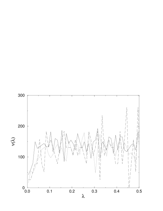
Figure 4.13: The spectral densities obtained at $\beta=6.0,\ 6.2,\ 6.4$ after 23 (solid), 46 (dotted) and 80 (dashed) cooling sweeps respectively.

4.2 Discussion

One qualitative feature that is common to all the instanton ensembles that we have investigated, is that they lead to spontaneous chiral symmetry breaking. A second, and striking, qualitative feature is that the spectral density diverges as $\lambda\to 0$. The divergence follows an approximate power law, $\propto\lambda^{-d}$, where $d$ decreases as the density of the instantons increases. Moreover we have seen that it is possible to have a stronger divergence for denser gases if one has a sufficient range of instanton sizes, of the kind that one finds in the lattice instanton ensembles. We have also tried to fit the divergence with a logarithmic form, since this is what one expects in leading-order quenched chiral perturbation theory [38, 39, 40]. (It has also been seen by unfolding the microscopic spectral density obtained via Random Matrix Theory [34, 35, 36, 37].) However such logarithmic fits are usually unacceptable, and where they are not it is a trivial consequence of the power exponent $d$ being small, as in equation (3.6). It is interesting to note that if one attempts to sum the leading-logs of quenched chiral perturbation theory, one can obtain [41, 42] a power divergence. The exponent of this divergence is $d=\delta/(1+\delta)$ where the parameter $\delta$ is simply related to the elementary pseudoscalar flavour singlet annihilation diagram (whose iteration provides an estimate of the mass of the $\eta^{\prime}$ in full QCD). The strength of this diagram is related, in turn, to the topological structure of the quenched vacuum [8, 9, 10], and so this suggests an approach to constructing a detailed link between our approach and that of chiral perturbation theory. It is amusing to note that the most recent quenched QCD estimates [22, 20] of $\delta$, obtained from chiral extrapolations where this parameter multiplies the quenched chiral log term, suggest a value $\delta\sim 0.1$ which is consistent with the kind of weak divergence we typically observe on the cooled instanton ensembles (see Table 4.1).

We have furthermore found evidence, from a comparison of the Dirac spectral densities, for some of the claims in [48]: in particular for the screening of topological charges in the quenched QCD vacuum, for the smallness of finite volume corrections and for the claim that if the number of cooling sweeps is varied with $\beta$ so that the number of topological charges per unit physical volume is constant, then the physical observables show scaling.

However we have also found that fermionic physical observables, such as the chiral condensate, vary strongly with the number of cooling sweeps. This contradicts the expectation that a moderate amount of cooling should only eliminate short distance fluctuations and so should not alter the physically important small-$\lambda$ end of the spectral density. Whether this is a problem with cooling per se or whether, as one would expect, it indicates the increasing unreliability of the instanton “pattern recognition” algorithms of [48] as one decreases the number of cooling sweeps, is a question we are not able to address. The resulting uncertainty is particularly important for the significance of the small-$\lambda$ divergence. We have seen that this divergence ranges from being strong to being negligible depending on which of the lattice instanton ensembles is used. It is strong for the larger number of cooling sweeps, which is where the instanton pattern recognition should be more reliable. On the other hand, a recent analysis [52] suggests that it is the instanton ensembles obtained with less cooling, where the low-$\lambda$ peaking is negligible, that are the more physical. So although we do find that instantons generically produce a divergence in the chiral condensate of quenched QCD, it is not clear whether it is strong enough to have any impact on the predictions for physical quark masses. One lesson is unambiguous: there is more that needs to be done before one can claim to have completely understood the true instanton structure of the gauge theory vacuum.

Set	$\beta$	$L^{3}T$	a(fm)	Cools	$N_{c}$	$\overline{N}_{T}/V$ ($fm^{-4}$)	f
A	6.0	$16^{3}48$	0.098	23	100	9.1	4.2
B	6.0	$16^{3}48$	0.098	46	100	3.2	1.9
C	6.0	$32^{3}64$	0.098	46	50	3.5	2.84
D	$6.0_{RP}$	$32^{3}64$	0.098	46	50	3.5	2.84
E	$6.0_{SS}$	$32^{3}64$	0.098	46	50	3.5	1.85
F	$6.0_{\rho>0.12}$	$32^{3}64$	0.098	46	50	3.1	2.82
G	6.2	$24^{3}48$	0.072	46	100	8.9	4.9
H	6.4	$32^{3}64$	0.0545	30	20	56.6	12.4
I	6.4	$32^{3}64$	0.0545	50	20	21.7	8.5
J	6.4	$32^{3}64$	0.0545	80	20	9.2	5.3

Table 4.1: Some information about the data analysed in this chapter. $V$ is the total spacetime volume, $\overline{V}_{I}$ is the average volume of an object in the ensemble, $\overline{N}_{T}$ is the average number of topological charges per configuration and $N_{c}$ is the number of configurations in the ensemble. The subscript RP stands for random positioning of objects whilst SS stands for all the objects being set to the same size. Power law fits of the data were possible (had reasonable statistical and systematic errors) for sets C, D and E, and had degree of divergence $d=0.251\pm 0.069,\ 0.585\pm 0.047$ and $0.186\pm 0.060$ with $\chi^{2}/N_{DF}=1.6,\ 2.2$ and 2.4 respectively.

Chapter 5 Unquenched QCD ensemble

In chapter 3 we carried out simulations on random configurations. We then proceeded in chapter 4 to study instanton ensembles derived from gauge configurations generated with the correct gauge weighting. In the spirit of Dædalus (whilst recalling the misfortune of his child) we turn now to simulations carried out on ensembles of instantons which incorporate both a gauge weighting and a fermion weighting. The results presented in this chapter have been published elsewhere [32].

One possible method for doing so would be to follow the equivalent path to the previous chapter, but, based on dynamical fermion ensembles. This is however not possible currently as there is only limited data available on the topological content of the full QCD vacuum (that is to say, the decomposition 2.1 has yet to be carried out in a detailed and systematic way for a variety of volumes, lattice spacings, pattern recognition algorithms etc.). We therefore revert to the method of chapter 3 and generate synthetic configurations. How do we incorporate the correct weightings into our model ?

5.1 Ensemble generation

5.1.1 The gauge weighting

We use a Poisson distribution for the gauge weighting for the number of instantons and anti-instantons in any configuration. The two distributions are independent so the joint distribution is simply the product of Poisson distributions:

$$P(N_{A}=s,N_{I}=t)=\exp(-2\mu)\frac{\mu^{s+t}}{s!t!}$$ (5.1)

where $\mu$ is the mean number of instantons (as well as anti-instantons) in the gas if we used the gauge weighting alone. This is analogous to equation 3.12 with $\mu=N_{T}/2$. (The variance is a factor of 2 greater using the Poisson weighting but such numerical factors should be unimportant.)

5.1.2 The fermion weighting

We claim that we are generating the low lying eigenvalue spectrum of the Dirac operator for any given instanton configuration. It is therefore easy to give the fermion weighting as the determinant for the configuration:

$$\det(\mbox{$i\!\!\not\!\!D$}[A]-im)\doteq(\overline{\lambda}_{NZ}^{2}+m^{2})^{(T-N_{A}-N_{I})/2}m^{|N_{A}-N_{I}|}\prod_{i=1}^{\min(N_{I},N_{A})}(\lambda_{i}^{2}+m^{2}),$$ (5.2)

where $\overline{\lambda}_{NZ}$ is a representative eigenvalue from mixing with/of non-zero modes, $T$ is the total number of modes of the Dirac operator and $\lambda_{i}$ are the eigenvalues generated for the configuration. The logic is as follows. Different configurations will contain different numbers of objects, and hence, direct comparison of determinants will not produce the correct weighting. The total number of eigenvalues is fixed, however, for a system with a fixed volume and ultra-violet cutoff. (Recall the lattice operator of dimension 786432 mentioned previously.) We think of the eigenvalues we generate as forming the crucial low lying spectrum; the remaining eigenvalues should be larger. We use a constant $\overline{\lambda}_{NZ}$ to represent these higher modes. It should be apparent that whilst the total number of modes $T$ appears in equation 5.2, it should not appear at all during the Monte Carlo simulation. This is because the Monte Carlo simulation requires only the ratio of determinants between old (accepted) configurations and new (trial) configurations, and hence, the constant $(\overline{\lambda}_{NZ}^{2}+m^{2})^{T/2}$ drops out. (It should also be noted that whilst we have written a factor of $(\overline{\lambda}_{NZ}^{2}+m^{2})^{1/2}$ for each non-zero mode, in the numerical code we used a factor $(\overline{\lambda}_{NZ}+m)$ instead. Given the qualitative nature of our definition of $\overline{\lambda}_{NZ}$ this is hopefully not a serious flaw.)

5.1.3 Monte Carlo simulation

To summarize, we can incorporate a reasonable gauge and fermion weighting into our model using only two paramters $\mu$ and $\overline{\lambda}_{NZ}$. The parameter $\mu$ is of course related to the packing fraction we desire for our configurations but does not determine it wholly. This is because the fermion determinant will also play a part in finding the equilibrium number of objects in the gas.

The Monte Carlo simulation begins with a random configuration. We then move a single object to generate a new trial configuration. This process is repeated as we “sweep” through the gas, moving each object in turn, accepting moves according to the standard Metropolis algorithm:

$$\begin{array}[]{lcll}P({\rm accept})&=&1&\det({\rm new})>\det({\rm old})\\ &=&\frac{\det({\rm new})}{\det({\rm old})}&{\rm otherwise}.\end{array}$$ (5.3)

We incorporate different numbers of flavours of fermions by raising the ratio to the power $N_{f}$. Periodically we attempt to either increase or decrease the number of instantons or anti-instantons by one (the period being every 10 attempted moves). We expect the system to come into equilibrium after some number of sweeps. As the change between successive configurations is small (differing only in the position of a single object or in having one extra or one fewer object), we normally require long separations to obtain independent configurations. Whilst we use all the configurations we generate (after leaving enough for the system to equilibriate), we ensure we have long runs to maximize the number of independent configurations.

5.1.4 Correlation functions

As we have a Monte Carlo simulation which moves objects around trying to generate configurations according to their overall weighting (both gauge and fermion), we can calculate correlation functions and use these to estimate particle masses ! We have two gluonic operators which we can use within our model, namely we have the topological charge density $Q$ and the number density of objects $N$ (which is our equivalent of the action density). How can we use these to calculate particle masses ?

$\langle Q(0)Q(t)\rangle$

We divide up our volume into a number of “strips” each of width $\delta t$. We can calculate the total charge in any strip simply by adding up the charges of all the objects contained within the strip. We call this $Q(t)$ for the strip $[t,t+\delta t)$. That is to say, $Q(t)=N_{I}(t)-N_{A}(t)$ where $N_{I/A}(t)$ are the number of instantons/anti-instantons contained with the strip. We can then work out the correlation function $\langle Q(0)Q(t)\rangle$ as a function of separation $t$.

$$\langle Q(0)Q(t)\rangle=\sum_{n}c_{n}\exp(-M_{n}t).$$ (5.4)

We can fit the resultant correlation function and attempt to extract the lowest mass (this will be the exponential which dies away slowest). Examination of the quantum numbers of the operator ($0^{-+}$, flavour singlet - as the operator is purely gluonic) reveals that this will be the mass within our model corresponding to the $\eta^{{}^{\prime}}$.

$\langle N(0)N(t)\rangle-\langle N(0)\rangle^{2}$

We can do the same as above but using our operator equivalent of the action. In this case $N(t)=N_{I}(t)+N_{A}(t)$. The only difference is that this time we have to subtract the constant vacuum expectation value, before fitting to an exponential. The mass we extract (if we can) will be the mass within our model corresponding to the $\sigma$ ($0^{++}$, flavour singlet).

Effective mass plots

As well as fitting exponentials to the correlation functions, we can plot the following quantity known as the effective mass:

$$m_{eff}(t)=-\ln\left(\frac{\langle{\cal O}(0){\cal O}(t)\rangle}{\langle{\cal O}(0){\cal O}(t-1)\rangle}\right),$$ (5.5)

where we have written our correlator with a generic operator ${\cal O}$ which can represent either the charge or the number density. It should be apparent that if the correlation function is in fact given by an exponential then our effective mass $m_{eff}(t)$ will be a straight line.

5.2 A few questions

There are a surprisingly large number of non-trivial questions we can ask within the framework of our model. Quantities of interest include:

• Spectral density. How does the spectral density behave with dynamical quarks ? Do we still get a power divergence as seen previously, $b(m)\lambda^{-d(m)}$ where $b(m),\ d(m)$ are now dependent upon the quark mass ? What is the behaviour of the spectral density as a function of the number of quark flavours $N_{f}$ ?

• Chiral condensate. What is the behaviour of $\langle\overline{\psi}\psi\rangle$(m) ? What is its behaviour as a function of the number of quark flavours ?

• Topological susceptibility. General arguments give the behaviour of this quantity as:

  $$\begin{array}[]{lcll}\langle Q^{2}\rangle(m)&\propto&mV&\chi SB\\ &\propto&m^{N_{f}}V&{\rm symmetric\ phase}.\end{array}$$ (5.6)

  Can our model reproduce such behaviour ?

• Particle masses. How do the masses of our versions of the $\sigma$ and $\eta^{{}^{\prime}}$ behave as functions of quark mass ? In reality, neither of these particles belongs to the octet of Goldstone bosons (in the chiral limit), hence, we wish for both particles to remain massive as we take the quark mass to zero. On a simpler level, can we even extract masses for such particles ?

We carry out simulations at $\overline{\lambda}_{NZ}=2$. This value is chosen because the mean eigenvalue for our “standard” quenched simulation with $f=1,\ V=1$ is approximately $1.12$. If we compare with figure 3.1 then it is apparent that this value is also far larger than the median eigenvalue (of the quenched ensemble). Whilst we do not know the “correct” value to use for $\overline{\lambda}_{NZ}$ (there is almost certainly no single correct value), $\approx 200\%$ of the quenched figure seems a reasonable place to start. As in the standard quenched simulation, we use $V=1$ with all objects of a fixed size $\rho=0.2$ (any objects which are inserted into the gas also have this size). The gauge weighting is given with $\mu=63$. Initially we have $N_{I}=63,\ N_{A}=63$, hence initially, the parameters are exactly those of the standard quenched simulation. We do not expect however for the system to find equilibrium with these values; once the fermion weighting is taken into account, the mean number of objects will undoubtedly be something else.

A difficulty with this approach lies with the concept of a replacement eigenvalue $\overline{\lambda}_{NZ}$. Our entire model is based around would-be zero modes and a replacement eigenvalue is admittedly, a very ad hoc method to incorporate other modes. We therefore also carry out unquenched simulations with a fixed total number of objects. The advantage of this is that we can have a fermion weighting given by the determinant without having to introduce a replacement eigenvalue at all. We still “sweep” through the configuration, moving objects as before, we still introduce and remove objects as before. The only difference is that every time we introduce an object, we remove an object of the opposite chirality, and, vice versa. The winding number can therefore only take even values but this is not a great loss considering that we have one fewer arbitrary parameter in our simulation.

We use a range of quark masses $m=0.15,\ 0.3$ and $0.5$ with $N_{f}=1,\ 2$ for both the case when we have a replacement eigenvalue and when we have the total number of objects fixed. In the latter case we also carry out simulations at some larger quark masses $m=1.0,\ 2.0$ and $3.0$. (It will turn out that there are technical and conceptual difficulties associated with running simulations for “large” quark masses when we have a replacement eigenvalue.) An ensemble consists of 630000 configurations. It should be noted however that the number of independent configurations is far smaller (perhaps two orders of magnitude smaller). We omit the first 63000 configurations (from data gathering) to allow the system to achieve equilibrium. (In truth a dynamic form of checking during the run would be preferable.)

5.3 Results

5.3.1 $N_{f}=1,\ \overline{\lambda}_{NZ}=2.0$.

We begin with one flavour of fermion with mass $m=0.5$. As a test of whether the system has achieved equilibrium, we plot the total number of objects in the gas $(N_{I}+N_{A})(c)$ as a function of the configuration number $c$ in figure 5.1.

Figure 5.1: $N_{f}=1,\ \overline{\lambda}_{NZ}=2.0,\ V=1,\ m=0.5$. The total number of objects as a function of the configuration number.

We see that the system oscillates around 70 objects in total (precise figures are given in table 5.1), radically different from the initial 126. We shouldn’t pay too much attention to the actual figure, for this will depend upon the value of $\overline{\lambda}_{NZ}$ we choose to use, the main importance is as a check of the algorithm and as a test of whether the system has come into equilibrium. We should also ensure that we are scanning net non-trivial topological sectors and are not stuck in the $Q=0$ sector. This can be seen in figure 5.2, which, is reassuring.

Figure 5.2: $N_{f}=1,\ \overline{\lambda}_{NZ}=2.0,\ V=1,\ m=0.5$. The net winding number as a function of the configuration number. We show only a section of the run for clarity.

What is the behaviour for lighter quark masses ? The lighter the quark, the greater the difficulty for simulation. This is because it becomes progressively more difficult to accept a trial configuration (e.g. consider a change from 63 objects of each chirality to 62 objects of each chirality; this requires us to go through a stage with 63 of one and 62 of the other - if we have massless objects then this will pose an insurmountable barrier as the determinant for the trial configuration will be precisely zero). The algorithm thus begins to “slow down” and its ergodicity gradually breaks down. We expect it to take longer to achieve equilibrium and longer to scan different sectors. Figures 5.3 and 5.4 which are the corresponding plots (to figures 5.1 and 5.2 respectively) are therefore pleasing; whilst there is undoubtedly some slowing down, there appears to be little difficulty with this range of quark masses.

Figure 5.3: $N_{f}=1,\ \overline{\lambda}_{NZ}=2.0,\ V=1,\ m=0.15$. The total number of objects as a function of the configuration number.

Reassured that the algorithm is behaving, we move onto the spectral density. Figure 5.5 shows the spectral density for the three quark masses. The first thing to note is that the spectral density appears to diverge as $\lambda\rightarrow 0$ for all three masses.

Figure 5.4: $N_{f}=1,\ \overline{\lambda}_{NZ}=2.0,\ V=1,\ m=0.15$. The net winding number as a function of the configuration number. We show only a section of the run for clarity.

It is however, equally clear that the spectral density is not independent of the quark mass. This gives us hope that we may yet evade the Banks-Casher relation and achieve a finite quark condensate. Table 5.2 clearly shows that the coefficient of the divergence $b\rightarrow 0$ as $m\rightarrow 0$. Whilst this is not in itself enough to show that we will achieve a finite quark condensate, it is at least promising. In figure 5.6 we integrate these spectra and plot the corresponding quark condensate, a linear extrapolation shows that we obtain chiral symmetry breaking with a finite condensate.

Figure 5.5: $N_{f}=1,\ \overline{\lambda}_{NZ}=2.0,\ V=1$. The spectral density for quark mass $m=0.5$ (solid), 0.3 (long dashed) and 0.15 (dotted).

We can also verify that the ensembles we have generated possess the correct distribution of winding numbers (at least the first two moments have the correct behaviour !). This can be seen in table 5.1 and in figure 5.7. Whilst we expect to obtain a linear relationship for $\langle Q^{2}\rangle(m)$ even in the symmetric phase (for $N_{f}=1$), this is not a trivial test for our model.

Figure 5.6: The quark condensate $\langle\overline{\psi}\psi\rangle$ as a function of the quark mass $m$ from the spectra plotted in figure 5.5.

Figure 5.7: $N_{f}=1,\ \overline{\lambda}_{NZ}=2.0,\ V=1$. The second moment of the winding number distribution $\langle Q^{2}\rangle$ as a function of the quark mass $m$.

Our results seem to be suprisingly good considering the simplicity of the underlying model. We move onto an extreme test of the model, that of obtaining particle masses. Figure 5.8 shows the correlation function for the $\eta^{{}^{\prime}}$ and the $\sigma$ for $m=0.15$. We can see that the fermion weighting has set up highly non-trivial correlations amongst the objects. We consistently find the $\eta^{{}^{\prime}}$ channel to give a far cleaner signal than the $\sigma$ channel. A consequence of this is that we get far higher values for $\chi^{2}/N_{DF}$ for the exponential fit to the $\eta^{{}^{\prime}}$ data (see table 5.3). It should be stressed however that we have fitted the exponential to the entire range shown in figure 5.8. The maximum of this range $t=0.5$ corresponds to a separation half way around the torus i.e. the maximum possible separation involving only one co-ordinate. If we were concerned with the large $\chi^{2}/N_{DF}$ for this fit then we could certainly reduce the range and excise the region which is in theory the most useful, but in practice, mostly noise (e.g. $t\geq 0.3$). Coversely, the low $\chi^{2}/N_{DF}$ for the $\sigma$ is a consequence of the weakness of the signal, not the goodness of fit. Regardless of these reservations, this is still a remarkable result for our model, a fact underlined by the mass plot given in figure 5.9 which shows that both particles remain massive in the chiral limit.

Figure 5.8: $N_{f}=1,\ \overline{\lambda}_{NZ}=2.0,\ V=1$. Correlation functions for $\eta^{{}^{\prime}}\ (\star)$, and for $\sigma\ (\circ)$.

Figure 5.9: $N_{f}=1,\ \overline{\lambda}_{NZ}=2.0,\ V=1$. Particle masses. $\eta^{{}^{\prime}}$ ($\star$) and $\sigma$ ($\circ$) as a function of the quark mass.

Lastly, in figure 5.10, we give the effective mass plot corresponding to the $\eta^{{}^{\prime}}$ with $m=0.15$. This shows that whilst the particle masses we have given are plausible, we could easily pick a slightly different mass due to the noise in the data (even for the $\eta^{{}^{\prime}}$).

Figure 5.10: $N_{f}=1,\ \overline{\lambda}_{NZ}=2.0,\ V=1,\ m=0.15$. The effective mass for the $\eta^{{}^{\prime}}$ data shown in figure 5.8.

5.3.2 $N_{f}=2,\ \overline{\lambda}_{NZ}=2.0$.

The results we have found seem to indicate that we can obtain a large amount of (qualitative) information about QCD by focusing on simply instanton degrees of freedom. It is of course trivial to vary the number of fermion flavours, all that is required is to take the ratio of the determinants to the power $N_{f}$ in the Metropolis step. It should be apparent however that the algorithm will struggle even more as we reduce the quark mass, effectively our suppression is enhanced and it is even more difficult to accept trial configurations. This can be clearly seen in figure 5.11 where we show the total number of objects as function of the configuration number for a quark mass of $m=0.15$. This plot should be compared with figure 5.3 to see the degree of difficulty encountered by the algorithm. We are effectively becoming trapped in certain sectors, in order to sample the phase space as effectively as for the $N_{f}=1$ case, we would require even larger runs.

Figure 5.11: $N_{f}=2,\ \overline{\lambda}_{NZ}=2.0,\ V=1,\ m=0.15$. The total number of objects as a function of the configuration number.

This is only emphasised by figure 5.12 which shows the difficulty in moving between sectors of different net topological charge.

Figure 5.12: $N_{f}=2,\ \overline{\lambda}_{NZ}=2.0,\ V=1,\ m=0.15$. The net winding number as a function of the configuration number. We show only a section of the run for clarity.

We should therefore be a little sceptical of these results, it is not a question of being wrong, it is more a question of being incomplete - we have not sampled as much of the phase space as we would wish. It is however not all bad, we can see from these plots that we appear to have achieved equilibrium; we are oscillating around $N_{T}=60$, not far from the $N_{f}=1$ figure, as opposed to the initial $N_{T}=126$.

The spectral density for the three masses is depicted in figure 5.13. A quick comparison with figure 5.5 indicates that something very different is occuring for two flavours of fermions. Why is the spectral density so small in magnitude in comparison to the one flavour case ? It is evident that we are seeing chiral symmetry restoration; the eigenvalues have been pushed to larger values, and hence, the spectrum is greatly depleted at the crucial low eigenvalues. This can be seen explicitly by comparing the spectrums obtained at $m=0.15$ for $N_{f}=1$ and $N_{f}=2$, as shown in figure 5.14.

Figure 5.13: $N_{f}=2,\ \overline{\lambda}_{NZ}=2.0,\ V=1$. The spectral density for quark mass $m=0.5$ (solid), 0.3 (long dashed) and 0.15 (dotted).

Figure 5.14: $\overline{\lambda}_{NZ}=2.0,\ V=1,\ m=0.15$. A comparison of the spectral densities obtained for $N_{f}=1$ (dark-solid) and $N_{f}=2$ (light-dotted).

Whilst we would expect to get chiral symmetry restoration for a sufficiently high number of fermion flavours, we most certainly do not expect chiral symmetry restoration for $N_{f}=2$, this is, after all, the physical world to a good approximation ! We can see the problem graphically in figure 5.15 which shows the chiral condensate decreasing to zero with the quark mass. The fact that we get the correct quadratic behaviour of the topological susceptibility for chiral symmetry restoration, is, at best, small comfort (see figure 5.16).

Figure 5.15: The quark condensate $\langle\overline{\psi}\psi\rangle$ as a function of the quark mass $m$ from the spectra plotted in figure 5.13.

Figure 5.16: $N_{f}=2,\ \overline{\lambda}_{NZ}=2.0,\ V=1$. The second moment of the winding number distribution $\langle Q^{2}\rangle$ as a function of the quark mass $m$.

There are a number of possibilities as to where the difficulties lie. The first is that we are seeing a facet of the critical slowing down of our algorithm. In other words, it is possible that if we were to undertake longer runs which sample more of the phase space, or design a more efficient algorithm, then our results would be different. Whilst this is a possibility, it is one which we have not been able to test, mainly due to time constraints. A second (more likely) possibility, is that we are seeing results of finite size effects. Recall, we get chiral symmetry restoration if we take the quark mass to zero in a finite volume. But this is precisely what we have been doing ! (The tacit assumption being that we would have needed to go to smaller masses yet, if we were to see a similar effect for $N_{f}=1$.) If this is so, then instead of being a sign of the breakdown of our model, it will reaffirm that it seems to capture some essential properties of the underlying field theory. How can we test this possibility ? The easiest way would be to work with larger quark masses; if we are seeing finite size effects, then these should become less important for larger quark masses and we should recover the signal of symmetry breakdown.

There are a few problems with implementing this idea however. The first concerns the concept of a replacement eigenvalue. This should be larger than the eigenvalues from the would-be zero modes, preferably far larger than the median such eigenvalue. This ensures that in the chiral limit, the main contribution to the spectral density is from the would-be zero modes (hence we concentrate upon them). When we are working with larger quark masses, our model is still based around the would-be zero modes. However, the contribution to the spectral density is no longer given mainly by the would-be zero modes (as all the eigenvalues are in fact shifted $\lambda\rightarrow(\lambda^{2}+m^{2})^{1/2}$), and the non-zero modes also contribute. A second problem is of a more practical nature. It lies with the fact that the number of objects is a dynamical quantity, furthermore, it is a dynamical quantity which depends upon the quark mass. Table 5.1 shows that we get fewer objects as we increase the quark mass, we have only $\approx 21$ objects of each chirality per configuration for $N_{f}=2,\ m=0.5$. What is happening is that the gas is becoming increasing dilute, for larger quark masses we get increasingly trivial configurations containing very few objects. (This is especially a problem as we are using hard sphere wavefunctions so it is easy to get accidental zero eigenvalues and, hence, zero determinants.) We therefore move to the second type of ensemble. In this case we fix the total number of objects as described previously. This alleviates both the conceptual, and, the practical problem, and, allows us to probe whether the restoration of chiral symmetry which we are seeing is a finite size effect, or, whether we face a breakdown of our model.

5.3.3 $N_{f}=1,2$. Fixed $N_{T}$.

Tables 5.1, 5.2 and 5.3 indicate that we get the same qualitative behaviour as before for $m=0.15,\ 0.3$ and $m=0.5$ for both $N_{f}=1$ and $N_{f}=2$. In figure 5.17 we plot the spectral density for $N_{f}=1$ for these quark masses. We see as in the cases where we varied $N_{T}$, a divergent spectral density (see figure 5.5). We plot the quark condensate corresponding to these spectra in figure 5.18, and we see, as in figure 5.6, chiral symmetry breakdown with a finite quark condensate.

Figure 5.17: $N_{f}=1$, Fixed $N_{T},\ V=1$. The spectral density for quark mass $m=0.5$ (solid), 0.3 (long dashed) and 0.15 (dotted).

Figure 5.18: $N_{f}=1$, Fixed $N_{T},\ V=1$. The quark condensate $\langle\overline{\psi}\psi\rangle$ as a function of the quark mass $m$.

So, for $N_{f}=1$ we get the behaviour we would expect. We study the more interesting $N_{f}=2$ case in more detail, and, in particular we simulate at higher quark masses.

Figure 5.19: $N_{f}=2$, Fixed $N_{T},\ V=1$. The spectral density for quark mass $m=0.15$ (solid) and $m=3.0$ (long dashed).

Figure 5.19 show the spectra we obtain for $m=0.15$ and $m=3.0$ respectively. We can immediately see the difference between the two; the spectra corresponding to the smaller mass shows the depletion of eigenvalues at small $\lambda$ that we expect to see if chiral symmetry is to be restored (compare with figure 5.14); the spectra corresponding to $m=3.0$ shows no such depletion.

Figure 5.20: $N_{f}=2$, Fixed $N_{T},\ V=1$. The quark condensate $\langle\overline{\psi}\psi\rangle$ as a function of the quark mass $m$.

If we integrate the spectra for the various masses then we get figure 5.20. This is a wonderful figure for us, it is precisely what we had hoped to see. We see at the larger quark masses the sure sign of chiral symmetry breakdown; as we move from $m=3.0$ to $m=1.0$, the quark condensate increases, and, a linear extrapolation leads to a finite non-zero condensate. As we reduce the mass further however, we get a totally different behaviour, the quark condensate collapses towards zero, behaviour consistent with the trivial restoration of chiral symmetry due to finite volume effects. The corresponding plot of $\langle Q^{2}(m)\rangle$ given in figure 5.21 is also pleasing, we see approximately linear behaviour for the larger quark masses, as we would expect for chiral symmetry breakdown, and, approximately quadratic behaviour for the smaller quark masses as before (see 5.16).

Figure 5.21: $N_{f}=2$, Fixed $N_{T},\ V=1$. The second moment of the winding number distribution $\langle Q^{2}\rangle$ as a function of the quark mass $m$.

We even find the behaviour of the $\eta^{{}^{\prime}}$ mass to be as before, it is massive in the chiral limit (see table 5.3). We cannot extract masses so easily for the $\sigma$ as this relies on correlations of the number of objects in slices through our spacetime, and, we have now fixed the total number of objects in every configuration.

5.4 Discussion

We have managed to extract a large amount of physics from our model. Important results include the fact that we expect a spectral density which is divergent at finite quark mass even in full QCD. The parameters of the divergence are mass dependent however, and, we obtain a finite quark condensate, as we must. We find that chiral symmetry is broken for $N_{f}=1$ but restored for $N_{f}=2$. We have strong evidence however, that the restoration is due to finite volume effects, and, that chiral symmetry is broken within the framework of our model, even for the $N_{f}=2$ case. Our model further agrees with predictions of the form for the winding number distribution as a function of quark mass, both for when chiral symmetry is broken, and, when it is restored. This is highly non-trivial and most unexpected. The presence of the fermion determinant generates non-trivial correlations between objects. Interpreting these correlations in terms of particles, we obtain masses for the $\eta^{{}^{\prime}}$ and the $\sigma$ which remain massive in the chiral limit.

Set	$\overline{\lambda}_{NZ}$	$N_{f}$	$m$	$\langle Q\rangle$	$\langle Q^{2}\rangle$	$\langle N_{I}\rangle$
A	2.0	1	0.5	0.152	25.65$\pm$0.45	35.53
B	2.0	1	0.3	-0.078	14.28$\pm$0.16	34.91
C	2.0	1	0.15	-0.209	8.13$\pm$0.04	35.75
D	2.0	2	0.5	-0.014	5.04$\pm$0.04	21.35
E	2.0	2	0.3	-0.059	2.43$\pm$0.03	23.17
F	2.0	2	0.15	-0.016	0.72$\pm$0.01	30.85
G	-	1	3.0	-0.403	98.615$\pm$0.78	62.80
H	-	1	2.0	0.061	80.097$\pm$0.92	63.03
I	-	1	1.0	-0.111	60.383$\pm$0.49	62.95
J	-	1	0.5	-0.046	34.22$\pm$0.26	62.98
K	-	1	0.3	-0.015	22.00$\pm$0.19	62.99
L	-	1	0.15	0.027	11.66$\pm$0.07	63.01
M	-	2	3.0	0.139	83.20$\pm$0.64	63.07
N	-	2	2.0	-0.193	62.49$\pm$0.40	62.90
O	-	2	1.0	-0.147	31.37$\pm$0.13	62.93
P	-	2	0.5	-0.033	11.61$\pm$0.10	62.98
Q	-	2	0.3	-0.089	4.71$\pm$0.05	62.96
R	-	2	0.15	-0.043	0.89$\pm$0.02	62.98

Table 5.1: Some information about the synthetic ensembles analysed in this chapter. A “-” indicates that the parameter is inapplicable, in this case, the sets are with fixed $N_{T}$ and hence, do not require a replacement eigenvalue $\overline{\lambda}_{NZ}$.

Set	b	d	$\chi^{2}/N_{DF}$
A	2.904$\pm$0.158	0.668$\pm$0.008	1.09
B	1.956$\pm$0.181	0.699$\pm$0.017	0.94
C	0.491$\pm$0.058	0.861$\pm$0.022	2.41
D	0.228$\pm$0.031	0.882$\pm$0.021	1.15
E	0.043$\pm$0.009	0.979$\pm$0.032	1.44
F	-	-	-
G	30.917$\pm$3.324	0.300$\pm$0.018	0.99
H	28.766$\pm$2.058	0.307$\pm$0.013	1.35
I	36.517$\pm$4.636	0.252$\pm$0.019	1.41
J	24.048$\pm$2.936	0.288$\pm$0.019	2.05
K	17.599$\pm$2.632	0.309$\pm$0.023	3.27
L	4.395$\pm$0.586	0.478$\pm$0.024	4.20
M	30.410$\pm$3.919	0.296$\pm$0.020	1.17
N	30.990$\pm$2.520	0.285$\pm$0.014	1.57
O	17.665$\pm$1.714	0.343$\pm$0.017	1.41
P	4.404$\pm$0.267	0.519$\pm$0.013	1.99
Q	0.580$\pm$0.051	0.788$\pm$0.019	1.55
R	0.006$\pm$0.002	1.307$\pm$0.043	2.30

Table 5.2: The spectral densities for the ensembles given in table 5.1. A “-” indicates that a satisfactory fit was not possible.

Set	$\eta^{{}^{\prime}}$	$\chi_{\eta^{{}^{\prime}}}^{2}/N_{DF}$	$\sigma$	$\chi_{\sigma}^{2}/N_{DF}$
A	11.180$\pm$0.466	10.6	11.589$\pm$2.612	0.566
B	11.880$\pm$0.600	14.61	11.083$\pm$3.149	0.229
C	12.271$\pm$0.548	15.00	9.426$\pm$2.673	1.44
D	18.849$\pm$0.775	5.94	14.691$\pm$3.589	0.640
E	18.904$\pm$0.892	8.01	19.011$\pm$3.291	0.708
F	19.265$\pm$0.873	8.75	29.955$\pm$3.592	5.899
G	9.503$\pm$2.328	0.55	-	-
H	6.618$\pm$0.908	2.10	-	-
I	11.147$\pm$0.490	4.59	-	-
J	11.313$\pm$0.589	12.40	-	-
K	10.969$\pm$0.278	14.51	-	-
L	11.620$\pm$0.290	16.44	-	-
M	11.895$\pm$1.275	1.524	-	-
N	12.642$\pm$0.951	3.405	-	-
O	13.780$\pm$0.454	7.900	-	-
P	15.190$\pm$0.465	11.17	-	-
Q	15.884$\pm$0.518	8.54	-	-
R	17.359$\pm$0.665	11.40	-	-

Table 5.3: Particle masses derived from ensembles given in table 5.1. $\chi_{\eta^{{}^{\prime}}}^{2}/N_{DF}$ refers to the chi-square of the exponential fit to the eta-correlation function, $\chi_{\sigma}^{2}/N_{DF}$ is the corresponding fit to the sigma-correlation function. A “-” indicates that a mass could not be extracted (see text).

Chapter 6 Conclusions

We established a framework which allowed us to construct a representation of the Dirac operator for a given configuration of instantons. The representation operated on the subspace of the Hilbert space spanned by the zero modes from the individual objects. We also approximated the Dirac operator by a simpler structure which we felt kept the bare essentials of the underlying theory. This has been a recurring idea throughout this work, to strip out as many details as possible whilst maintaining the symmetries and certain other properties of the underlying theory (the results in certain limits etc.).

It is currently not possible to carry out the simulations which could verify parts of this work. Some of the difficulties are conceptual (for instance, how can we disentangle instanton effects from other effects, such as the confinement mechanism, when we deal with the full field theory), others are practical (limitations of algorithms and computer power). However, we tested our model for “qualitative universality” and found this to hold: we get similar results regardless of the details of the type of wavefunction we used and the exact ansatz for the presence of the Dirac operator. A direct calculation on a lattice would be preferable, but our more limited checks at least satisfy the “necessary” requirement for making predictions for quenched and full QCD.

Whilst the approximations required to proceed with this work have effectively precluded quantitative predictions, we have been able to discern a number of qualitative features which are of interest. We have found strong evidence for chiral symmetry breaking. It seems that generic instanton configurations (which have no other dynamical effects at all - each configuration is random) are enough to break chiral symmetry. We have further seen that a divergence in the spectral density is almost ubiquitous for instanton gases. This leads to the prediction of a divergence in the chiral condensate in quenched QCD. We do not see such an effect from direct calculations of the Dirac spectra on lattice gauge configurations, presumably because the spectrum near $\lambda\rightarrow 0$ is distorted by lattice artefacts. We have found that the divergence can be parameterized for small $\lambda$ by a power law $\overline{\nu}(\lambda)=a+b\lambda^{-d}$. The power of the divergence $d$ is inversely related to the packing fraction of the gas, in particular the divergence is negligible for dense gases (though admittedly our methodology is doubtful in this limit). It is therefore possible, even in quenched QCD, for a dense gas of objects to break chiral symmetry and have a finite condensate. A detailed analysis found evidence that the divergence was not as a result of isolated barely overlapping dipoles of instanton and anti-instantons, but was in fact the result of complicated many body effects.

We found evidence of a “separation of scales” between large and small objects co-existing in a gas. A simple argument indicated that it was possible for the small objects in a gas to drive a divergent peak, even if they were overlapping with larger objects. This provides a mechanism whereby some of the successful phenomenological models, which require relatively low densities of objects (such as the instanton liquid model described in [4]) can be reconciled with lattice calculations indicating a far higher packing fraction [48]. We also found evidence for the screening of topological charge in the $SU(3)$ gauge theory, and, for scaling of spectra (if we altered the number of cools and $\beta$, the lattice coupling, in an appropriate fashion). An important “negative result” of our work is the conclusion that the Dirac spectrum for small $\lambda$ is strongly dependent upon the number of cooling sweeps undertaken to move from a “hot” lattice configuration to a collection of overlapping instantons. This leads to real ambiguities in the interpretation of the lattice data, how long should we cool for, should we extrapolate back to zero cools, etc. ? Some of these questions have been addressed in an interesting paper recently [52] but undoubtedly more work needs to be done in this area. This result is in marked contrast to the naïve hope that the spectral density, like for instance the topological susceptibility, would be relatively invariant to the local cooling process.

We have been able to generate ensembles of objects which incorporate both a gauge and a fermion weighting. These ensembles are our equivalent of full QCD instanton ensembles. We have found evidence that chiral symmetry is broken, and as before, we have a power law divergence for small $\lambda$. This would have been disastrous for our model (as we know QCD is a proper field theory and is certainly not pathological) if it wasn’t for the result that the divergence is quark mass dependent. In fact the spectra change in such a way that we obtain chiral symmetry breaking with a perfectly acceptable quark condensate. We believe this to be novel result which certainly merits further investigation. We found these results for both $N_{f}=1$ and $N_{f}=2$ (though we found strong evidence of finite size effects entering into our calculation for $N_{f}=2$ for our lowest quark masses). We found the correct behaviour for the topological susceptibility for both the broken phase (linear with respect to the quark mass), and, the symmetric phase (where restoration was due to finite size effects). Remarkably we have also been able to extract masses corresponding to the $\eta^{{}^{\prime}}$ and the $\sigma$. We have found both of these to be massive in the chiral limit.

Appendix A Calculation of overlap integrals.

A.1 Hard Sphere

The wavefunctions are given by:

$$\begin{array}[]{lcll}\langle x|\psi_{i}\rangle&=&1&\quad|x-x_{i}|\leq r_{i}\\ &=&0&\quad{\rm otherwise,}\end{array}$$ (A.1)

where $i=1,2$ labels the two objects in question. We wish to compute the integral:

$$\langle\psi_{1}|\psi_{2}\rangle=\int_{\mathbb{M}}\ d^{4}x\langle\psi_{1}|x\rangle\langle\psi_{2}|x\rangle,$$ (A.2)

where ${\mathbb{M}}$ is either ${\mathbb{T}}^{4}$ or ${\mathbb{R}}^{4}$. So we wish to calculate the volume of intersection of the two spheres. For simplicity, let us first consider the problem for ${\mathbb{R}}^{4}$. In this case we work out the separation $s$ of the objects in the usual Euclidean fashion. The two trivial cases are where $s>r_{1}+r_{2}$, in which case the intersection is zero, or where $s\leq|r_{1}-r_{2}|$, in which case one sphere is inside the other and the intersection is simply the volume of the smaller $(\pi^{2}/2)\min(r_{1},r_{2})^{4}$.

Figure A.1: Intersection of two spheres in ${\mathbb{R}}^{4}$.

The non-trivial case $|r_{1}-r_{2}|<s\leq r_{1}+r_{2}$ is depicted in figure A.1 and its evaluation is a simple excercise in geometry. It consists of adding up the volumes $A$ and $B$. We will calculate the volume of $A$, as the calculation of $B$ is similar. The angle $\theta$ as shown in figure A.1 is given by:

$$\cos\theta=\frac{s^{2}+r_{2}^{2}-r_{1}^{2}}{2r_{2}s}\ .$$ (A.3)

We first calculate the volume of the cone which originates at $x_{2}$:

$$\int_{0}^{r_{2}}dr\int_{0}^{2\pi}d\phi\int_{0}^{\theta}d\theta_{2}\int_{0}^{\pi}d\theta_{1}r^{3}\sin^{2}\theta_{2}\sin\theta_{1}=\frac{r_{2}^{4}\pi}{2}\left(\theta-\frac{sin(2\theta)}{2}\right)$$ (A.4)

The volume $A$ is given by A.4 take away the volume of the right-angled cone which originates at $x_{2}$. The volume of the right-angled cone is simply $(\pi/3)r_{2}^{4}\cos\theta\sin^{3}\theta$. Therefore:

$$Vol.(A) = V(\theta)$$ (A.5)

$$= \frac{r_{2}^{4}\pi}{2}\left(\theta-\sin 2\theta\left(\frac{1}{2}+\frac{1}{3}\sin^{2}\theta\right)\right)$$

The volume of our intersection is given by $V(\theta)+V(\omega)$, where $\omega$ is defined analogously to $\theta$.

The overlap when the space is ${\mathbb{T}}^{4}$ is only slightly more complicated. In this work all objects obey the condition $r_{i}<l/2\ \forall i$, where $l$ is the length of the side of the periodic box. This simplifies matters considerably (and also make sense from a physics viewpoint as otherwise we would be almost certain to be suffering from finite size effects). A little thought will confirm that the following algorithm works for the case of the periodic box (for simplicity consider the unit periodic box - the generalisation is obvious).

Consider the overlap of two objects, A and B in a periodic box. Do nothing with object A. Consider the set of 81 objects $B_{S},\ S=1,\ldots,81$ given by translating object B to all unit boxes adjacent to the original i.e. $x_{B}\rightarrow x_{B}+v$ where the components of the shift vector $v^{i}\in\{-1,0,1\}$. The overlap integral is given by

$$\langle\psi_{A}|\psi_{B}\rangle=\sum_{S=1}^{81}Vol.(A\cap B_{S}),$$ (A.6)

where the volume of intersection is calculated in ${\mathbb{R}}^{4}$ as above.

A.2 Gaussian

We wish to construct a smooth function which is periodic with period the unit box (again for simplicity). We do so by first defining:

$$G(x;x_{j}^{\pm},\sigma_{j}^{\pm},l) = \frac{1}{\sqrt{2\pi}\sigma_{j}^{\pm}}\exp\left(\frac{-(x-x_{j}^{\pm}-l)^{2}}{2\sigma_{j}^{\pm 2}}\right).$$ (A.7)

where $x_{j}^{\pm}$ lies in the unit four box with $l\in{\mathbb{Z}}^{4}$. The Gaussian zero mode wavefunction is given by:

$$\langle x|\psi_{j}^{\pm}\rangle = N\sum_{l\in{\mathbb{Z}}^{4}}G(x;x_{j}^{\pm},\sigma_{j}^{\pm},l),$$ (A.8)

where $N$ is a suitable normalization constant. If we now wish to integrate this function on ${\mathbb{T}}^{4}$ then all we do is integrate over the unit box. It is relatively simple to perform this integral, the results being:

$$\int_{{\mathbb{T}}^{4}}d^{4}xG(x;x_{1},\sigma_{1})G(x;x_{2},\sigma_{2})=\frac{1}{2\pi^{2}(\sigma_{1}^{2}+\sigma_{2}^{2})}\sum_{m_{\mu}\in{\mathbb{Z}}}\exp\left(\frac{(x_{1}-x_{2}+m)^{2}}{2(\sigma_{1}^{2}+\sigma_{2}^{2})}\right)$$ (A.9)

This is an infinite series which does not have an obvious analytical solution (though it certainly converges). In practice we truncate the series after some number of terms, we have found for $\sigma\leq 0.2$ that $m_{\mu}\in\{-1,0,1\}$ leads to negligible errors.

A.3 Classical zero mode

This wavefunction is defined by:

$$\langle x|\psi_{i}\rangle=\frac{\sqrt{2}}{\pi}\frac{\rho_{i}}{(\rho_{i}^{2}+(x-x_{i})^{2})^{3/2}}$$ (A.10)

We wish to evaluate the inner product of two such functions over ${\mathbb{R}}^{4}$. This can be done by the standard method of Feynman parameters to yield the following integral solution:

$$\langle\psi_{i}\psi_{j}\rangle=\frac{8}{\pi}\frac{\rho_{i}}{\rho_{j}}\int_{0}^{1}dq\frac{\sqrt{q(1-q)}}{1+q(\frac{s^{2}}{\rho_{j}^{2}}+\frac{\rho_{i}^{2}}{\rho_{j}^{2}})-q^{2}\frac{s^{2}}{\rho_{j}^{2}}}.$$ (A.11)

The lack of a closed form expression for this overlaps makes the calculation far slower than when we use the hard sphere (or even the Gaussian) wavefunction. One can indeed evaluate this integral in terms of the hypergeometric function of two variables, but the quickest way of evaluating this function is to calculate the above integral !

Appendix B Error estimation & Best Fits

B.1 Error estimation

All errors quoted in this work have been calculated using “jack-knife” methodology. This is similar to conventional methods except more robust when data is limited (as for instance in the case of configurations of instantons derived from lattice data). The idea is as follows:

• Split up the data into $N$ sets $d_{1},\ldots,d_{N}$, each of which containts $(N-1)/N$ of all the data.

• Calculate $N$ estimates of the desired quantity $\Phi_{1},\ldots,\Phi_{N}$, where $\Phi_{i}$ uses the data from $d_{i}$. So for instance, consider the case of $N=10$ and the example of calculating the spectral density at a point $\lambda=\lambda_{0}$. In this case we would get $10$ estimates of the spectral density, each of which would use nine-tenths of the available data. The most important thing to note about these estimates is that they are not independent.

• An unbiased estimate of the mean is given by the usual formula:

  $$\hat{\mu}=\frac{1}{N}\sum_{i=1}^{N}\Phi_{i}$$ (B.1)

• An unbiased estimate of the variance is again given by the usual formula:

  $$\hat{s}^{2}=\frac{1}{N-1}\sum_{i=1}^{N}(\Phi_{i}-\hat{\mu})^{2}$$ (B.2)

• The distribution the mean is different however, the variance of the distribution is not given by $\hat{s}^{2}/N$ but by $N\hat{s}^{2}$. So the error estimate is given as:

  $$\hat{\mu}\pm N\hat{s}^{2}.$$ (B.3)

The advantage of this method is really in its robustness. If data is limited, for example, then the usual method of splitting data into $N$ sets each of which is independent and contains $1/N$ of the total data become unstable. (Consider the lattice data with 50 configurations in total: what sort of spectrum could we obtain is we used only 5 configurations as opposed to 45 ?)

B.2 Best Fits

We have a set of numerical data $\{x_{j},E(x_{j}),\sigma(x_{j})\}$ where $x_{j}$ denotes the points, $E(x_{j})$ denotes the values obtained and $\sigma(x_{j})$, the errors around those values. Consider a fit function $f(x;\alpha_{i})$ defined by a set of $K$ parameters $\{\alpha_{i},\ i=1,\ldots,K\}$. The “best fit” is given by finding the parameters $\{\alpha_{i}^{B}\}$ which minimize the $\chi^{2}$ of the fit:

$$\chi^{2}(\alpha_{1},\ldots,\alpha_{K})=\sum_{j=1}^{N}\frac{(f(x_{j};\alpha_{i})-E(x_{j}))^{2}}{\sigma_{j}^{2}}$$ (B.4)

There is no general procedure for finding these best parameters. When we are dealing with fit functions which are non-linear (in the parameters), such as the power law fit function 3.4, then the problem is not simple at all. Inevitably one uses a “canned package”, the one used in this thesis is the standard Levenberg-Marquardt method. These do not find the absolute minima of the $\chi^{2}$ function, they do find a minima, at least most of the time.

In practice, the quality of the data for the “synthetic” configurations is so high that the fitting program is robust. The situation is not so good for the lattice data. One way to test how good the fit is, is if one mutiplies all the $\sigma_{j}$ by a constant factor $\sigma_{j}\rightarrow c\sigma_{j}$. If one carries out the fit again, then the resultant parameters should be identical, only the $\chi^{2}$ should be altered, $\chi^{2}\rightarrow\chi^{2}/c^{2}$. This is always so for the synthetic data (to within hundreths of a percent), but not for the lattice data: the algorithm has wandered to a different minima in parameter space. These difficulties are to some extent inevitable if one is forced to use non-linear fits with limited data. We rely on comparisons with the synthetic data to give us confidence about our results for the lattice data.

Bibliography

- [1] S. Coleman, “The uses of instantons,” Aspects of Symmetry, 265-350, CUP (1985)
- [2] A.I. Vaǐnshteǐn, V.I. Zakharov, V.A. Novikov and M.A. Shifman, “Abc’s Of Instantons,” Sov. Phys. Usp. 24, 195 (1982).
- [3] D. Diakonov, “Chiral symmetry breaking by instantons,” Varenna Lectures 1995 hep-ph/9602375.
- [4] T. Schäfer and E.V. Shuryak, “Instantons in QCD,” Rev. Mod. Phys. 70, 323 (1998)
- [5] A.A. Belavin, A.M. Polyakov, A.S. Shvarts and Y.S. Tyupkin, “Pseudoparticle Solutions Of The Yang-Mills Equations,” Phys. Lett. 59B, 85 (1975).
- [6] R. Jackiw and C. Rebbi, “Vacuum Periodicity In A Yang-Mills Quantum Theory,” Phys. Rev. Lett. 37, 172 (1976).
- [7] C.G. Callan, R. Dashen and D.J. Gross, “Toward A Theory Of The Strong Interactions,” Phys. Rev. D17, 2717 (1978).
-
[8]
G. ’t Hooft, “Symmetry Breaking Through
Bell-Jackiw Anomalies,” Phys. Rev. Lett. 37, 8 (1976).
G. ’t Hooft, “Computation Of The Quantum Effects Due To A Four-Dimensional Pseudoparticle,” Phys. Rev. D14, 3432 (1976). - [9] E. Witten, “Current Algebra Theorems For The U(1) ’Goldstone Boson’,” Nucl. Phys. B156, 269 (1979).
- [10] G. Veneziano, “U(1) Without Instantons,” Nucl. Phys. B159, 213 (1979).
- [11] A.M. Polyakov, “Quark Confinement And Topology Of Gauge Groups,” Nucl. Phys. B120, 429 (1977).
- [12] D.G. Caldi, “Quark Mass Generation By Instantons,” Phys. Rev. Lett. 39, 121 (1977).
- [13] R.D. Carlitz and D.B. Creamer, “Light Quarks And Instantons,” Ann. Phys. 118, 429 (1979).
- [14] R. Jackiw and C. Rebbi, “Conformal Properties Of A Yang-Mills Pseudoparticle,” Phys. Rev. D14, 517 (1976).
- [15] R. Bott, Bull. Soc. Math. France 84, 251 (1956).
- [16] L.S. Brown, R.D. Carlitz and C. Lee, “Massless Excitations In Instanton Fields,” Phys. Rev. D16, 417 (1977).
- [17] S. Weinberg, “Anomalies,” The Quantum Theory of Fields Vol. II, 359-420, CUP (1996)
-
[18]
M.F. Atiyah and I.M. Singer, “The Index Of Elliptic
Operators. 1,” Annals Math. 87, 484 (1968).
M.F. Atiyah and I.M. Singer, “The Index Of Elliptic Operators. 3,” Annals Math. 87, 546 (1968). - [19] T. Banks and A. Casher, “Chiral Symmetry Breaking In Confining Theories,” Nucl. Phys. B169, 103 (1980).
- [20] S.R. Sharpe, “Progress in lattice gauge theory,” hep-lat/9811006.
- [21] R. Gupta, “Introduction to lattice QCD” hep-lat/9807028.
- [22] S. Aoki et al. [CP-PACS Collaboration], “Quenched light hadron spectrum,” hep-lat/9904012.
-
[23]
H.B. Nielsen and M. Ninomiya, “Absence Of Neutrinos
On A Lattice. 1. Proof By Homotopy Theory,” Nucl. Phys. B185,
20 (1981).
H.B. Nielsen and M. Ninomiya, “Absence Of Neutrinos On A Lattice. 2. Intuitive Topological Proof,” Nucl. Phys. B193, 173 (1981). - [24] G.R. Fleming et al., “The Domain wall fermion chiral condensate in quenched QCD,” Nucl. Phys. Proc. Suppl. 73, 207 (1999).
- [25] R. Mawhinney et al., “Quenched QCD with domain wall fermions,” Nucl. Phys. Proc. Suppl. 73, 204 (1999)
- [26] P. Chen et al., “Toward the chiral limit of QCD: Quenched and dynamical domain wall fermions,” hep-lat/9812011.
- [27] R.G. Edwards, U.M. Heller and R. Narayanan, “A study of chiral symmetry in quenched QCD using the overlap Dirac operator,” Phys. Rev. D59, 094510 (1999)
- [28] H. Neuberger, “Exactly massless quarks on the lattice,” Phys. Lett. B417, 141 (1998)
- [29] F. Niedermayer, “Exact chiral symmetry, topological charge and related topics,” Nucl. Phys. Proc. Suppl. 73, 105 (1999)
- [30] N. Dowrick and M. Teper, “Instantons, chiral symmetry breaking and the fate of the ultimate quenched calculation,” Nucl. Phys. Proc. Suppl. 42, 237 (1995).
- [31] U. Sharan and M. Teper, “Chiral symmetry breaking, instantons and the ultimate quenched calculation,” Nucl. Phys. Proc. Suppl. 73, 617 (1999)
- [32] U. Sharan and M. Teper, “Chiral symmetry breaking and instantons in both quenched and full QCD,” hep-ph/9910216.
- [33] E.V. Shuryak and J.J. Verbaarschot, “On baryon number violation and nonperturbative weak processes at SSC energies,” Phys. Rev. Lett. 68, 2576 (1992).
- [34] J.C. Osborn and J.J. Verbaarschot, “Thouless energy and correlations of QCD Dirac eigenvalues,” Nucl. Phys. B525, 738 (1998)
- [35] J.C. Osborn, D. Toublan and J.J. Verbaarschot, “From chiral random matrix theory to chiral perturbation theory,” Nucl. Phys. B540, 317 (1999)
- [36] J.J. Verbaarschot, private communication.
- [37] E.V. Shuryak, private communication.
- [38] S.R. Sharpe, “Lattice Calculations Of Electroweak Decay Amplitudes,” Nucl. Phys. Proc. Suppl. 17, 146 (1990).
- [39] C. Bernard and M. Golterman, “Chiral perturbation theory for the quenched approximation,” Nucl. Phys. Proc. Suppl. 26, 360 (1992).
- [40] M. Golterman, “Connections between lattice gauge theory and chiral perturbation theory,” hep-ph/9710468.
- [41] S.R. Sharpe, “Problems with the quenched approximation in the chiral limit,” Nucl. Phys. Proc. Suppl. 30, 213 (1993).
- [42] M. Golterman, private communication.
- [43] C. Michael and P.S. Spencer, “Cooling and the SU(2) instanton vacuum,” Phys. Rev. D52, 4691 (1995)
- [44] P. de Forcrand, M. Garcia Perez and I. Stamatescu, “Topology of the SU(2) vacuum: A Lattice study using improved cooling,” Nucl. Phys. B499, 409 (1997)
-
[45]
T. DeGrand, A. Hasenfratz and T.G. Kovacs,
“Topological structure in the SU(2) vacuum,” Nucl. Phys. B505,
417 (1997)
T. DeGrand, A. Hasenfratz and T.G. Kovacs, “Revealing topological structure in the SU(2) vacuum,” Nucl. Phys. B520, 301 (1998) - [46] P. de Forcrand, M. Garcia Perez, J.E. Hetrick and I. Stamatescu, “Topological properties of the QCD vacuum at T = O and T similar to T(c),” hep-lat/9802017.
- [47] A. Hasenfratz and C. Nieter, “Instanton content of the SU(3) vacuum,” Phys. Lett. B439, 366 (1998)
- [48] D.A. Smith and M.J. Teper [UKQCD Collaboration], “Topological structure of the SU(3) vacuum,” Phys. Rev. D58, 014505 (1998)
- [49] M.J. Teper, “Physics from the lattice: Glueballs in QCD: Topology: SU(N) for all N,” hep-lat/9711011.
- [50] S.J. Hands and M. Teper, “On The Value And Origin Of The Chiral Condensate In Quenched SU(2) Lattice Gauge Theory,” Nucl. Phys. B347, 819 (1990).
- [51] U. Sharan and M. Teper [UKQCD Collaboration], “On the spectral density from instantons in quenched QCD,” Phys. Rev. D60, 054501 (1999)
- [52] A. Ringwald and F. Schrempp, “Confronting instanton perturbation theory with QCD lattice results,” hep-lat/9903039.
- [53] A. Hart and M. Teper, work in progress.