Renormalization Group Invariant Matrix Elements of $\Delta S=2$ and $\Delta I=3/2$ Four-Fermion Operators without Quark Masses

Abstract

We introduce a new parameterization of four-fermion operator matrix elements which does not involve quark masses and thus allows a reduction of systematic uncertainties. In order to simplify the matching between lattice and continuum renormalization schemes, we express our results in terms of renormalization group invariant $B$-parameters which are renormalization-scheme and scale independent. As an application of our proposal, matrix elements of $\Delta I=3/2$ and SUSY $\Delta S=2$ operators have been computed. The calculations have been performed using the tree-level improved Clover lattice action at two different values of the strong coupling constant ($\beta=6/g^{2}=6.0$ and $6.2$), in the quenched approximation. Renormalization constants and mixing coefficients of lattice operators have been obtained non-perturbatively. Using lowest order $\chi$PT, we also obtain $\langle\pi\pi|O_{7}|K\rangle^{\mbox{\scriptsize NDR}}_{I=2}=(0.11\pm 0.02)$ GeV⁴ and $\langle\pi\pi|O_{8}|K\rangle^{\mbox{\scriptsize NDR}}_{I=2}=(0.51\pm 0.05)$ GeV⁴ at $\mu=2$ GeV.

BUHEP-99-23

FTUV/99-62

IFIC/99-65

ROME1-1265/99

PACS: 11.15.H, 12.38.G, 14.40.Aq and 12.15.Hh

1 Introduction

Since the original proposals of using lattice QCD to study hadronic weak decays [1]–[3], substantial theoretical and numerical progress has been made: the main theoretical aspects of the renormalization of composite four-fermion operators are fully understood [4, 5]; the calculation of $K^{0}$–$\bar{K}^{0}$ mixing, expressed in terms of the so-called renormalization group invariant $B$-parameter $\hat{B}_{K}$, has reached a level of accuracy which is unpaired by any other approach [6]–[9]; increasing precision has also been gained in the determination of the electro-weak penguin amplitudes necessary to the prediction of the CP-violation parameter $\epsilon^{\prime}/\epsilon$ [10]–[16]; attempts to compute the matrix element of the QCD penguin operator $O_{6}$ exist [17]. Finally, matrix elements of $\Delta S=2$ operators which are relevant to study FCNC effects in SUSY models have been also computed [16, 18].

Following the common lore, matrix elements of weak four-fermion operators are given in terms of the so-called $B$-parameters which measure the deviation of their values from those obtained in the Vacuum Saturation Approximation (VSA). A classical example is provided by the matrix element of the $\Delta S=2$ left-left operator $O^{\Delta S=2}=\bar{s}\gamma_{\mu}(1-\gamma_{5})d\;\bar{s}\gamma^{\mu}(1-\gamma_{5})d$ relevant to the prediction of the CP-violation parameter $\epsilon$

$$\langle\bar{K}^{0}|O^{\Delta S=2}|K^{0}\rangle=\frac{8}{3}M_{K}^{2}f_{K}^{2}B_{K}\ .$$ (1)

VSA values and $B$-parameters are also used for matrix elements of $\Delta S=1$ operators entering $\epsilon^{\prime}/\epsilon$, in particular $O_{6}=\bar{s}_{\alpha}\gamma_{\mu}(1-\gamma_{5})d_{\beta}\sum_{q}\bar{q}_{\beta}\gamma_{\mu}(1+\gamma_{5})q_{\alpha}$ and $O_{8}=3/2\bar{s}_{\alpha}\gamma_{\mu}(1-\gamma_{5})d_{\beta}\sum_{q}e_{q}\bar{q}_{\beta}\gamma_{\mu}(1+\gamma_{5})q_{\alpha}$ [19, 20]

$$\langle\pi\pi|O_{6}(\mu)|K\rangle_{I=0} = -4\left[\frac{M^{2}_{K}}{m_{s}(\mu)+m_{d}(\mu)}\right]^{2}(f_{K}-f_{\pi})\;B_{6}(\mu)\;,$$

$$\langle\pi\pi|O_{8}(\mu)|K\rangle_{I=2} = \sqrt{2}f_{\pi}\left[\left(\frac{M^{2}_{K}}{m_{s}(\mu)+m_{d}(\mu)}\right)^{2}\right.$$ (2)

$$- \left.\frac{1}{6}\left(M_{K}^{2}-M_{\pi}^{2}\right)\right]\;B^{(3/2)}_{8}(\mu)\;.$$

Contrary to $\langle\bar{K}^{0}|O^{\Delta S=2}|K^{0}\rangle$ and $\langle\pi\pi|O_{6}|K\rangle_{I=0}$ which vanish in the chiral limit, the matrix element of the left-right operator $\langle\pi\pi|O_{8}|K\rangle_{I=2}$ remains finite. For this reason, the dependence of this amplitude on quark masses is expected to be smooth because it only enters in higher orders of the chiral expansion

$$\left(\frac{M^{2}_{K}}{m_{s}+m_{d}}\right)^{2}\sim C_{1}+C_{2}\;(m_{s}+m_{d})+{\cal O}(m_{s}^{2})\,,$$ (3)

where $C_{1,2}$ are constants, independent of quark masses.

Quark masses, however, appear explicitly in (1). Since in the VSA (and in the $1/N$ expansion [21]) the expression of the matrix elements is quadratic in $m_{s}+m_{d}$, predictions for the physical amplitudes are heavily affected by the specific value taken for this quantity. Contrary to $f_{K}$, $M_{K}$, etc., quark masses are not directly measured by experiments and the present accuracy in their determination is still rather poor [22]. Therefore, the “conventional” parameterization (1) introduces a large systematic uncertainty in the prediction of the physical amplitudes of $\langle O_{6}\rangle_{I=0}$ and $\langle O_{8}\rangle_{I=2}$ (and of any other left-right operator). Moreover, whereas for $O^{\Delta S=2}$ we introduce $\hat{B}_{K}$ as an alias of the matrix element, by using (1) we replace each of the matrix elements with 2 unknown quantities, i.e. the $B$-parameter and $m_{s}+m_{d}$. Finally, in many phenomenological analyses, the values of the $B$-parameters of $\langle O_{6}\rangle_{I=0}$ and $\langle O_{8}\rangle_{I=2}$ and of the quark masses are taken by independent lattice calculations, thus increasing the spread of the theoretical predictions . All this can be avoided in the lattice approach, where matrix elements can be computed from first principles.

In this paper, we propose a new parameterization of matrix elements in terms of well known experimental quantities, without any reference to the VSA and therefore to the strange (down) quark mass. This results in a determination of physical amplitudes with smaller systematic errors. As an application of our proposal we have reanalyzed the lattice correlation functions considered in [16] to estimate matrix elements of $\Delta I=3/2$ operators and of the operators of the most general $\Delta S=2$ Hamiltonian. By comparing the results of the present study with those of ref. [16] we show all the advantages of the new parameterization. We give the results for operators renormalized non-perturbatively in the RI (MOM) scheme [14, 16, 23, 24].

We also introduce a Renormalization Group Invariant (RGI) definition of matrix elements (and Wilson coefficients). This definition generalizes to an arbitrary basis a concept which has been adopted very successfully for the $K^{0}$–$\bar{K}^{0}$ mixing amplitude, which is usually written in terms of the RGI $B$-parameter, $\hat{B}_{K}$. With our definition, Wilson coefficients and operators are renormalization-scale and scheme independent. This will hopefully avoid some confusion existing in the literature. This confusion is generated by the fact that (perturbative) Wilson coefficients and (non-perturbative) matrix elements have been computed using different techniques, regularizations, renormalization schemes (different versions of NDR and HV, DRED, RI-MOM with different external states) and renormalization scales. In this way, the effective Hamiltonian is splitted in terms which are individually scheme and scale independent.

The remainder of the paper is organized as follows: in sec. 2 we define operators and matrix elements considered in the present study and introduce the new parameterization of the matrix elements; in sec. 3 we give the RGI definition for a generic operator basis; in sec. 4 we present our new numerical results and compare them with those obtained with the “conventional” definition of the $B$-parameters; in sec. 5 we give our best estimates of the matrix elements and in sec. 6 we present our conclusions. All details concerning the non-perturbative renormalization of lattice operators and the extraction of matrix elements from correlation functions are not discussed here since they can be found in refs. [14, 16]. In particular, in ref. [16], the same set of lattice data was analyzed. We compare the results of the present study to those of this reference.

2 Matrix elements without quark masses

In this section we introduce the notation and define operators and matrix elements used in this paper. The new parameterization, that does not involve any reference to quark masses, is defined here. An alternative parameterization which (for reasons explained below) has not been used in our numerical analysis, but may be useful in the future, is also considered in this section.

• $\Delta S=2$ operators:
  The analysis of $K^{0}-\bar{K}^{0}$ mixing with the most general $\Delta S=2$ effective Hamiltonian requires the knowledge of the matrix elements $\langle\bar{K}^{0}|O_{i}|K^{0}\rangle$ of the following operators [25]–[27]

  $$O_{1} = \bar{s}^{\alpha}\gamma_{\mu}(1-\gamma_{5})d^{\alpha}\ \bar{s}^{\beta}\gamma_{\mu}(1-\gamma_{5})d^{\beta},$$

  $$O_{2} = \bar{s}^{\alpha}(1-\gamma_{5})d^{\alpha}\ \bar{s}^{\beta}(1-\gamma_{5})d^{\beta},$$

  $$O_{3} = \bar{s}^{\alpha}(1-\gamma_{5})d^{\beta}\ \bar{s}^{\beta}(1-\gamma_{5})d^{\alpha},$$ (4)

  $$O_{4} = \bar{s}^{\alpha}(1-\gamma_{5})d^{\alpha}\ \bar{s}^{\beta}(1+\gamma_{5})d^{\beta},$$

  $$O_{5} = \bar{s}^{\alpha}(1-\gamma_{5})d^{\beta}\ \bar{s}^{\beta}(1+\gamma_{5})d^{\alpha},$$

  where $\alpha$ and $\beta$ are color indices and $O^{\Delta S=2}\equiv O_{1}$. For $\langle\bar{K}^{0}|O_{i}|K^{0}\rangle$, only the parity-even parts of the operators of eqs. (4) contribute. $\langle\bar{K}^{0}|O_{1}|K^{0}\rangle$ is expected to vanish in the chiral limit, whereas the matrix elements $\langle\bar{K}^{0}|O_{i}|K^{0}\rangle$ ($i=2,3,4,5$) remain finite. For the latter, close to the chiral limit, we expect a mild dependence on the quark masses, as given in eq. (3).

  Omitting terms which are of higher order in Chiral perturbation theory ($\chi$PT), the $B$-parameters are usually introduced using the expressions [16]

  $$\langle\bar{K}^{0}|O_{1}(\mu)|K^{0}\rangle = \frac{8}{3}M_{K}^{2}f_{K}^{2}B_{1}(\mu)\,,$$

  $$\langle\bar{K}^{0}|O_{2}(\mu)|K^{0}\rangle = -\frac{5}{3}\left(\frac{M_{K}}{m_{s}(\mu)+m_{d}(\mu)}\right)^{2}M_{K}^{2}f_{K}^{2}B_{2}(\mu)\,,$$

  $$\langle\bar{K}^{0}|O_{3}(\mu)|K^{0}\rangle = \frac{1}{3}\left(\frac{M_{K}}{m_{s}(\mu)+m_{d}(\mu)}\right)^{2}M_{K}^{2}f_{K}^{2}B_{3}(\mu)\,,$$ (5)

  $$\langle\bar{K}^{0}|O_{4}(\mu)|K^{0}\rangle = 2\left(\frac{M_{K}}{m_{s}(\mu)+m_{d}(\mu)}\right)^{2}M_{K}^{2}f_{K}^{2}B_{4}(\mu)\,,$$

  $$\langle\bar{K}^{0}|O_{5}(\mu)|K^{0}\rangle = \frac{2}{3}\left(\frac{M_{K}}{m_{s}(\mu)+m_{d}(\mu)}\right)^{2}M_{K}^{2}f_{K}^{2}B_{5}(\mu)\,,$$

  where $O_{i}(\mu)$ and $m_{s}(\mu)+m_{d}(\mu)$ denote operators and quark masses renormalized at the scale $\mu$. For the four-fermion operators the most common renormalization schemes are HV and NDR, although DRED is also occasionally used.

  In (5), the matrix element of the operator $O_{1}$ is parameterized in terms of well-known experimental quantities and $B_{1}(\mu)$ ($B_{K}(\mu)\equiv B_{1}(\mu)$) has been computed with great precision on the lattice [5]–[9]. The expression of the matrix elements $\langle\bar{K}^{0}|O_{i}|K^{0}\rangle$ ($i=2,3,4,5$) depends, instead, quadratically on the quark masses. Therefore, the “conventional” parameterization introduces a redundant source of systematic error which can be avoided by parameterizing the matrix elements in terms of measured experimental quantities .

  To overcome this problem, we propose the following new parameterization of the $\Delta S=2$ operators

  $$\langle\bar{K}^{0}|O_{1}(\mu)|K^{0}\rangle = \frac{8}{3}M_{K}^{2}f_{K}^{2}B_{1}(\mu),$$

  $$\langle\bar{K}^{0}|O_{i}(\mu)|K^{0}\rangle = M_{K^{*}}^{2}f_{K}^{2}\tilde{B}_{i}(\mu)\qquad(i=2,3,4,5)\;.$$ (6)

  The advantage of (6) is that it is still possible to work with dimensionless quantities, the $\tilde{B}_{i}(\mu)$s, without any reference to the quark masses. In practice, one computes on the lattice the ratios

  $$\tilde{B}_{i}=\left(\frac{\bar{K}^{0}|O_{i}(\mu)|K^{0}\rangle}{M_{K^{*}}^{2}f_{K}^{2}}\right)_{latt}\,,$$ (7)

  with $i=2,3,4,5$, and derive the physical amplitudes, in GeV⁴, using

  $$\langle\bar{K}^{0}|O_{i}(\mu)|K^{0}\rangle=\tilde{B}_{i}\left(M_{K^{*}}^{2}f_{K}^{2}\right)_{exp}\,.$$ (8)

  In sec. 4 we use the new parameterization to extract the matrix elements of the operators $O_{i}$ ($i=2,3,4,5$) from three-point correlation functions.

  Another possible definition is given by the ratios

  $$R_{i}=\left(\frac{\langle\bar{K}^{0}|O_{i}(\mu)|K^{0}\rangle}{\langle\bar{K}^{0}|O_{1}(\mu)|K^{0}\rangle}\frac{M_{K}^{2}}{M_{K^{*}}^{2}}\right)_{latt}\,,$$ (9)

  from which the physical matrix elements read

  $$\langle\bar{K}^{0}|O_{i}(\mu)|K^{0}\rangle=\frac{8}{3}R_{i}B_{1}(\mu)\left(M_{K^{*}}^{2}f_{K}^{2}\right)_{exp}\,.$$ (10)

  In equation (9) the factor $M_{K}^{2}/M_{K^{*}}^{2}$ has been introduced in order to have a smooth behavior of the ratios $R_{i}$ as a function of the quark masses.

  The $R_{i}$ may be useful to directly estimate the relative contribution to $K^{0}$–$\bar{K}^{0}$ mixing coming from physics beyond the Standard Model [25]–[27]:

  $$\langle\bar{K}^{0}|{\cal H}^{\Delta S=2}|K^{0}\rangle\propto C_{1}(\mu)\langle\bar{K}^{0}|O_{1}(\mu)|K^{0}\rangle\left(1+\frac{M^{2}_{K^{*}}}{M^{2}_{K}}\sum_{i=2,5}\frac{C_{i}(\mu)}{C_{1}(\mu)}R_{i}\right)\,$$ (11)

  where $C_{1}(\mu)$ and $C_{i}(\mu)$ are the Wilson coefficients of the corresponding operators. In the Standard Model, the coefficient $C_{1}$ is the only one different from zero. With our data, the error on $\langle\bar{K}^{0}|O_{1}(\mu)|K^{0}\rangle$ is rather large. For this reason, we only present numerical results obtained with the parameterization (6).

• $\Delta I=3/2$ operators:
  The study of $\Delta I=3/2$ $K\rightarrow\pi\pi$ amplitudes requires the computation of the matrix elements $\langle\pi\pi|O^{3/2}_{i}|K\rangle$ of the following left-left and left-right operators [19, 20]

  $$O^{3/2}_{7} = {\bar{s}^{\alpha}}\gamma_{\mu}(1-\gamma_{5})d^{\alpha}\,{\bar{u}^{\beta}}\gamma_{\mu}(1+\gamma_{5})u^{\beta}+\left(d\leftrightarrow u\right)-\left(\bar{u}\to\bar{d},u\to d\right)$$

  $$O^{3/2}_{8} = {\bar{s}^{\alpha}}\gamma_{\mu}(1-\gamma_{5})d^{\beta}\,{\bar{u}^{\beta}}\gamma_{\mu}(1+\gamma_{5})u^{\alpha}+\left(d\leftrightarrow u\right)-\left(\bar{u}\to\bar{d},u\to d\right)$$ (12)

  $$O^{3/2}_{9} = {\bar{s}^{\alpha}}\gamma_{\mu}(1-\gamma_{5})d^{\alpha}\,{\bar{u}^{\beta}}\gamma_{\mu}(1-\gamma_{5})u^{\beta}+\left(d\leftrightarrow u\right)-\left(\bar{u}\to\bar{d},u\to d\right)\,.$$

  These matrix elements are important for the calculation of $\epsilon^{\prime}/\epsilon$ in the Standard Model. In the chiral limit, the $\langle\pi\pi|O^{3/2}_{i}|K\rangle$ matrix elements can be obtained, using soft pion theorems, from $\langle\pi^{+}|O^{3/2}_{i}|K^{+}\rangle$ (to which only the parity-even parts of the operators contribute)

  $$\langle\pi\pi|O_{i}|K\rangle_{I=2}=-\frac{1}{\sqrt{2}f_{\pi}}\langle\pi^{+}|O^{3/2}_{i}|K^{+}\rangle\,.$$ (13)

  The latter can be computed on the lattice using only the three-point correlation functions. For degenerate quark masses, $m_{s}=m_{d}=m$, and in the chiral limit, we find

  $$\lim_{m\rightarrow 0}\langle\pi^{+}|O^{3/2}_{7}|K^{+}\rangle = -\lim_{m\rightarrow 0}\langle\bar{K}^{0}|O_{5}|K^{0}\rangle=-M_{\rho}^{2}f_{\pi}^{2}\lim_{m\rightarrow 0}\tilde{B}_{5}(\mu)$$

  $$\lim_{m\rightarrow 0}\langle\pi^{+}|O^{3/2}_{8}|K^{+}\rangle = -\lim_{m\rightarrow 0}\langle\bar{K}^{0}|O_{4}|K^{0}\rangle=-M_{\rho}^{2}f_{\pi}^{2}\lim_{m\rightarrow 0}\tilde{B}_{4}(\mu)$$

  $$\lim_{m\rightarrow 0}\langle\pi^{+}|O^{3/2}_{9}|K^{+}\rangle = \frac{4}{3}M_{\pi}^{2}f_{\pi}^{2}\lim_{m\rightarrow 0}B_{1}(\mu)$$

where all the matrix elements are parameterized through well known experimental quantities. Thus we can predict the $\langle\pi^{+}|O^{3/2}_{i}|K^{+}\rangle$ matrix elements from the chiral limit of suitable $\tilde{B}$-parameters and from the chiral limit of $B_{1}$.

3 Renormalization Group Invariant Operators

In this section, we give the main formulae which are necessary to define the Renormalization Group Invariant Wilson coefficients and operators for the most general $\Delta S=2$ effective Hamiltonian. The procedure is generalizable to any effective weak Hamiltonian.

Physical amplitudes can be written as

$$\langle F|{\cal H}_{eff}|I\rangle=\langle F|\vec{O}(\mu)|I\rangle\cdot\vec{C}(\mu)\,,$$ (14)

where $\vec{O}(\mu)\equiv(O_{1}(\mu),O_{2}(\mu),\dots,O_{N}(\mu))$ is the operator basis, e.g. the basis defined in (4), and $\vec{C}(\mu)$ the corresponding Wilson coefficients (see for example [18, 27]) represented as a column vector. $\vec{C}(\mu)$ is expressed in terms of its counter-part, computed at a large scale $M$, through the renormalization-group evolution matrix $\hat{W}[\mu,M]$

$$\vec{C}(\mu)=\hat{W}[\mu,M]\vec{C}(M)\,.$$ (15)

The initial conditions for the evolution equations, $\vec{C}(M)$, are obtained by perturbative matching of the full theory, which includes propagating heavy-vector bosons ($W$ and $Z^{0}$), the top quark, SUSY particles, etc., to the effective theory where the $W$, $Z^{0}$, the top quark and all the heavy particles have been integrated out. In general, $\vec{C}(M)$ depends on the scheme used to define the renormalized operators. It is possible to show that $\hat{W}[\mu,M]$ can be written in the form

$$\hat{W}[\mu,M]=\hat{M}[\mu]\hat{U}[\mu,M]\hat{M}^{-1}[M]\,,$$ (16)

where $\hat{U}$ is the leading-order evolution matrix

$$\hat{U}[\mu,M]=\left[\frac{\alpha_{s}(M)}{\alpha_{s}(\mu)}\right]^{\hat{\gamma}^{(0)T}_{O}/2\beta_{0}}\,,$$ (17)

and the NLO matrix is given by

$$\hat{M}[\mu]=\hat{1}+\frac{\alpha_{s}(\mu)}{4\pi}\hat{J}[\lambda(\mu)]\,.$$ (18)

where $\hat{\gamma}^{(0)T}_{O}$ is the leading order anomalous dimension matrix and $\hat{J}[\lambda(\mu)]$ is defined in [28] and can be obtained by solving the Renormalization Group Equations (RGE) at the next-to-leading order.

The Wilson coefficients $\vec{C}(\mu)$ and the renormalized operators $\vec{O}(\mu)$ are usually defined in a given scheme ( HV, NDR, RI), at a fixed renormalization scale $\mu$, and depend on the renormalization scheme and scale. This is a source of confusion in the literature. Quite often, for example, one finds comparisons of $B$-parameters computed in different schemes. Incidentally, we note that the NDR scheme used in the lattice calculation of ref. [15] differs from the standard NDR scheme of refs. [19, 20]; on the other hand, the HV scheme of refs. [19] is not the same as the HV scheme of refs. [20]. In some cases, the differences between different schemes may be numerically large, e.g. $B_{8}^{(3/2)\mbox{\scriptsize HV}}\sim 1.3\;B_{8}^{(3/2)\mbox{\scriptsize NDR}}$. For these reasons, the standard procedure is not entirely satisfactory, especially when the (perturbative) coefficients and the (non-perturbative) matrix elements are computed using different techniques, regularization, schemes and renormalization scales. To avoid all these problems, we propose a Renormalization Group Invariant (RGI) definition of Wilson coefficients and composite operators which generalizes what is usually done for $B_{K}$, by introducing the RGI $B$-parameter $\hat{B}_{K}$ and for the quark masses [29, 30]. The procedure is straightforward: from eq. (17), we define

$$\hat{w}^{-1}[\mu]\equiv\hat{M}[\mu]\left[\alpha_{s}(\mu)\right]^{-\hat{\gamma}^{(0)T}_{O}/2\beta_{0}}\,,$$ (19)

which, using eqs. (16) and (19), gives

$$\hat{W}[\mu,M]=\hat{w}^{-1}[\mu]\hat{w}[M]\;.$$ (20)

The effective Hamiltonian (14) can then be written as

$${\cal H}_{eff} = \vec{O}(\mu)\cdot\vec{C}(\mu)=\vec{O}(\mu)\hat{W}[\mu,M]\vec{C}(M)$$ (21)

$$= \vec{O}(\mu)\hat{w}^{-1}[\mu]\cdot\hat{w}[M]\vec{C}(M)=\vec{O}^{RGI}\cdot\vec{C}^{RGI}\;,$$

with

$$\vec{C}^{RGI} = \hat{w}[M]\vec{C}(M)$$

$$\vec{O}^{RGI} = \vec{O}(\mu)\cdot\hat{w}^{-1}[\mu]\;.$$ (22)

$\vec{C}^{RGI}$ and $\vec{O}^{RGI}$ are scheme and scale independent at the order at which the Wilson coefficients have been computed (NLO in most of the cases, NNLO for quark masses).

The $\tilde{B}$-parameters defined in eqs. (6) satisfy the same renormalization group equations as the corresponding operators. The RGI $\tilde{B}$-parameters are then obtained from the relation

$${\tilde{B}}_{i}^{RGI}=\sum_{j}\tilde{B}_{j}(\mu)w(\mu)_{ji}^{-1}\,.$$ (23)

4 Numerical results

In this section we present numerical results for the matrix elements of the basis (4) and for the electro-penguin operators (12), obtained using our new parameterization.

All details concerning the non-perturbative renormalization of lattice operators and the extraction of matrix elements from correlation functions have been presented elsewhere and are not repeated here. The reader can find them, for example, in refs. [14, 16], (see also ref. [31] for a complete discussion of the non-perturbative renormalization techniques for $\Delta F=2$ operators and for references). In particular in [16], the same set of lattice data was analyzed and is compared here with the results of the our new study.

Let us start by giving a simple argument which shows the correlation existing between the values of the “conventional” $B$-parameters and the quark masses.

Table 1: Matrix elements at the renormalization scale $\mu=a^{-1}\simeq 2$ GeV, corresponding to $\mu^{2}a^{2}=0.96$ and $\mu^{2}a^{2}=0.62$ at $\beta=6.0$ and $6.2$ respectively. All results are in the RI (MOM) scheme. In the first two columns the results of the present study obtained with the new parameterization are given. In the last two columns we show the results obtained with the “conventional” method in ref. [16] on the same set of data (for $\langle O_{1}\rangle$ the two parameterizations coincide). $\langle O^{3/2}_{7,8}\rangle$ stand for $\langle\pi^{+}|O^{3/2}_{7,8}|K^{+}\rangle$ with $O^{3/2}_{7,8}$ given in eq. (12).

	New			Old
$\langle O_{i}\rangle$	$\beta=6.0$	$\beta=6.2$		$\beta=6.0$	$\beta=6.2$
$\mu\simeq 2\mbox{GeV}$	this work	this work		[16]	[16]
$\langle O_{1}\rangle$	0.012(2)	0.011(3)		0.012(2)	0.011(3)
$B_{1}$	0.70(15)	0.68(21)		0.70(15)	0.68(21)
$\langle O_{2}\rangle$	-0.079(10)	-0.074(8)		-0.073(15)	-0.073(15)
$B_{2}$	0.72(9)	0.67(7)		0.66(3)	0.66(4)
$\langle O_{3}\rangle$	0.027(2)	0.021(3)		0.025(5)	0.022(5)
$B_{3}$	1.21(10)	0.95(15)		1.12(7)	0.98(12)
$\langle O_{4}\rangle$	0.151(7)	0.133(12)		0.139(28)	0.133(28)
$B_{4}$	1.15(5)	1.00(9)		1.05(3)	1.01(6)
$\langle O_{5}\rangle$	0.039(3)	0.029(5)		0.035(7)	0.029(7)
$B_{5}$	0.88(6)	0.66(11)		0.79(6)	0.67(10)
$\langle O^{3/2}_{7}\rangle$	-0.019(2)	-0.011(3)		-0.020(5)	-0.014(5)
$B^{3/2}_{7}$	0.65(5)	0.38(11)		0.68(7)	0.46(13)
$\langle O^{3/2}_{8}\rangle$	-0.082(4)	-0.068(8)		-0.092(19)	-0.087(19)
$B^{3/2}_{8}$	0.92(5)	0.77(9)		1.04(4)	0.98(8)

In order to extract the operator matrix elements the following two- and three-point correlation functions are used

$$G_{P}(t_{x},\vec{p})=\sum_{\vec{x}}\langle P(x)P^{\dagger}(0)\rangle e^{-\vec{p}\cdot\vec{x}} \,\,\,\,\,\,\,\,\,\,\,G_{A}(t_{x},\vec{p})=\sum_{\vec{x}}\langle A_{0}(x)P^{\dagger}(0)\rangle e^{-\vec{p}\cdot\vec{x}},$$ ,

$$G_{O}(t_{x},t_{y};\vec{p},\vec{q}) = \sum_{\vec{x},\vec{y}}\langle P^{\dagger}(y)O(0)P^{\dagger}(x)\rangle e^{-\vec{p}\cdot\vec{y}}e^{\vec{q}\cdot\vec{x}},$$ (24)

where $x\equiv(\vec{x},t_{x}),y\equiv(\vec{y},t_{y})$ and $P$, $A_{0}$ and $O$ stand for the renormalized pseudoscalar density, the fourth component of the axial current and four-fermion operator respectively .

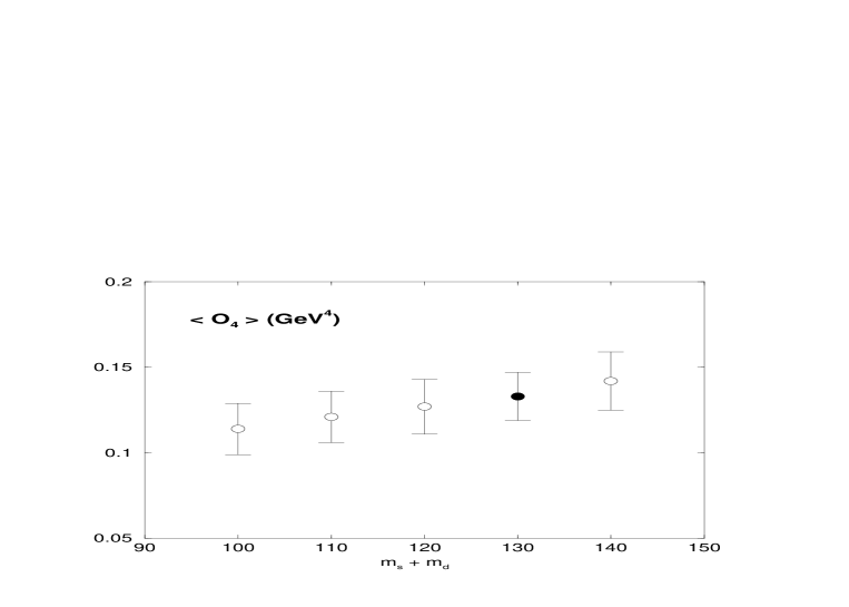
Figure 1: $\langle\bar{K}^{0}|O_{4}|K^{0}\rangle$ in GeV⁴ computed with the new parameterization as a function of the sum of the quark masses $m_{s}+m_{d}$ renormalized in the $\overline{\mbox{MS}}$ scheme at $\mu=\simeq 2$ GeV. The quark masses span a range of values compatible with theoretical estimates.

By forming suitable ratios of the above correlations and looking at their asymptotic behavior at large time separations, one can directly obtain the $B$-parameters defined in eqs. (5). At the leading order in the chiral expansion, or using the definitions of ref. [16], one finds (for $i=2,3,4,5$)

$$R_{i} = \frac{G_{O_{i}}(t_{x},t_{y},\vec{p},\vec{q})}{G_{P}(t_{x},\vec{p})G_{P}(t_{y},\vec{q})}\to\frac{\langle\bar{K}^{0}(\vec{q})|{O}_{i}|K^{0}(\vec{p})\rangle}{|\langle 0|P|K^{0}\rangle|^{2}}=\mbox{const.}\times B_{i}(\mu)\,.$$ (25)

On the other hand, quark masses are extracted using vector or axial-vector Ward identities, e.g.

$$m_{s}(\mu)+m_{d}(\mu) = \frac{\langle 0|\partial_{\nu}A_{\nu}|K^{0}\rangle}{\langle 0|P|K^{0}\rangle}\,,$$ (26)

where the quark masses $m_{s}(\mu)+m_{d}(\mu)$ and the renormalized pseudoscalar density $P$ are given, by definition, in the same renormalization scheme. This happens because matrix elements of the “good” axial currents, and consequently the product $(m_{s}(\mu)+m_{d}(\mu))P$ are regularization, renormalization scheme and scale independent. In practice, for a given renormalization scheme and scale adopted to renormalize $P$, the matrix elements $\langle 0|\partial_{\nu}A_{\nu}|K^{0}\rangle$ and $\langle 0|P|K^{0}\rangle$ are computed numerically and from their ratio one obtains $m_{s}(\mu)+m_{d}(\mu)$.

From a comparison of eqs. (25) and (26), it is evident that, for large values of $\langle 0|P|K^{0}\rangle$, small values of the quark masses and of the $B$-parameters will be simultaneously obtained. The ratio $B_{i}/((m_{s}(\mu)+m_{d}(\mu))^{2}$ , corresponding to the “physical” matrix elements, including the mass factors appearing in eqs. (5), will however be much less dependent on the quark masses since $B_{i}$ and $m_{s}(\mu)+m_{d}(\mu)$ are strongly correlated, i.e. $\langle 0|P|K^{0}\rangle\propto 1/m_{q}$. It would be necessary that calculations of “conventional” $B$-parameters provide at the same time the value of the quark masses obtained in the same calculation. This is equivalent to give, as suggested in eq. (6), the matrix elements in physical units.

In this work we have used the lattice correlation functions computed in [16]. They have been obtained from numerical simulations at $\beta=6.0$ (460 configurations, Run A) and $6.2$ (200 configurations, Run B) with the tree-level Clover action, for several values of the quark masses and for different meson momenta. We have used the “lattice dispersion relation” $\sinh^{2}\left(\frac{E(\vec{p})}{2}\right)=\sinh^{2}\left(\frac{m}{2}\right)+\sum_{i=1,3}\sin^{2}\left(\frac{p_{i}}{2}\right)$. The physical volume is approximatively the same on the two lattices. Statistical errors have been estimated with the jackknife method.

The main numerical results that we have obtained are listed in table 1. They have been computed in the RI(MOM) scheme at $\mu=2$ GeV as follows:

• In the first two columns of the table the results, obtained with the new parameterization, are given. The $\tilde{B}$-parameters are obtained by extrapolating/interpolating the ratios

  $$R^{\prime}_{i}=\frac{M^{2}_{P}}{M^{2}_{V}}\frac{G_{O_{i}}(t_{x},t_{y},\vec{p},\vec{q})}{G_{A}(t_{x},\vec{p})G_{A}(t_{y},\vec{q})}\to\frac{\langle\bar{K}^{0}(\vec{q})|{O}_{i}|K^{0}(\vec{p})\rangle}{M_{V}^{2}f^{2}_{P}}\;.$$ (27)

  to the physical point using the lattice-plane method [32]. $M_{P}$ and $M_{V}$ are the masses of the pseudoscalar and vector mesons computed at the same quark masses as the correlation functions. Then the matrix elements $\langle O_{i}\rangle$ in GeV⁴ are obtained from eq. (8). The standard $B_{i}$’s given in these columns are obtained from eqs. (5) by using the matrix elements in GeV⁴ in the same column and a “conventional” quark mass $(m_{s}+m_{d})^{\overline{MS}}(2\;GeV)=130$ MeV. This is the value of the strange quark mass that we have obtained on the same sets of data [33].

• In the last two columns we show the results obtained with the “conventional” method in ref. [16] on the same set of data. In this case we first obtain the $B$-parameters, defined as in eq. (5), using the procedure described in [16]. The matrix elements in GeV⁴ reported in these columns are derived from the ”conventional” B-parameters in eqs. (5) with the same quark as before of $(m_{s}+m_{d})^{\overline{MS}}(2\;GeV)=(130\pm 15)$ MeV. In this case we have to include the uncertainty coming from the error in the determination of the quark mass. The errors on the $B$-parameters and the quark masses are considered as independent to mimic what is usually done in phenomenological analyses.

The results in table 1 show the convenience of the approach proposed in this paper. Most phenomenological analyses, which use the standard procedure, adopt values of $B$-parameters and quark masses taken from different determinations. For example the $B$-parameter is taken from a calculation at a fixed value of the lattice spacing in the quenched approximation whereas the quark mass is taken from some compilation of lattice results extrapolated to the continuum and including some evaluation of the quenching errors. In other cases, the value of the $B$-parameter is a sort of average biased by results from the large $N$ approach and lattice calculations and the mass is taken from an average from lattice and QCD sum rules. In this way, one misses the correlation between the value of the $B$-parameter and the mass. As a result, the uncertainty on the physical matrix element is much larger. In figure 1 we present the values of the matrix element $\langle\bar{K}^{0}|O_{4}|K^{0}\rangle$ obtained with the new parameterization for different choices of $m_{s}+m_{d}$, in a range of values compatible with theoretical estimates. To be more specific we have computed $\langle\bar{K}^{0}|O_{4}|K^{0}\rangle$ for different values of $m_{s}+m_{d}$, where $m_{s}$ and $m_{d}$ are the masses of the quarks in the meson. This means that different choices of $m_{s}+m_{d}$ also correspond to different values of $M_{K^{0}}$ (and of $f_{K}$).
Although we have data at two different values of the lattice spacing, the statistical errors, and the uncertainties in the extraction of the matrix elements, are too large to enable any extrapolation to the continuum limit $a\to 0$ : within the precision of our results we cannot detect the dependence of $\tilde{B}$-parameters on $a$. For this reason, we estimate the central values by averaging the $B$-parameters obtained with the physical mass $M_{K}^{exp}$ at the two values of $\beta$. Since the results at $\beta=6.0$ have smaller statistical errors but suffer from larger discretization effects, we do not weight the averages with the quoted statistical errors but simply take the sum of the two values divided by two. As far as the errors are concerned we take the largest of the two statistical errors. This is a rather conservative way of estimating the errors. In order to compare the results of Run A and Run B, we have chosen the same physical renormalization scale $\mu$. Using estimates of the lattice spacing ($a^{-1}=2.12(6)$ at $\beta=6.0$ and $a^{-1}=2.7(1)$ at $\beta=6.2$) of ref. [33], we have taken $\mu^{2}a^{2}=0.96$ and $\mu^{2}a^{2}=0.62$, corresponding to $\mu=2.08$ GeV and $\mu=2.12$ GeV, at $\beta=6.0$ and $6.2$ respectively. We quote the results as obtained at $\mu=2$ GeV, since the running of the matrix elements between $\mu\sim 2.1$ and $2.0$ is totally negligible in comparison with the final errors.

5 Physical Results

Our best estimates of the matrix elements of $\Delta S=2$ operators in the RI scheme at $\mu=2$ GeV are given in table 2. Note that these matrix elements are enhanced by a factor $\simeq 2\div 12$ with respect to the SM one ($\langle O_{1}\rangle$). For this reason, $K^{0}-\bar{K}^{0}$ mixing is a promising observable to detect signals of new physics at low energy [18, 27].
From the matrix elements obtained non-perturbatively in the RI scheme, we derive the RGI $\tilde{B}$-parameters using continuum perturbation theory at NLO. These have been computed from eqs. (23) with $\alpha_{s}(2\mbox{GeV})=0.31$, corresponding to $\alpha_{s}(M_{Z})=0.118$, evaluated with the appropriate number of active flavors ( $n_{f}=4$ at 2 GeV). The results are given in table 2. This choice mimics what is usually done in phenomenological analyses which use lattice QCD estimates. It corresponds to the assumption that the results in the RI-scheme are the ”physical” matrix elements, up to some undetermined unquenching errors.

Table 2: Matrix elements in GeV⁴ at $\mu=2$ GeV in the RI scheme and their RGI values with $\alpha_{s}^{n_{f}=4}$.

$\langle O_{i}\rangle$	RI	RGI
$\langle O_{1}\rangle$	0.012(3)	0.017(4)
$\langle O_{2}\rangle$	-0.077(10)	-0.050(7)
$\langle O_{3}\rangle$	0.024(3)	0.001(7)
$\langle O_{4}\rangle$	0.142(12)	0.068(6)
$\langle O_{5}\rangle$	0.034(5)	0.038(5)

Our best estimate of the matrix elements of $\Delta I=3/2$ operators in the RI scheme at $\mu=2$ GeV are

$$\langle\pi^{+}|O_{7}^{3/2}|K^{+}\rangle = -(0.015\pm 0.004)\mbox{GeV}^{4}\;,$$

$$\langle\pi^{+}|O_{8}^{3/2}|K^{+}\rangle = -(0.075\pm 0.008)\mbox{GeV}^{4}\;.$$ (28)

Since the analyses of refs. [24], [34]-[39] are done using Wilson coefficients in NDR and HV, by using the matching coefficients between the RI and these schemes [24]

$$\left(\hat{O}_{i}^{3/2}\right)^{\mbox{\scriptsize NDR},\mbox{\scriptsize HV}}=\left(\delta_{ij}-\frac{\alpha_{s}(\mu)}{4\pi}\Delta r_{ij}^{\mbox{\scriptsize NDR},\mbox{\scriptsize HV}}\right)\left(\hat{O}_{j}^{3/2}\right)^{\mbox{\scriptsize RI}}$$ (29)

where

$$\Delta r_{ij}^{\mbox{\scriptsize NDR}}=\left(\begin{array}[]{cc}\frac{2}{3}+\frac{2}{3}\ln 2&-2-2\ln 2\\ 2-2\ln 2&-\frac{34}{3}+\frac{2}{3}\ln 2\end{array}\right)\;\;\Delta r_{ij}^{\mbox{\scriptsize HV}}=\left(\begin{array}[]{cc}-\frac{8}{3}+\frac{2}{3}\ln 2&-8-2\ln 2\\ -2-2\ln 2&-\frac{62}{3}+\frac{2}{3}\ln 2\end{array}\right).$$

and the results in (5), we have computed the matrix elements $\langle\pi^{+}|O^{3/2}_{i}|K^{+}\rangle$ given in table 3.

Table 3: Matrix elements in GeV⁴ at $\mu=2$ GeV in the NDR and HV schemes and with $\alpha_{s}^{n_{f}=4}(2\mbox{GeV})=0.31$.

$\langle O^{3/2}_{i}\rangle$	NDR	HV
$\langle\pi^{+}|O^{3/2}_{7}|K^{+}\rangle$	-0.021(4)	-0.033(5)
$\langle\pi\pi|O_{7}|K\rangle_{I=2}$	0.11(2)	0.18(3)
$\langle\pi^{+}|O^{3/2}_{8}|K^{+}\rangle$	-0.095(10)	-0.114(12)
$\langle\pi\pi|O_{8}|K\rangle_{I=2}$	0.51(5)	0.62(6)

To obtain $\langle\pi\pi|O_{i}|K\rangle_{I=2}$ we have used the chiral relation of eq. (13). This entails further uncertainty in the numerical evaluation of the physical matrix elements: within our accuracy, we may use in eq. (13) $f_{K}$ instead of $f_{\pi}$. Moreover, to obtain the matrix elements in the $\overline{MS}$ scheme from those obtained non-perturbatively in the RI-scheme, we have chosen the unquenched value $\alpha_{s}(2\mbox{GeV})=0.31$ but, within the quenched approximation, we could have chosen the quenched value of $\alpha_{s}$ as well. We estimate that, due to these effects, the final error is about twice that quoted in table 3.
It is interesting to compare our result for $\langle\pi^{+}|O^{3/2}_{7}|K^{+}\rangle$ in the NDR scheme with the recent estimate from large $N$ expansion [40]. The two determinations differ by more than two $\sigma$ with respect to the error quoted in table 3.

6 Conclusions

In this work we have introduced a new parameterization of four fermion operator matrix elements which does not involve quark masses and thus allows a reduction of systematic uncertainties. As a result the apparent quadratic dependence of $\epsilon^{\prime}/\epsilon$ on the strange quark mass is removed. We have also defined Renormalization Group Invariant matrix elements to simplify the matching between the lattice and continuum renormalization schemes. We have used these definitions to compute matrix elements of $\Delta I=3/2$ and SUSY $\Delta S=2$ four fermion operators on the lattice in the quenched approximation. The simulations have been performed at two different values of the lattice spacing and the renormalization constants of the operators are calculated non perturbatively.

References

- [1] N. Cabibbo, G. Martinelli and R. Petronzio, Nucl. Phys. B244 (1984) 381.
-
[2]
R.C. Brower, M.B. Gavela, R. Gupta and G. Maturana,
Phys. Rev. Lett. 53 (1984) 1318. -
[3]
C. Bernard, Argonne 1984, Proceedings of Gauge
Theory on a Lattice,
p.85-101, UCLA-84-TEP-03. - [4] M. Bochicchio et al., Nucl. Phys. B262 (1985) 331.
- [5] S. Sharpe et al., Nucl. Phys. B286 (1987) 253.
- [6] G. Kilcup, S. Sharpe, R. Gupta and A. Patel, Phys. Rev. Lett. 64 (1990) 25.
-
[7]
N. Ishizuka et al., Nucl. Phys. B (Proc. Suppl.) 34 (1994) 403;
Phys. Rev. Lett. 71 (1993) 24. - [8] S. Aoki et al., Phys. Rev. Lett.80 (1998) 5271
-
[9]
S.R. Sharpe, Nucl. Phys. B (Proc. Suppl.) 53 (1997) 181; R. Gupta,
Invited talk given at 16th Autumn School and Workshop on Fermion Masses,
Mixing and CP Violation (South European Schools on
Elementary Particle Physics) (CPMASS 97), Lisbon, Portugal, 6-15 Oct 1997,
hep-ph/9801412.
L. Lellouch (CERN), Invited talk at 34th Rencontres de Moriond: Electroweak Interactions and Unified Theories, Les Arcs, France, 13-20 Mar 1999, hep-ph/9906497. - [10] C. Bernard et al., Nucl. Phys. B (Proc. Suppl.) 4 (1988) 483.
- [11] E. Franco et al., Nucl. Phys. B317 (1989) 63.
-
[12]
M. B. Gavela et al., Nucl. Phys. B 306 (1988) 677;
Nucl. Phys. B (Proc. Suppl.) 17 (1990) 769. -
[13]
C. Bernard and A. Soni, Nucl. Phys. B (Proc.
Suppl.) 17 (1990) 495;
Nucl. Phys. B (Proc. Suppl.) 42 (1995) 391. - [14] G. Martinelli et al., Nucl. Phys. B445 (1995) 81; A. Donini et al., Phys. Lett. B360 (1996) 83; M. Crisafulli et al., Phys. Lett. B369 (1996) 325; L. Conti et al., Phys. Lett. B421 (1998) 273.
- [15] T. Bhattacharya, R. Gupta and S. Sharpe, Phys. Rev. D55 (1997) 4036.
- [16] C. R. Allton et al., Phys. Lett. B 453 (1999)30.
-
[17]
G. Kilcup,
Nucl. Phys. B (Proc. Suppl.) 20 (1991) 417;
S. Sharpe, Nucl. Phys. B (Proc. Suppl.) 20 (1991) 429;
T. Blum et al., hep-lat/9808025. - [18] M. Ciuchini et al., JHEP 9810:008,1998.
- [19] A. Buras, M. Jamin, M. E. Lautenbacher, Nucl. Phys. B 408 (1993) 209.
- [20] M. Ciuchini, E. Franco, G. Martinelli, L. Reina, Nucl. Phys. B 415 (1994) 403.
-
[21]
W.A. Bardeen, A.J. Buras and J.M. Gérard, Phys. Lett. B 180
(1986) 133; Nucl. Phys. B 293 (1987) 787; Phys. Lett. B 192 (1987) 138.
E.A. Paschos and Y.L. Wu, Mod. Phys. Lett. A6 (1991) 93. -
[22]
R. D. Kenway,
Nucl. Phys. (Proc.Suppl.) 73 (1999) 16 and reference therein.
T. Bhattacharya and R. Gupta, Nucl. Phys. (Proc.Suppl.) 63 (1998)95.
S. R. Sharpe, Talk given at 29th International Conference on High-Energy Physics (ICHEP 98), Vancouver, Canada 1998, HEP Vol. 1 p. 171.
V. Lubicz, Nucl. Phys. (Proc.Suppl.) 74 (1999) 291. -
[23]
G. Martinelli, C. Pittori, C.T. Sachrajda, M. Testa and
A. Vladikas,
Nucl. Phys. B445 (1995) 81. - [24] M. Ciuchini et al., Z. Phys. C68 (1995) 239.
-
[25]
F. Gabbiani, E. Gabrielli, A. Masiero and L. Silvestrini,
Nucl. Phys. B 477 (1996) 321. - [26] J. Bagger, K. Matchev and R. Zhang, Phys. Lett. B 412 (1997) 77.
- [27] L. Giusti, A. Romanino and A. Strumia , Nucl. Phys. B 550 (1999)3.
- [28] M. Ciuchini et al., Nucl. Phys. B 523 (1998) 501.
-
[29]
A. Gonzalez Arroyo, F.J. Yndurain and G. Martinelli,
Phys. Lett. B 117 (1982) 437; Erratum-ibid. B 122 (1983) 486. - [30] S. Capitani et al., Nucl. Phys. B 544 (1999) 669.
-
[31]
A. Donini, V. Gimenez, G. Martinelli, M. Talevi and A. Vladikas,
Eur. Phys. J. C 10 (1999) 121. - [32] C.R. Allton, V. Gimenez, L. Giusti, F. Rapuano, Nucl. Phys. B 489 (1997)427.
- [33] V. Gimenez, L. Giusti, F. Rapuano, M. Talevi, Nucl. Phys. B 540 (1999)472.
- [34] M. Ciuchini, Nucl. Phys. (Proc. Suppl.) 59 (1997) 149.
- [35] A. Buras, M. Jamin and M.E. Lautenbacher, Phys. Lett. B 389 (1996) 749.
- [36] S. Bertolini, J.O. Eeg and M. Fabbrichesi, Nucl. Phys. B 476 (1996) 225.
- [37] S. Bertolini, J.O. Eeg, M. Fabbrichesi and E.I. Lashin, Nucl. Phys. B 514 (1998) 93.
- [38] S. Bosch et al., hep-ph/9904408.
- [39] T. Hambye, G.O. Köhler, E.A. Paschos and P.H. Soldan, hep-ph/9906434.
- [40] M. Knecht, S. Peris and E. de Rafael Phys. Lett. B 457 (1999) 227.