Monte Carlo Renormalization Group analysis of QCD in two dimensional coupling space

Abstract

We report our results of the Monte Carlo Renormalization Group analysis in two dimensional coupling space. The qualitative features of the RG flow are described with a phenomenological RG equation. The dependence on the lattice spacing for various actions provides the conditions to determine the parameters entering the RG equation.

1 Strategy and previous results

The Monte Carlo Renormalization Group (MCRG) approach has been applied to investigate the QCD dynamics under the renormalization transformation and to develop improved lattice actions which enable us to carry out simulations close to the continuum limit even on rather course lattices. In the multi-dimensional coupling space, an action $S$ is transformed from one point to another point under the blocking transformation. There is a special trajectory (renormalised trajectory: RT) which starts from the ultra-violet fixed point and on which actions keep long range contents corresponding to continuum physics. Recently Hasenfratz and Niedermayer reminded us of this fact and called the action on the RT a “perfect action” [1].

This report summarises our previous MCRG study of QCD in two-dimensional coupling space and proposes a model equation to describe the observed flow features. The action takes the form

$$S= \beta_{11}\sum_{plaq}(1-\frac{1}{3}\mbox{ReTr}U_{plaq})$$ (1)

$$+ \beta_{12}\sum_{rect}(1-\frac{1}{3}\mbox{ReTr}U_{rect})$$

where “plaq” and “rect” mean $1\times 1$ and $1\times 2$ loops respectively. We apply the Swendsen’s blocking transformation [2] and determine the couplings of resultant action $S^{\prime}$ by the Schwinger-Dyson equation method [3]. In Fig. 1 the coupling flow under a factor 2 blocking transformation is expressed as arrows [4]. The observed attractive flow to a narrow stream indicates that the RT lies near the present coupling space. This fact was shown more manifestly by performing simulations in the three-dimensional coupling space which contains the 3D twist operator in addition to the plaquette and rectangular loops [5]: Starting from the plane $(\beta_{11},\beta_{12},\beta_{twist}\!=\!0)$, the departure from this plane is small and flow features are almost the same as the ones obtained in two coupling space.

It is hence expected that actions lying on the RT of the 2D coupling space actually reduce the finite lattice spacing effects. To examine this, we defined the DBW2 action (doubly blocked Wilson action in 2D coupling space) through the line defined by the points obtained with successive twice blocking from the Wilson action [6]. In Fig. 1, DBW2 is represented by a dotted line as well as Iwasaki and Symanzik actions [7, 8]. We analysed the rotational symmetry restoration effect and the scaling of $T_{c}$ with the coupling, and found that DBW2 actually improves these quantities.

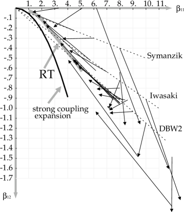
Figure 1: Coupling flow in two-dimensional space.

2 Model equation of flow

We try to describe the observed flow in terms of a model equation which contains a marginal and a irrelevant coupling.

Let us start in the weak coupling region. We adopt the following equation:

$${d\vec{\beta}\over d{\rm ln}a}={\bf A}\vec{\beta}-B(\beta_{n}){\vec{n}\over|\vec{n}|^{2}}.$$ (2)

where $\vec{\beta}={}^{t}(\beta_{11},\beta_{12})$ and $\beta_{n}=(\vec{n}\cdot\vec{\beta})$ . Due to asymptotic scaling, the constant $2\times 2$ matrix ${\bf A}$ has eigenvalues $\lambda=0$ and $\lambda<0$ (irrelevant) with eigenvectors $\vec{w}$ and $\vec{v}$ respectively. $B(x)=12b_{0}+72b_{1}/x$ with $b_{0}=33/(48\pi^{2})$ and $b_{1}=(102/121)b_{0}^{2}$. $\vec{n}$ is a constant vector orthogonal to $\vec{v}$.

In eq.(2), the two-loop asymptotic scaling holds for $\beta_{n}$ as

$$a\Lambda=({\beta_{n}/6+b_{1}/b_{0}\over b_{0}})^{b_{1}/2b_{0}^{2}}\,\exp(-\beta_{n}/12b_{0}).$$ (3)

To obtain the model equation in the strong coupling region, let us consider the strong coupling calculation of Wilson loops in two coupling space.

$$\langle W(N\times M)\rangle = (\beta_{12}/18)^{NM}$$ (4)

$$+(\beta_{12}/18)^{NM-2}(\beta_{12}/18)P_{1}^{NM}+\cdots.$$

where $P_{k}^{NM}$ are tiling weights for filling the area by $(NM-2k)$ [$1\times 2$] and $k$ [$1\times 1$] tiles. Imposing the area law with physical string tension $\sigma$, the $N\times M$ Wilson loop is expressed as

$$\langle W(N\times M)\rangle=\exp(-a^{2}\sigma NM+b(N+M)+c).$$ (5)

For $\beta_{12}=0$, these equations require $\beta_{11}/18=\exp(-a^{2}\sigma)$ in the leading order of $NM$. Then for finite $\beta_{12}$, $\beta_{12}/18=C\exp(-2a^{2}\sigma)$ follows to the same order.

Thus the model equation in the strong coupling region is as follows.

$${d\vec{\beta}\over da^{2}}=-\left(\begin{array}[]{cc}\sigma+\zeta_{1}/a&0\\ 0&2\sigma+\zeta_{2}/a\\ \end{array}\right)\vec{\beta}\ \ ,$$ (8)

where we include the next order contributions with parameters $\zeta_{1}$ and $\zeta_{2}$.

Combining equations (2) and (6), we come to the following RG equation in terms of a dimensionless variable $a_{s}=a\sqrt{\sigma}$:

$${d\vec{\beta}\over da_{s}}= - 2\left(\begin{array}[]{cc}a_{s}+\bar{\zeta_{1}}&0\\ 0&2a_{s}+\bar{\zeta_{2}}\\ \end{array}\right)\vec{\beta}$$ (11)

$$+ {1\over a_{s}}\left[{\bf A}\vec{\beta}-B(\beta_{n}){\vec{n}\over|\vec{n}|^{2}}\right]$$ (12)

where $\bar{\zeta}_{i}=\zeta_{i}/\sqrt{\sigma}$.

The two vectors $\vec{v}$ and $\vec{w}$ are parameterised as $\vec{v}=(\cos\theta^{\prime},\sin\theta^{\prime})$ and $\vec{w}=(\cos\theta,\sin\theta)$ . Then the matrix ${\bf A}$ with a zero and a finite eigenvalue $\lambda$ is given by

$${\bf A}={\lambda\over(\vec{v}\cdot\vec{w_{T}})}\vec{v}\otimes\vec{w_{T}}^{t}$$ (13)

where $\vec{w_{T}}$ is a vector orthogonal to $\vec{w}$. The vector $\vec{n}$ is given by $\vec{n}=(1,\cot(-\theta^{\prime}))$.

We fit the results of [6, 9, 10] to this RG equation. Preliminary results of the fit are shown in Figs. 2 and 3. To show the qualitative features, we use $\theta=-0.156$, $\theta^{\prime}=-0.205$, $\lambda=-0.5$, $\bar{\zeta_{1}}=0.1$ and $\bar{\zeta_{2}}=0.0$. These parameter values are not the result of well-tuned fit. Figure 2 shows $\beta_{11}$ vs $a\sqrt{\sigma}$. Filled symbols are fitted data while open symbols are results of the fit. In Fig. 3, the flow described by the model equation is displayed. These results indicate that the qualitative features of the flow are well described.

Figure 2: $\beta_{11}$ vs $a_{s}=a\sqrt{\sigma}$. Filled symbols: fitted data, Open symbols: results of fit .

Figure 3: Coupling flow described by the model equation. Values of the parameters are found in the text.

3 Conclusions and outlook

In this proceedings, we summarise our previous works on the MCRG analysis in two dimensional coupling space and propose a model equation which, although sufficiently simple to handle, describes well the features of the observed RG flow. A more quantitative analysis will obtain the renormalization trajectory in two-coupling space on which the action is expected to contain quite small finite lattice spacing effects.

The calculations have been done on AP1000 at Fujitsu Parallel Computing Research Facilities, Fujitsu VPP/500 at KEK. This work is supported by the Grant-in-Aide for Scientific Research by Monbusho, Japan (No. 11694085).

References

- [1] P. Hasenfratz and F. Niedermayer, Nucl. Phys. B 414 (1994) 785.
- [2] R.H. Swendsen, Phys. Rev. Lett. 47 (1981) 1775.
- [3] A. González-Arroyo and M. Okawa, Phys. Rev. D 35 (1987) 672; Phys. Rev. B 35 (1987) 2108.
- [4] QCD-TARO (Ph. de Forcrand et al.) “Renormalization group flow of SU(3) gauge theory” HUPD 9817, hep-lat/9806008.
- [5] QCD-TARO (Ph. de Forcrand et al.), Nucl. Phys. B (Proc. Suppl.) 63 (1998) 928.
- [6] QCD-TARO (Ph. de Forcrand et al.), Nucl. Phys. B (Proc. Suppl.) 73 (1999) 924.
- [7] Y. Iwasaki, Univ. of Tsukuba preprint, UTHEP-118, 1983.
- [8] K. Symmanzik, Nucl. Phys. B 226 (1983) 187, 205.
- [9] A. Borici and R. Rosenfelder, Nucl. Phys. B (Proc. Suppl.) 63 (1998) 925.
- [10] CP-PACS Collaboration (M. Okamoto et al.), hep-lat/9905005.