The Weak-Coupling Limit of $3D$ Simplicial Quantum Gravity

Abstract

We investigate the weak-coupling limit, $\kappa\rightarrow\infty$, of $3D$ simplicial gravity using Monte Carlo simulations and a Strong Coupling Expansion. With a suitable modification of the measure we observe a transition from a branched polymer to a crinkled phase. However, the intrinsic geometry of the latter appears similar to that of non-generic branched polymer, probable excluding the existence of a sensible continuum limit in this phase.

1 INTRODUCTION

$D$–dimensional simplicial quantum gravity is a discretization of Euclidean quantum gravity with the integration over space-time metrics replaced by a sum over all possible $D$–dimensional triangulations constructed by gluing together equilateral simplexes. It is defined by the partition function

$$Z(\mu,\kappa)\;=\;\sum_{N_{D}}\;e^{-{\mu}N_{D}}\;Z({\kappa},N_{D})$$ (1)

$$\hskip 37.0pt=\sum_{N_{D},N_{0}}\;e^{-{\mu}N_{D}+{\kappa}N_{0}}\;W_{D}(N_{0},N_{D})\;,$$

$$W_{D}(N_{0},N_{D})\;=\sum_{T\in{\cal T}(N_{0},N_{D})}\frac{1}{C_{T}}\;,$$ (2)

where $N_{D}$ = # $D$–simplexes, $N_{0}$ = # vertices, and $C_{T}$ is the symmetry factor of a labeled triangulation $T$ chosen from a suitable ensemble $\cal T$ (eg combinatorial). $\mu$ and $\kappa$ are the discrete cosmological and Newton’s coupling constants.

In $D=3$ and 4 this model has two phases:

• $\kappa<\kappa_{c}$ : a (intrinsically) crumpled phase

• $\kappa>\kappa_{c}$ : a branched polymer phase

separated (regrettably) by a discontinuous phase transition [1].

As a discontinuous phase transition excludes a sensible continuum limit, there have been several attempts to modify the model Eq. (1) in the hope of finding a non-trivial phase structure. This includes: adding a measure term [2]

$$W_{D}(N_{0},N_{D},{\beta})\;=\sum_{T\in{\cal T}(N_{0},N_{D})}\frac{1}{C_{T}}\;{\prod_{i=0}^{N_{0}}q_{i}^{{\;\beta}}},$$ (3)

where $q_{i}$ is the order of the vertex $i$ (number of simplexes containing $i$), and coupling matter fields to the geometry [3].

Such modifications do indeed lead to a more complicated phase diagram (Fig. 1), and suitable modified the model exhibits a new crinkled phase. But does this new phase structure imply a more interesting non-trivial critical behavior? To investigate this we have studied the weak-coupling limit, $\kappa\rightarrow\infty$, of the model Eq. (1) for $D=3$.

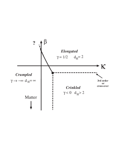
Figure 1: A schematic phase diagram of simplicial gravity in 3 and 4 dimensions.

2 THE EXTREMAL ENSEMBLE

In the weak-coupling limit the partition function Eq. (1), in $D=3$ and 4, is expected to be dominated by an Extremal Ensemble (EE) of triangulations. For this ensemble, defined as triangulations with the maximal ratio $N_{0}/N_{D}$, the partition function simplifies:

$$Z(\mu)\;\;=\;\sum_{N_{D}}\;{\rm e}^{-\mu N_{D}}\;W_{D}(N_{D})$$ (4)

$$W_{D}(N_{D})\;=\sum_{T\in{\cal T}(N_{0}^{\rm max},N_{D})}\;\frac{1}{C_{T}}$$

where

$$N_{0}^{\rm max}\;=\;\left\{\begin{array}[]{cc}\left\lfloor\frac{\textstyle N_{3}+10}{\textstyle 3}\right\rfloor&D=3\;,\\ \vspace{-5pt}\hfil\\ \left\lfloor\frac{\textstyle N_{4}+18}{\textstyle 4}\right\rfloor&D=4\;.\end{array}\right.$$ (5)

Here $\lfloor x\rfloor$ denotes the floor function — the biggest integer not greater than $x$. This in turn defines several distinct series for the EE:

$$3D\;:\;\;S^{0}\;\bigl{(}N_{0},\;3N_{0}\!-\!10\bigr{)},\;\;S^{1}\;\bigl{(}N_{0},\;3N_{0}\!-\!9\bigr{)},$$

$$\hskip 30.0ptS^{2}\;\bigl{(}N_{0},\;3N_{0}\!-\!8\bigr{)}.$$

$$4D\;:\;\;S^{0}\;\bigl{(}N_{0},\;4N_{0}\!-\!18\bigr{)},\;\;\;S^{1}\;\bigl{(}N_{0},\;4N_{0}\!-\!17\bigr{)}.$$

Assuming the asymptotic behavior $W_{D}(N_{D})\sim\exp(-\mu_{c}N_{D})\;N_{D}^{\gamma-3}$, which defines the string susceptibility exponent $\gamma$, we observe (from a SCE) that for the different series $S^{k}$, $\gamma^{k}=k+\frac{1}{2}$. This difference in the exponent $\gamma$ can be understood as the ’higher’ series ($k=1,2,\ldots$) can be constructed by introducing $k$ “defects” (marked points) into triangulations belonging to the minimal series $S^{0}$. Moreover, we observe that the minimal series appears to have very small finite-size effects.

The minimal series $S^{0}$ can be explicitly enumerated as it corresponds to $D$–dimensional combinatorial stacked spheres (CSS), ie to the surface of a $(D+1)$–dimensional simplicial cluster. The number of $(D+1)$–dimensional simplicial clusters build out of $n\;(D+1)$ simplexes, rooted at a marked outer face, is given by (where $n=N_{0}-D-1$) [4]

$$e_{D+1,n}\;=\!\!\!\!\!\!\sum_{\scriptscriptstyle\begin{array}[]{c}n_{1}+\cdots+n_{D+1}\\ =n-1\end{array}}\!\!\!\!\!e_{D+1,n_{1}}\cdots e_{D+1,n_{D+1}}$$

$$\hskip 35.0pt=\;\frac{1}{nD+1}\;\left(\begin{array}[]{c}(D\!+\!1)\;n\\ n\end{array}\right)$$ (6)

$$\Rightarrow\;\;\ W_{D}(N_{D})\;=\;\frac{D+2}{N_{D}}\;e_{D+1,\frac{N_{D}-2}{D}}\;.$$ (7)

Expanding this gives

$$W_{3}(N_{3})=\frac{10}{\sqrt{2\pi}\;N_{3}^{5/2}}\left(\frac{256}{27}\right)^{\frac{N_{3}-2}{3}}\left(1+\frac{83}{48}\frac{1}{N_{3}}\right.\cdots$$

$$W_{4}(N_{4})=\frac{6\sqrt{5}}{\sqrt{2\pi}\;N_{4}^{5/2}}\left(\frac{3125}{256}\right)^{\frac{N_{4}-2}{4}}\left(1+\frac{33}{20}\frac{1}{N_{4}}\right.\cdots$$

with $\gamma=1/2$ as expected for branched polymers.

3 A MODIFIED MEASURE

Figure 2: Evidence of a phase transition in the $3D$ EE, Eq. (4), with a modified measure Eq. (3) (Top) The fluctuations in the measure term: $C_{V}$, and (Bottom) in the maximal vertex order: $\chi_{p_{0}}$.

We have investigated the $3D$ EE including a measure term, using both MC simulations and a SCE [5]. We find a continuous phase transition to a crinkled phase at $\beta\approx-1$ (Fig. 2). This is evident in the fluctuations both in the measure term — the “specific heat” $C_{V}$ — and in the maximal vertex order $p_{0}$. Scaling analysis of the peak value of specific heat gives: $C_{V}^{\rm max}\approx a+bN_{3}^{-0.34(4)}$.

To explore the fractal properties of the geometry in the crinkled phase we have measured the variations in $\gamma$ with $\beta$ using several different methods (Fig. 3). As in $D=4$, we find that $\gamma$ becomes negative at $\beta_{c}$ and decreases with $\beta$. Similarly we find a spectral dimension that increase from $d_{s}=4/3$ for $\beta>\beta_{c}$, to $d_{s}\approx 2$ as $\beta\rightarrow\infty$.

Estimates of the intrinsic fractal dimension $d_{H}$ differ, on the other hand, substantially depending on how it is defined — on the direct graph (from a vertex-vertex distribution) or on the dual graph (simplex-simplex distribution). The former yields $d_{H}\rightarrow\infty$, the latter $d_{H}\approx 2$. In addition, we observe that the crinkled phase appears dominated by a gas of sub-singular vertices.

Combined this evidence suggests that the crinkled phase probably corresponds to some kind of non-generic branched polymers phase which makes it unlikely that any sensible continuum limit exist in this phase. This of course does not exclude the possibility that a second phase order transition point exists somewhere on the phase boudary, for example at the end of the first order transition line (Fig. 1).

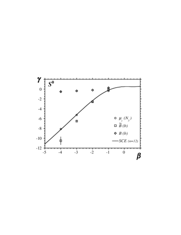
Figure 3: Variations in $\gamma$ with $\beta$ for the EE Eq. (4) with a modified measure Eq. (3).

4 DEGENERATE TRIANGULATIONS

The EE can also be defined with the ensemble of degenerate triangulations introduced in Ref. [6]. In this case degenerate stacked spheres (DSS) are constructed by slicing open a face and inserting a vertex. Different from CSS, Eq. (5), DSS are defined by the maximal ratio:

$$\frac{N_{0}}{N_{D}}\;=\;\frac{1}{2}+\frac{D}{N_{D}}.$$ (8)

This ensemble can also be enumerated explicitly.

Modifying the measure leads to identical phase structure as is observed for CSS. This is shown in Fig. 4 where we plot the variations in $\gamma$ with $\beta$ for the two ensembles. That the two, very different, ensembles agree on the fractal structure is reassuring and reflects the universal properties of the crinkled phase.

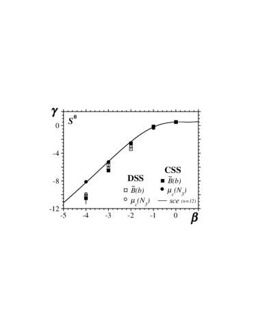
Figure 4: belfig4Variations in $\gamma$ with a modified measure, both for an ensemble of DSS and CSS.

Acknowledgments P. B. was supported by the Alexander von Humboldt Foundation.

References

- [1] G. Thorleifsson, Nucl. Phys. 73 (Proc. Suppl). 73 (1999) 133.
- [2] B. Brugmann and E. Marinari, Phys. Rev. Lett. 70 (1993) 1908.
- [3] S. Bilke, et al, Phys. Lett. B418 (1998) 266; B432 (1998) 279.
- [4] F. Hering, R.C. Read and G.C. Shephard, Discr. Math. 40 (1982) 203.
- [5] G. Thorleifsson, P. Bialas and B. Petersson, Nucl. Phys. B550 (1999) 465.
- [6] G. Thorleifsson, Nucl. Phys. B538 (1999) 278.