$\beta$-function, Renormalons and the Mass Term from Perturbative Wilson Loops UPRF-99-15; BICOCCA-FT-99-29

Abstract

Several Wilson loops on several lattice sizes are computed in Perturbation Theory via a stochastic method. Applications include: Renormalons, the Mass Term in HQET and (possibly) the $\beta$-function.

Outlook

Wilson Loops (WL) were the historic playground (and success …) of Numerical Stochastic Perturbation Theory (NSPT) for Lattice Gauge Theory [1]. Having by now an increased computing power available, we are computing high perturbative orders of various WL on various lattice sizes in Lattice $SU(3)$. Physical motivations range over a variety of issues (not every one within reach, at the moment): Renormalons and Lattice Perturbation Theory (LPT), the Mass Term in Heavy Quark Effective Theory (HQET) and the Lattice $\beta$-function.

1 Renormalons and LPT

In  [2] WL of sizes $1\times 1$ and $2\times 2$ were computed in LPT via NSPT up to $\beta^{-8}$ order. The expected Renormalon contribution was found according to the formula ($Q=a^{-1}$)

$$W_{0}^{\rm ren}={\cal N}\;\int^{Q^{2}}_{r\Lambda^{2}}\;{{k^{2}\,dk^{2}}\over{Q^{4}}}\;\alpha_{\sf s}(k^{2})\,.$$ (1)

which is fixed by dimensional and Renormalization Group considerations. (1) can be cast in a form from which a power expansion can be easily extracted (two loop asymptotic scaling is assumed)

$$z=z_{0}(1-{{\alpha_{\sf s}(Q^{2})}\over{\alpha_{\sf s}(k^{2})}}) z_{0}={{1}\over{3b_{0}}}$$ ,

$$z_{0-}=z_{0}(1-{{\alpha_{\sf s}(Q^{2})}\over{\alpha_{\sf s}(r\Lambda^{2})}}) \gamma=2{{b_{1}}\over{b_{0}^{2}}}$$ ,

$$W_{0}^{\rm ren} = C^{\prime}\int_{0}^{z_{0-}}dz\;e^{-\beta z}\;(z_{0}-z)^{-1-\gamma}$$

$$= \sum_{\ell=1}\beta^{-\ell}\{C^{\prime}\Gamma(\ell+\gamma)z_{0}^{-\ell}+{\cal O}(\Lambda^{4}/Q^{4})\}\,,$$

Actually (1) refers to some continuum scheme. On a finite lattice (which is what NSPT needs) one has to deal with

$$W_{0}^{\rm ren}(s,N)=C\;\int^{Q^{2}}_{Q_{0}^{2}(N)}\;{{k^{2}\,dk^{2}}\over{Q^{4}}}\;\alpha_{\sf s}(sk^{2})\,.$$ (2)

The factor $s$ in the argument of $\alpha_{\sf s}$ is in charge of the lattice-continuum matching and is expected to be of the order $s\sim\left({{\Lambda_{lat}}\over{\Lambda_{cont}}}\right)^{2}$ with respect to some continuum scheme. An explicit IR cut-off is present, dependent on the lattice size ($Q_{0}(N)=2\pi(Na)^{-1}$, where $N$ is the number of points in any direction). (2) results in a new power expansion

$$W_{0}^{\rm ren}(s,N)=\sum_{\ell}\,C_{\ell}^{\rm ren}(C,s,N)\,\beta^{-\ell}$$ (3)

whose coefficients $C_{\ell}^{\rm ren}(C,s,N)$ are given in terms of incomplete $\Gamma$-functions. In [2] (via a slightly different, equivalent formalism) it was shown that this renormalon contribution can account for the growth of the first $8$ coefficients in the pertubative expansion of the plaquette

$$W^{1\times 1}=\sum_{\ell=1}^{8}c^{1\times 1}_{\ell}\,\beta^{-\ell}$$

i.e. convenient values $C^{*}$ and $s^{*}$ were fitted so that $c^{1\times 1}_{\ell}$ were recognized to be asymptotically the same as $C_{\ell}^{\rm ren}(C^{*},s^{*},8)$ (in [2] computations were performed on a rather small $N=8$ lattice); $C_{\ell}^{\rm ren}(C^{**},s^{*},8)$ (with a different choice for $C$) were also shown to fit the expansion of $W^{2\times 2}$.

Control on this (renormalon) perturbative contribution is crucial in the analysis presented in [3]: once its resummation is subtracted from Monte Carlo data for the plaquette, one is left with a ${\cal O}(\Lambda^{2}/Q^{2})$ contribution rather than the expected ${\cal O}(\Lambda^{4}/Q^{4})$. In order to trust this remarkable result, one would like to further test the asymptotic formula (3) by going to even higher orders in the perturbative expansion on various lattice sizes.

By now we know the expansion of the basic plaquette up to order $\beta^{-10}$ on both $N=8$ and $N=24$ lattices. We do not present here the definitive results (which will be published soon elsewhere), but we do show how well the new results are described by $C_{\ell}^{\rm ren}(C^{*},s^{*},N)$ (i.e. by the values for $C$ and $s$ that were fitted in [2, 3]). In the figure the expected $C_{\ell}^{\rm ren}(C^{*},s^{*},24)$ are plotted together with the computed $c^{1\times 1}_{\ell}$ ($\ell=1\ldots 10$) for the $N=24$ lattice. The renormalon contribution is indeed there just like described in [2]. Work is in progress to perform the whole analysis of [3] on the $N=24$ lattice.

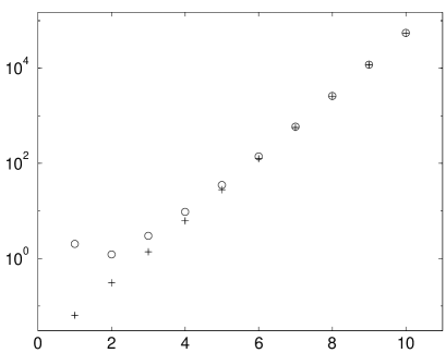
Figure 1: $c^{1\times 1}_{\ell}$ obtained on a $N=24$ lattice (circles) and $C_{\ell}^{\rm ren}(C^{*},s^{*},24)$ (crosses) vs perturbative order ${\ell}$.

2 The Mass Term in HQET

Consider WL of various sizes (in particular square $L\times L$ loops). From their renormalization properties [4] one has to expect

$$W(L)=\exp^{-4M\,L}\;w(L)$$ (4)

The first factor is the exponential of the perimeter times the Mass Term one has to deal with in HQET (an additive, linearly divergent mass renormalization). $w(L)$ contains logarithmic divergences, in particular only those connected to the coupling renormalization is there is no “corner” (which is not the case on the lattice). As stressed in Hashimoto’s review at this conference [5] (after [6]), the mass term is a fundamental building block in a renormalon-safe determination of the b-quark mass from the lattice.

The mass term could of course be determined from the heavy quark propagator. The determination we are going to report on (again after [6]) goes through the computation of various WL and is well suited for NSPT as it is gauge invariant [7]. By computing perturbative expansions of WL of various sizes

$$W(L)=1-W_{1}(L)\,\beta^{-1}-W_{2}(L)\,\beta^{-2}+\ldots$$

and therefore

$$-\log W(L) = W_{1}(L)\,\beta^{-1}+$$

$$\left(W_{2}(L)+{{1}\over{2}}W_{1}(L)^{2}\right)\beta^{-2}+\ldots$$

one can extract from each order the leading (linear) behaviour in $L$, that is mass term

$$4\,M\,L=4\left(M_{1}\,\beta^{-1}+M_{2}\,\beta^{-2}+\ldots\right)L\,.$$ (5)

At the moment we have got results for square loops on a $(N=24)^{4}$ lattice. Results on bigger lattices ($N=28,32$) and rectangular loops are expected to come soon. They will be crucial to control finite size effects and subleading (logarithmic) contributions. As $M_{1}$ and $M_{2}$ are already known, they have to be recovered. Consider for example $M_{1}$, which has to be recovered by fitting $W_{1}(L)$ to

$$W_{1}(L)=4\,M_{1}\,L+k_{1}\log L+k_{0}$$

The analytical result is $M_{1}=1.01$ and we get $M_{1}=1.00\pm 0.02$. From [6] one learns the second coefficient $M_{2}=2.54$, while from our fits we get $M_{2}=2.43\pm 0.15$. The errors we quote depend on both finite size effects and fitting subleading contributions. Note that since $W_{3}(L)$ contains a $(\log L)^{2}$ contribution, the latter point is even more crucial in the determination of $M_{3}$. At the moment we can pin down a preliminary number $M_{3}=8\pm 1$ which will turn in a definite number as soon as we get definite results not only for square loops, but also for ratios of rectangular loops.

3 The Lattice $\beta$-function

We now turn to describe what could possibly be another application of our perturbative computations. Ratios of WL combined in such a way that the corner and mass contributions cancel out were introduced several years ago by Creutz [8] in order to study (among other things) the non-perturbative Lattice $\beta$-function.

Consider rectangular WL of sizes $(L,L)$, $(2L,L)$, $(2L,2L)$ on a $(4L)^{4}$ lattice and form the ratio

$${\cal R}(L) = {{W(L,L)\,W(2L,2L)}\over{W(L,2L)^{2}}}$$

$$= 1+c_{1}(L)\,\alpha_{0}+c_{2}(L)\,\alpha_{0}^{2}+\ldots$$

where $\alpha_{0}$ is the bare lattice coupling. The only scale is $L$ and the only renormalization needed is that of the coupling, so that (for example)

$$\alpha_{{\cal R}}(L)={{1}\over{c_{1}(L)}}\log({\cal R}(L))$$ (6)

is supposed to be an acceptable coupling running with L. Since the pertubative matching between coupling in different schemes

$$\alpha_{1}(s\mu)=\alpha_{2}(\mu)+d_{1}(s)\,\alpha_{2}(\mu)^{2}+\ldots$$

contains all the informations about the perturbative $\beta$-functions in both schemes, one could in principle study the perturbative Lattice $\beta$-function by computing the perturbative expansion of $\alpha_{CR}(L)$ in $\alpha_{0}$ at different values of $N$, where $L=Na$ (i.e. by computing different WL on different lattice sizes).

Within this application the big issue is accuracy. Due to large cancellations of the mass contribution, a fraction of per mille accuracy on the $c_{i}(L)$ (which is within reach) straight away degenerates when one computes for example $d_{1}(s)$ (still we were able to recover $b_{0}$, the first universal coefficient of the $\beta$-function). In view of this, it is quite unlikely that one can attain the terrific accuracy which should be needed to get the first unknown information. One should most probably look for a smarter definition of the coupling.

Conclusions

Preliminary results were reported, coming from the computations of perturbative expansions of various WL. The basic plaquette is now known up to $\beta^{-10}$ order and the results on Renormalons [2] are indeed to be trusted. Work is in progress to gain further confidence in the results of [3] as well. A preliminary results on third order in the computation of the mass term has been reported and a definite result will be published soon. In principle also the perturbative lattice $\beta$-function could be studied via WL in NSPT, even if the accuracy needed to get the first unknown result is quite unlikely to be attained.

References

- [1] F. Di Renzo, G. Marchesini, P. Marenzoni and E. Onofri, Nucl. Phys. B426 (1994) 675.
- [2] F. Di Renzo, G. Marchesini and E. Onofri, Nucl. Phys. B457 (1995) 202.
- [3] G. Burgio, F. Di Renzo, G. Marchesini and E. Onofri, Phys. Lett. 422B (1998) 219.
- [4] V.S. Dotsenko and S.N. Vergeles, Nucl. Phys. B169 (1980) 527.
- [5] S. Hashimoto, these proceedings.
- [6] G. Martinelli and C.T.S. Sachrajda, hep-lat/9812001.
- [7] For an independent computation see P.B. Mackenzie et al, these proceedings.
- [8] M. Creutz, Phys. Rev. D 23 (1981) 1815.