Electroweak Phase Transitions

Abstract

Recent developments on the four dimensional (4d) lattice studies of the finite temperature electroweak phase transition (EWPT) are summarized. The phase diagram is given in the continuum limit. The finite temperature SU(2)-Higgs phase transition is of first order for Higgs-boson masses $m_{H}<66.5\pm 1.4$ GeV. Above this endpoint only a rapid cross-over can be seen. The full 4d result agrees completely with that of the dimensional reduction approximation. The Higgs-boson endpoint mass in the Standard Model (SM) would be $72.1\pm 1.4$ GeV. Taking into account the LEP Higgs-boson mass lower bound excludes any EWPT in the SM. A one-loop calculation of the static potential in the SU(2)-Higgs model enables a precise comparison between lattice simulations and perturbative results. The most popular extension of the SM, the Minimal Supersymmetric SM (MSSM) is also studied on 4d lattices.

1 INTRODUCTION

The visible Universe is made of matter. This fact is based on observations of the cosmic diffuse $\gamma$-ray background, which could be larger than the present limits, if boundaries between “worlds” and “antiworlds” had existed [1]. The observed baryon asymmetry of the universe was eventually determined at the EWPT [2]. On the one hand this phase transition was the last instance during which baryon asymmetry could have been generated around $T\approx 100$ GeV, on the other hand at these temperatures any B+L asymmetry could have been washed out. The possibility of baryogenesis at the EWPT is a particularly attractive one, since the underlying physics can be –and already largely has been– tested at collider experiments. Thus, the detailed understanding of this phase transition is very important.

A succesfull baryogenesis scenario consists three ingredients, the Sakharov’s conditions.
1. Baryon number violating processes
2. C and CP violation
3. Departure from equilibrium.
All of the three conditions has non-perturbative features and are studied on the lattice (e.g. at this conference baryon number violating sphalerons have been discussed by [3], spontaneous CP violation by [4], whereas this contribution mostly studies the out of equilibrium condition).

It is rather easy to see the necessity of the first two conditions. Without baryon number violation no net baryon asymmetry can be generated. C and CP violation are needed to give a direction to the processes. The standard picture concerning the third condition is the turn-off of the baryon number violating rate after the phase transition, which means a smaller sphaleron rate than the Hubble rate. Inspecting the formula for the sphaleron rate one needs a strong enough phase transition, thus $v/T_{c}\mathop{\raise 1.29167pt\hbox{$>$\kern-7.5pt\raise-4.73611pt\hbox{$\sim$}}}1$. This ratio is of particular interest and both perturbative and lattice studies have the main goal to determine it.

The first-order nature of the EWPT for light Higgs bosons can be shown within perturbation theory. However, perturbation theory breaks down for Higgs boson masses ($m_{H}$) larger than about 60 GeV due to bad infrared behavior of the gauge-Higgs part of the electroweak theory [5]. Solutions of gap-equations even suggest an end-point scenario for the first order EWPT [6]. Numerical simulations are needed to analyze the nature of the transition for realistic Higgs bosons.

One very succesfull possibility is to construct an effective three dimensional (3d) theory by using dimensional reduction, which is a perturbative step. The non-perturbative study is carried out in this effective 3d model [7]. The end-point of the phase transition is determined and its universality class is studied [8].

Another approach is to use 4d simulations. The complete lattice analysis of the SM is not feasible due to the presence of chiral fermions, however, the infrared problems are connected only with the bosonic sector. These are the reasons why the problem is usually studied by simulating the SU(2)-Higgs model on 4d lattices, and perturbative steps are used to include the U(1) gauge group and the fermions. Finite temperature simulations are carried out on lattices with volumes $L_{t}\cdot L_{s}^{3}$, where $L_{t}\ll L_{s}$ are the temporal and spatial extensions of the lattice, respectively. Systematic studies were carried out for $m_{H}\approx$ 20 GeV, 35 GeV, 50 GeV and 75 GeV [9]. The lattice spacing is basically fixed by the number of the lattice points in the temporal direction ($T_{c}=1/(L_{t}a)$, where $T_{c}$ is the critical temperature in physical units); therefore huge lattices are needed to study the soft modes. This problem is particularly severe for Higgs boson masses around the W mass, for which the phase transition is weak and typical correlation lengths are much larger than the lattice spacing. In this case asymmetric lattice spacings are used [10].

2 END-POINT IN FOUR DIMENSIONS

The 4-d SU(2)-Higgs model is studied on both symmetric and asymmetric [10] lattices, i.e. lattices with equal or different spacings in temporal ($a_{t}$) and spatial ($a_{s}$) directions. The asymmetry of the lattice spacings is given by the asymmetry factor $\xi=a_{s}/a_{t}$. The different lattice spacings can be ensured by different coupling strengths in the action for time-like and space-like directions. The action reads in standard notation [9]

$$S[U,\varphi]=$$

$$\beta_{s}\sum_{sp}\left(1-{1\over 2}{\rm Tr\,}U_{pl}\right)+\beta_{t}\sum_{tp}\left(1-{1\over 2}{\rm Tr\,}U_{pl}\right)$$

$$+\sum_{x}\left\{{1\over 2}{\rm Tr\,}(\varphi_{x}^{+}\varphi_{x})+\lambda\left[{1\over 2}{\rm Tr\,}(\varphi_{x}^{+}\varphi_{x})-1\right]^{2}\right.$$

$$\left.-\kappa_{s}\sum_{\mu=1}^{3}{\rm Tr\,}(\varphi^{+}_{x+\hat{\mu}}U_{x,\mu}\,\varphi_{x})\right.$$

$$\left.-\kappa_{t}{\rm Tr\,}(\varphi^{+}_{x+\hat{4}}U_{x,4}\,\varphi_{x})\right\},$$ (1)

We introduce $\kappa^{2}=\kappa_{s}\kappa_{t}$ and $\beta^{2}=\beta_{s}\beta_{t}$. The anisotropies $\gamma_{\beta}^{2}=\beta_{t}/\beta_{s}$ and $\gamma_{\kappa}^{2}=\kappa_{t}/\kappa_{s}$ are functions of $\xi$. We use $\xi=4.052$, which corresponds to $\gamma_{\kappa}=4$ and $\gamma_{\beta}=3.919$.

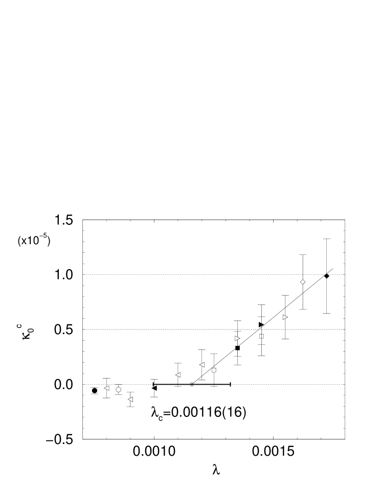
Figure 1: Imaginary part of first Lee-Yang zero as a function of $\lambda$ from simulations on symmetric lattices with $L_{t}=2$. Filled symbols are without $\lambda$-reweighting, while open symbols with $\lambda$-reweighting from filled symbol with same shape.

The determination of the end-point of the finite temperature EWPT is done by the use of the Lee-Yang zeros of the partition function ${\cal Z}$. Near the first order phase transition point the partition function reads ${\cal Z}={\cal Z}_{s}+{\cal Z}_{b}\propto\exp(-Vf_{s})+\exp(-Vf_{b})\ ,$ where the indices s(b) refer to the symmetric (broken) phase and $f$ stands for the free-energy densities. We also have $f_{b}=f_{s}+\alpha(\kappa-\kappa_{c})\ ,$ , since the free-energy density is continuous. It follows that ${\cal Z}\propto\exp[-V(f_{s}+f_{b})/2]\cosh[-V\alpha(\kappa-\kappa_{c})]\ ,$ which shows that for complex $\kappa$ ${\cal Z}$ vanishes at ${\rm Im}(\kappa)=2\pi\cdot(n-1/2)/(V\alpha)$ for integer $n$. In case a first order phase transition is present, these Lee-Yang zeros move to the real axis as the volume goes to infinity. In case a phase transition is absent the Lee-Yang zeros stay away from the real $\kappa$ axis. Denoting $\kappa_{0}$ the lowest zero of ${\cal Z}$, i.e. the position of the zero closest to the real axis, one expects in the vicinity of the end-point the scaling law ${\rm Im}(\kappa_{0})=C(L_{t},\lambda)V^{-\nu}+\kappa_{0}^{c}(L_{t},\lambda)$. In order to pin down the end-point we are looking for a $\lambda$ value for which $\kappa_{0}^{c}$ vanishes. In practice we analytically continue ${\cal Z}$ to complex values of $\kappa$ by reweighting. Small changes in $\lambda$ were taken into account by reweighting. The dependence of $\kappa_{0}^{c}$ on $\lambda$ [11] is shown in fig. 1. To determine the critical value of $\lambda$ i.e. the largest value, where $\kappa_{0}^{c}=0$, we have performed fits linear in $\lambda$ to the non-negative $\kappa_{0}^{c}$ values.

Figure 2: Dependence of $R_{HW,c}$, on $1/L_{t}^{2}$ and extrapolation to the continuum limit.

In the isotropic case [11], we have used $L_{t}=2$. The Lee-Yang analysis gave $\lambda_{c}=0.00116(16)$ for the end-point. Performing $T=0$ simulations with the same parameters this can be converted to $m_{H,c}=73.3\pm 6.4$GeV. In the anisotropic lattice simulation case [12] we also performed a continuum extrapolation for $L_{t}=2,3,4,5$ (fig. 2), moving along the lines of constant physics (LCP), and obtained $66.5\pm 1.4$ GeV, which is our final result for the end-point in the SU(2)-Higgs model.

Based on previous 4d simulation results one can determine the phase diagram of the finite temperature EWPT and compare it with the 3d analysis (fig. 3.) as it has been done in ref. [13]. The phase transition lines $T_{c}(m_{H})$, are in perfect agreement for $m_{H}\mathop{\raise 1.29167pt\hbox{$>$\kern-7.5pt\raise-4.73611pt\hbox{$\sim$}}}25$ GeV. For strong first order phase transition close to the Coleman-Weinberg limit the 3d approach seems to be less accurate. The error bars on the endpoints are on the few percent level, thus uncertainty of the dimensional reduction around the end-point is also in this range. This indicates that the analogous perturbative inclusion of the fermions results also in few percent error on $m_{H}$.

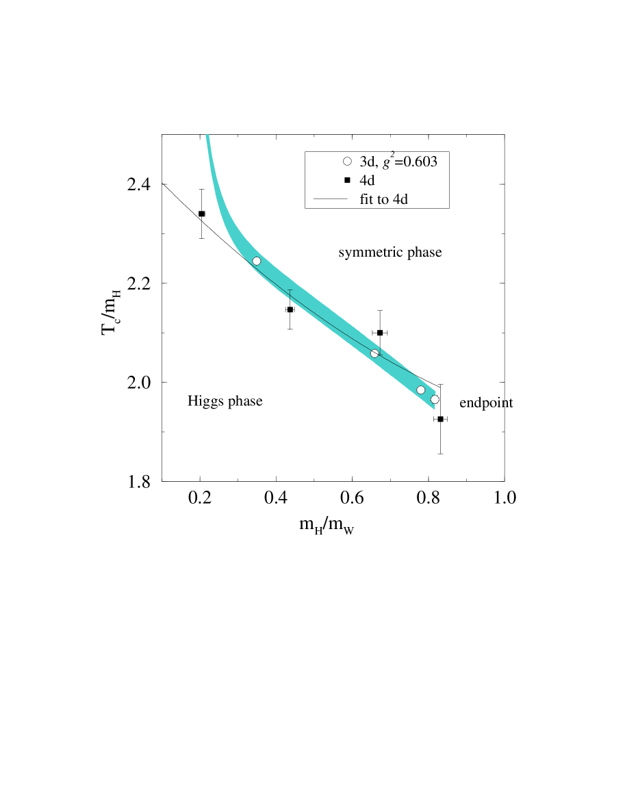
Figure 3: A comparison of the phase diagrams obtained from direct 4d simulations (squares) and from dimensionally reduced 3d simulations (shaded region).

One can determine what is the endpoint value in the full SM. As it was shown previously the perturbative integration of the heavy modes is correct within our error bars. Therefore we use perturbation theory to transform the SU(2)-Higgs model endpoint value to the full SM. We obtain $72.1\pm 1.4$ GeV, where the dominant error comes from the measured error of $R_{HW,cont.}$. The error on $g_{R}^{2}$ is eliminated by calculating the relationship between the coupling definitions used in perturbation theory (${\overline{\rm{MS}}}$) and lattice simulations (from static potential) [13, 14]. The calculation of this relationship and a comparison of the perturbative and lattice results on the EWPT will be shortly discussed in the next section.

The full SM result needs some explanation. Based on vacuum stability the measured top mass ($m_{top}\approx 175$ GeV) results in a lower bound for the Higgs boson mass (approx. 130 GeV). This value is higher than the previously mentioned $72.1\pm 1.4$ GeV. For the pure SU(2)-Higgs model the endpoint Higgs mass is $66.5\pm 1.4$ GeV. The inclusion of the fermions, especially the top increases the endpoint slightly. For a hypothetical top quark mass less than approximately 150 GeV the lower bound is less than $\approx 70$ GeV, thus it is below the endpoint and it gives a reliable theory. Increasing the top quark mass the lower bound gets larger than the endpoint. This means that independently of the direct experimental bounds on the Higgs boson mass no EWPT exists in the SM.

3 RELATIONSHIP BETWEEN GAUGE COUPLINGS

Despite the fact that the perturbative and lattice approaches are systematic and well-defined, it is not easy to compare their predictions. The reason is that in lattice simulations the gauge coupling constant is determined from the static potential, whereas in perturbation theory the ${\overline{\rm{MS}}}$ scheme is used. One can calculate the static potential on the one-loop level in the SU(2)-Higgs model [13, 14]. As expected the numerical difference between the two conventions is not that large, it is within a few percent, for details see [13, 14]. With this connection we could perform a precise comparison between the predictions of perturbative and lattice approaches (fig. 4).

In [14] the existing lattice data was reanalyzed and a continuum limit extrapolation was performed whenever it was possible. The only quantity which is measured so precisely that the definition of the gauge coupling constant is essential is the ratio of the critical temperature to the Higgs boson mass. As it has been observed already for $M_{H}\approx 35$ GeV the perturbative value of $T_{c}$ is larger than in lattice simulations. This sort of discrepancy disappears for larger Higgs boson masses. A plausible reason for this fact is the convergence of the high temperature expansion used in the perturbative approach.

The most dramatic differences appear clearly as we get closer to the end point. The perturbative approach gives non-vanishing jump of the order parameter, non-vanishing latent heat and interface tension, while the lattice results suggest rapid decrease of these quantities and no phase transition beyond the end-point.

Figure 4: Pulls plotted against the Higgs mass for $T_{c}$, $v/T$, latent heat and interface tension.

4 PHASE TRANSITION IN THE MSSM

As it was demonstrated in the previous sections the SM is not suitable for baryogenesis, not even for a first order EWPT. Several extended models were studied in order to obtain a stronger first order phase transition and a reliable baryon asymmetry. The most popular model is the MSSM, which perturbatively shows a much stronger phase transition than the SM [15] (even an intermediate colour breaking phase transition is possible in these scenarios) . Lattice studies in a 3d reduced model (with one Higgs doublet) basically confirmed the perturbative results [16].

We performed a 4d lattice study with the bosonic sector of the MSSM [17]. The lattice action is too long to be presented here, thus only the fields involved are listed. Both of the Higgs doublets, the stop, sbottom scalars and SU(2), SU(3) gauge fields were included. It is of particular importance to keep both of the Higgs doublets, since according to the standard scenario the generated baryon asymmetry is directly proportional to the change of the ratio of their expectation values $n_{B}\propto\langle v^{2}\rangle\Delta\beta(T_{c})$. Here the length squared of the Higgs field ($v^{2}=v_{1}^{2}+v_{2}^{2}$) is integrated over the bubble wall. The ratio of the expectation values of the two Higgs fields is $\tan\beta=v_{1}/v_{2}$, and the difference between the $\beta$ values are taken in the “symmetric” and in the “broken” phases.

We had simulations at $L_{t}=2,3,4,5$ and moved along the line of constant physics. Our simulation point corresponds to $\tan\beta(T=0)\approx 6$, and the mass of the lightest Higgs bosons is approx. 35 GeV (in the bosonic theory).

Two values of $\alpha_{s}$ were taken (the physical and a smaller one). The physical $\alpha_{s}$ resulted in $v/T_{c}\approx 1.5$, whereas the smaller value of $\alpha_{s}$ gave a stronger phase transition $v/T_{c}\approx 2$. Perturbation theory predicts just the opposite behaviour (stop-gluon setting sun graphs are proportional to the strong coupling and they are responsible for the strengthening of the phase transition). The reason can be the difference between the renormalization effects in the stop sector.

We measured the $\beta$ parameter in both phases at the phase transition. One obtains $\tan^{2}\beta(sym)=38.13(15)$, $\tan^{2}\beta(brok)=36.04(15)$, which gives $\Delta\beta=0.0045(7)$. This result is far below the perturbative prediction $\Delta\beta(pert.)=0.017$.

5 CONCLUSIONS

The endpoint of hot EWPT with the technique of Lee-Yang zeros from simulations in 4d SU(2)-Higgs model was determined. The phase transition is first order for Higgs masses less than $66.5\pm 1.4$ GeV, while for larger Higgs masses only a rapid cross-over is expected. The phase diagram of the model was given.

It was shown non-perturbatively that for the bosonic sector of the SM the dimensional reduction procedure works within a few percent. This indicates that the analogous perturbative inclusion of the fermionic sector results also in few percent error. In the full SM we get $72.1\pm 1.4$ GeV for the end-point, which is below the lower experimental bound. This fact is a clear sign for physics beyond the SM.

Based on a one-loop calculation on the static potential of the SU(2)-Higgs model a direct comparison between the perturbative and lattice results was performed.

The MSSM is more promising for a succesfull baryogenesis. Some 4d results were shown, indicating a strong first order phase transition.

Acknowledgments: This work was partially supported by Hung. Grants No. OTKA-T22929-29803-M28413-FKFP-0128/1997.

References

- [1] A.G. Cohen, A. De Rujula, S.L. Glashow, Astrophys. J. 495 (1998) 539.
- [2] V.A. Kuzmin, V.A. Rubakov and M.E. Shaposhnikov, Phys. Lett. B155 (1985) 36.
- [3] D. Bödeker, G.D. Moore, K. Rummukainen, hep-lat/9909054 (these proceedings).
- [4] M. Laine and K. Rummukainen, hep-lat/9908045 (these proceedings).
- [5] P. Arnold and O. Espinosa, Phys. Rev. D47 (1993) 3546, Erratum ibid. D50 (1994) 6662; Z. Fodor and A. Hebecker, Nucl. Phys. B432 (1994) 127; W. Buchmüller, Z. Fodor, and A. Hebecker, Nucl. Phys. B447 (1995) 317.
- [6] W. Buchmüller et al., Ann. Phys. (NY) 234 (1994) 260; W. Buchmüller, O. Philipsen, Nucl. Phys. B443 (1995) 47.
- [7] K. Farakos et al., Nucl. Phys. B425 (1994) 67; A. Jakovác, K. Kajantie and A. Patkós, Phys. Rev. D49 (1994) 6810; K. Kajantie et al., Nucl. Phys. B458 (1996) 90; ibid. B466 (1996) 189; Phys. Rev. Lett. 77 (1996) 2887.
- [8] F. Karsch et al., Nucl. Phys. Proc. Suppl. 53 (1997) 623; M. Gürtler et al., Phys. Rev. D56 (1997) 3888 (1997); K. Rummukainen et al., Nucl. Phys. B532 (1998) 283.
- [9] Z. Fodor et al., Phys. Lett. B334 (1994) 405; Nucl. Phys. B439 (1995) 147; F. Csikor et al., Nucl. Phys. B474 (1996) 421; Phys. Lett. B357 (1995) 156.
- [10] F. Csikor, Z. Fodor, Phys. Lett. B380 (1996) 113; F. Csikor, Z. Fodor and J. Heitger, Phys. Rev. D58 (1998) 094504.
- [11] Y. Aoki et al., Phys. Rev. D60 (1999) 013001.
- [12] F. Csikor, Z. Fodor and J. Heitger, Phys. Rev. Lett. 82 (1999) 21.
- [13] M. Laine, JHEP 9906 (1999) 020, hep-ph/9903513.
- [14] F. Csikor et al., hep-ph/9906260.
- [15] A. Brignole et al., Phys. Lett. B324 (1994) 181; M. Carena, M. Quiros, C.E.M. Wagner, Phys. Lett. B380 (1996) 81; B. de Carlos, J.R. Espinosa, Nucl. Phys. B503 (1997) 24; D. Bödeker et al., Nucl. Phys. B497 (1997) 387; M. Losada, Nucl. Phys. B537 (1999) 3.
- [16] M. Laine, K. Rummukainen, Phys. Rev. Lett. 80 (1998) 5259; Nucl. Phys. B535 (1998) 423.
- [17] F. Csikor, Z. Fodor, P. Hegedűs, V. Horváth, S.D. Katz, A. Piróth, in preparation.