$\Lambda$-parameter of lattice QCD with the overlap-Dirac operator

Abstract

We compute the ratio $\Lambda_{L}/\Lambda_{\overline{MS}}$ between the scale parameter $\Lambda_{L}$, associated with a lattice formulation of QCD using the overlap-Dirac operator, and $\Lambda_{\overline{MS}}$ of the $\overline{\rm MS}$ renormalization scheme. To this end, the necessary one-loop relation between the lattice coupling $g_{0}$ and the coupling renormalized in the $\overline{{\rm MS}}$ scheme is calculated, using the lattice background field technique.

Keywords: Lattice QCD, overlap-Dirac operator, $\Lambda$-parameter, Asymptotic scaling, Lattice perturbation theory.

PACS numbers: 11.15.–q, 11.15.Ha, 12.38.G.

I Introduction

The overlap-Dirac operator [1] that has been derived from the overlap formulation of chiral fermions on the lattice [2] provides a lattice regularization of massless QCD, i.e. of chiral fermions coupled vectorially to a gauge field, without the need of fine tuning. It preserves chiral symmetry without fermion doubling, circumventing the Nielsen-Ninomiya theorem [3]. The overlap-Dirac operator $D_{o}$ of a massless fermion can be written as ($a$ is the lattice spacing)

$$D_{o}={1\over a}\left[1+\gamma_{5}O\right],$$ (1)

where $O$ depends on the link variables, and is Hermitian with eigenvalues $\pm 1$. The simplest such example is given by the Neuberger-Dirac operator [1]

$$D_{\rm N} = {1\over a}\,c\left[1+X(X^{\dagger}X)^{-1/2}\right],$$ (2)

$$X = D_{\rm W}-{1\over a}\rho,$$ (3)

where $D_{\rm W}$ is the Wilson-Dirac operator (with the Wilson parameter $r$ set to its standard value, $r=1$)

$$D_{\rm W}={1\over 2}\left[\gamma_{\mu}\left(\nabla_{\mu}^{*}+\nabla_{\mu}\right)-a\nabla_{\mu}^{*}\nabla_{\mu}\right],$$ (4)

$$\nabla_{\mu}\psi(x)={1\over a}\left[U(x,\mu)\psi(x+a\hat{\mu})-\psi(x)\right],$$ (5)

and $\rho$ is a real parameter subject to the constraint $0<\rho<2$. The normalization constant $c=\rho$ can be absorbed in the definition of the fermion fields. Unlike the Wilson-Dirac operator $D_{\rm W}$, $D_{N}$ is not analytic in the link variables when the operator $X$ in Eq. (3) has a zero eigenvalue. As discussed in Ref. [4], this is the price to pay for putting strictly massless fermions on the lattice. However, such a lack of analiticity is expected to be harmless in the continuum limit [4, 23].

$D_{\rm N}$ satisfies the Ginsparg-Wilson relation [6]

$$\gamma_{5}D+D\gamma_{5}=aD\gamma_{5}D,$$ (6)

which protects the quark masses from additive renormalization [1, 7]. The Ginsparg-Wilson relation allows us to write, at finite lattice spacing, relations that are essentially equivalent to those holding in the low-energy phenomenology associated with chiral symmetry (see e.g. Refs. [8, 9]). It indeed implies the existence of an exact chiral symmetry of the lattice action under the transformation [10]

$$\delta\psi(x)=\gamma_{5}(1-\frac{1}{2}aD)\psi(x),\qquad\qquad\delta\bar{\psi}(x)=\bar{\psi}(x)(1-\frac{1}{2}aD)\gamma_{5},$$ (7)

thus leading to chiral Ward identities that ensure the non-renormalization of vector and flavor non-singlet axial vector currents, and the absence of mixing among operators in different chiral representations. The axial anomaly then arises from the non-invariance of the fermion integral measure under flavour-singlet chiral transformations [10, 11, 12, 13, 14, 15]. It is also worth mentioning that lattice gauge theories with Ginsparg-Wilson fermions have been proved to be renormalizable to all orders of perturbation theory [16].

The important point is that lattice Dirac operators satisfying Eq. (6) are not affected by the Nielsen-Ninomiya theorem [3], thus they need not suffer from fermion doubling. A lattice formulation of QCD satisfying the Ginsparg-Wilson relation would overcome the complications of the standard approach (e.g. Wilson fermions), where chiral symmetry is violated at the scale of the lattice spacing. As a consequence of chiral symmetry, leading scaling corrections are $O(a^{2})$, as opposed to $O(a)$ of the chiral symmetry violating case.

Indeed, $D_{\rm N}$ avoids fermion doubling. However, its locality properties in the presence of a gauge field are not obvious. $D_{\rm N}$ is not strictly local, and locality should be recovered only in a more general sense, i.e. allowing an exponential decay of the kernel of $D_{\rm N}$ with a rate which scales with the lattice spacing and not with the physical quantities. In Ref. [23] the locality of $D_{\rm N}$ has been proved for sufficiently smooth gauge fields. Moreover numerical evidence has been presented for typical gauge fields in present-day simulations. Thus, the Neuberger-Dirac operator seems to have all the right properties that a lattice Dirac operator should have in order to describe massless quarks. A major open question seems to be its practical implementation, since $D_{\rm N}$ appears much more complicated than the usual Wilson-like Dirac operators. In this respect some progress has been achieved (see, e.g., Refs. [17, 23, 18, 19, 20, 4, 21, 22, 23, 24, 25]), and simulations may become feasible in the near future.

In this paper we calculate the ratio between the $\Lambda$-parameter associated with a lattice formulation of QCD using the overlap-Dirac operator ($\Lambda_{L}$) and that of the $\overline{\rm MS}$ renormalization scheme ($\Lambda_{\overline{\rm MS}}$). In order to have a complete discretization of QCD, we will consider the Wilson formulation for the pure gauge part of the theory. Actually, the part of the calculation involving fermions is independent of the regularization chosen for the gluonic part. We recall that the ratio of any renormalization group invariant quantity to the appropriate power of $\Lambda_{L}$ approaches a constant in the continuum limit $g_{0}\rightarrow 0$. Indeed $\Lambda_{L}$ is a particular solution of the renormalization group equation

$$\left(-a{\partial\over\partial a}+\beta_{L}(g_{0}){\partial\over\partial g_{0}}\right)\Lambda_{L}=O(a),$$ (8)

i.e.

$$a\Lambda_{L}=\exp\left[-\int^{g_{0}}{dg\over\beta_{L}(g)}\right]=\exp\left(-{1\over 2b_{0}g_{0}^{2}}\right)(b_{0}g_{0}^{2})^{-{b_{1}/2b_{0}}}\left[1+O\left(g_{0}^{2}\right)\right],$$ (9)

where $\beta_{L}(g_{0})$ is the lattice $\beta$-function, and $b_{0},b_{1}$ the first two coefficients of its perturbative expansion:

$$b_{0}={1\over(4\pi)^{2}}\left({11\over 3}N-{2\over 3}N_{f}\right),$$ (10)

$$b_{1}={1\over(4\pi)^{4}}\left[{34\over 3}N^{2}-N_{f}\left({13\over 3}N-{1\over N}\right)\right]$$ (11)

in $SU(N)$ gauge theory with $N_{f}$ fermion species. The calculation of the ratio $\Lambda_{L}/\Lambda_{\overline{MS}}$ requires a one-loop perturbative calculation on the lattice. As it turns out, the necessary computation is much more cumbersome than in the case of Wilson fermions, due to the more complicate structure of the Neuberger-Dirac operator.

II Formulation of the problem

The lattice regularization of QCD we consider is described by the action

$$S_{L}={1\over g_{0}^{2}}\sum_{x,\mu,\nu}{\rm Tr}\left[1-U_{\mu\nu}(x)\right]+\sum_{i=1}^{N_{f}}\sum_{x,y}\bar{\psi}_{i}(x)D_{\rm N}(x,y)\psi_{i}(y).$$ (12)

where $U_{\mu\nu}(x)$ is the usual product of link variables $U_{\mu}(x)$ along the perimeter of a plaquette originating at $x$ in the positive $\mu$-$\nu$ directions, and $N_{f}$ is the number of massless fermions considered. We recall that $\Lambda_{L}$ is independent of the fermionic masses, so the results of our calculation will also hold for the massive cases.

In order to evaluate the ratio $\Lambda_{\rm L}/\Lambda_{\overline{\rm MS}}$ we need to calculate, at one loop order, the relation between the lattice coupling $g_{0}$ and the renormalized coupling $g$ of the $\overline{\rm MS}$ scheme:

$$g_{0}=Z_{g}(g_{0},a\mu)g,$$ (13)

where $\mu$ indicates a renormalization scale. Writing

$$Z_{g}(g_{0},x)^{2}=1+g_{0}^{2}\left(2b_{0}\ln x+l_{0}\right)+O(g_{0}^{4}),$$ (14)

one has

$$l_{0}=2b_{0}\ln\left(\Lambda_{L}/\Lambda_{\overline{\rm MS}}\right).$$ (15)

The computation of $Z_{g}$ is easier in the background field gauge. In fact, this renormalization constant has a simple relationship with the background field renormalization constant $Z_{A}$ [27],

$$Z_{A}(g_{0},a\mu)Z_{g}(g_{0},a\mu)^{2}=1.$$ (16)

As a consequence of this relation, in order to calculate $Z_{g}$ one only needs to calculate the one-loop self-energy of the background field.

The $\overline{\rm MS}$ renormalized one-particle irreducible two-point function of the background field is given by

$$\Gamma^{AA}_{R}(p)^{ab}_{\mu\nu}=-\delta^{ab}\left(\delta_{\mu\nu}p^{2}-p_{\mu}p_{\nu}\right)\left(1-\sum_{i=1}g^{2i}\nu^{(i)}_{R}(p/\mu)\right)/g^{2},$$ (17)

where

$$\nu^{(1)}_{R}(p/\mu,\lambda)={N\over 16\pi^{2}}\left[-{11\over 3}\ln{p^{2}\over\mu^{2}}+{205\over 36}+{3\over 2\lambda}+{1\over 4\lambda^{2}}\right]+{N_{f}\over 16\pi^{2}}\left[{2\over 3}\ln{p^{2}\over\mu^{2}}-{10\over 9}\right]$$ (18)

and $\lambda$ is the gauge parameter. On the lattice one writes

$$\sum_{\mu}\Gamma^{AA}_{L}(p)^{ab}_{\mu\mu}=-\delta^{ab}3\widehat{p}^{2}\left[1-\sum_{i=1}g_{0}^{2i}\nu^{(i)}(ap)\right]/g_{0}^{2}.$$ (19)

The bare and renormalized functions are related by

$$\left[1-\sum_{i=1}g^{2i}\nu^{(i)}_{R}(p/\mu)\right]=Z_{A}\left[1-\sum_{i=1}g_{0}^{2i}\nu^{(i)}(ap)\right].$$ (20)

Therefore, using relation (16),

$$Z_{g}^{2}={1-\sum_{i=1}g_{0}^{2i}\nu^{(i)}(ap)\over 1-\sum_{i=1}g^{2i}\nu^{(i)}_{R}(p/\mu)}.$$ (21)

So, in order to evaluate $l_{0}$ we have to perform the one-loop calculation of the function $\nu^{(1)}(ap)$ in the background field gauge as formulated on the lattice [28, 29]. We mention that the background field technique on the lattice has been recently employed for the calculations of the third coefficient of the lattice $\beta$-function for Wilson-like lattice formulations of QCD [30, 31, 32]. We refer to the above cited references for the relevant formulae.

In order to perform the lattice perturbative calculation of $\nu^{(1)}(ap)$ we must formally expand $D_{\rm N}$ in powers of $g_{0}$. The weak coupling expansion of $D_{\rm N}$ has been already discussed in Ref. [33]. We list here the relevant formulae for our one-loop calculation.

Let us first write down the weak coupling expansion of the Wilson-Dirac operator $D_{\rm W}$. This will be useful for constructing the relevant vertices of $D_{\rm N}\,$. We write

$$X(q,p)=D_{\rm W}(q,p)-{1\over a}\rho=X_{0}(p)(2\pi)^{4}\delta^{4}(q-p)+X_{1}(q,p)+X_{2}(q,p)+O(g_{0}^{3}),$$ (22)

where

$$X_{0}(p)={i\over a}\sum_{\mu}\gamma_{\mu}\sin ap_{\mu}+{1\over a}\sum_{\mu}(1-\cos ap_{\mu})-{1\over a}\rho,$$ (23)

$$X_{1}(q,p) = g_{0}\int d^{4}k\delta(q-p-k)A_{\mu}(k)V_{1,\mu}(p+k/2),$$ (24)

$$V_{1,\mu}(q) = i\gamma_{\mu}\cos aq_{\mu}+\sin aq_{\mu},$$ (25)

$$X_{2}(q,p) = {g_{0}^{2}\over 2}\int{d^{4}k_{1}\,d^{4}k_{2}\over(2\pi)^{4}}\delta(q-p-k_{1}-k_{2})A_{\mu}(k_{1})A_{\mu}(k_{2})V_{2,\mu}(p+k_{1}/2+k_{2}/2),$$ (26)

$$V_{2,\mu}(q) = -i\gamma_{\mu}a\sin aq_{\mu}+a\cos aq_{\mu}.$$ (27)

Let us write the Fourier transform of the Neuberger-Dirac operator in the form

$$D_{\rm N}(q,p)=D_{0}(p)(2\pi)^{4}\delta^{4}(q-p)+\Sigma(q,p).$$ (28)

$D_{0}(p)$ is the tree level inverse propagator:

$$D_{0}^{-1}(p)={-i\sum_{\mu}\gamma_{\mu}\sin ap_{\mu}\over 2\left[\omega(p)+b(p)\right]}+{a\over 2},$$ (29)

where

$$\omega(p) = {1\over a}\left(\sum_{\mu}\sin^{2}ap_{\mu}+\bigl{[}\sum_{\mu}(1-\cos ap_{\mu})-\rho\bigr{]}^{2}\right)^{1/2},$$ (30)

$$b(p) = {1\over a}\sum_{\mu}(1-\cos ap_{\mu})-{1\over a}\rho.$$ (31)

One can easily check that for $0<\rho<2$ the propagator has only one pole, at $p=0$. The function $\Sigma(q,p)$ can be expanded in powers of $g_{0}$ as [33]

$$a\Sigma(q,p)= {1\over\omega(p)+\omega(q)}\left[X_{1}(q,p)-{1\over\omega(p)\omega(q)}X_{0}(p)X^{\dagger}_{1}(p,q)X_{0}(q)\right]$$ (36)

$$+{1\over\omega(p)+\omega(q)}\left[X_{2}(q,p)-{1\over\omega(p)\omega(q)}X_{0}(p)X^{\dagger}_{2}(p,q)X_{0}(q)\right]$$

$$+\int{d^{4}k\over(2\pi)^{4}}{1\over\omega(p)+\omega(q)}{1\over\omega(p)+\omega(k)}{1\over\omega(q)+\omega(k)}\times$$

$$\;\;\Biggl{[}-X_{0}(p)X_{1}^{\dagger}(p,k)X_{1}(k,q)-X_{1}(p,k)X_{0}^{\dagger}(k)X_{1}(k,q)-X_{1}(p,k)X_{1}^{\dagger}(k,q)X_{0}(q)$$

$$\;\;+{\omega(p)+\omega(q)+\omega(k)\over\omega(p)\omega(q)\omega(k)}X_{0}(p)X_{1}^{\dagger}(p,k)X_{0}(k)X_{1}^{\dagger}(k,q)X_{0}(q)\Biggr{]}+...$$

From $\Sigma(q,p)$ one can read off the vertices necessary for the one loop calculation of $\nu^{(1)}(ap)$.

III Results and discussion

Two diagrams containing fermions contribute to $\nu^{(1)}(p)$, shown in Figure 1. Given that the 4-point vertex contains a part with an internal momentum ($k$ in Eq. (36)), the corresponding part of the second diagram actually has the same connectivity as the first diagram.

FIG. 1.: Diagrams with fermionic lines contributing to the one-loop function $\nu^{(1)}(ap)$. Dashed lines ending on a cross represent background gluons. Solid lines represent fermions.

The algebra involving lattice quantities was performed using a symbolic manipulation package which we have developed in Mathematica. For the purposes of the present work, this package was augmented to include the propagator and vertices of the overlap action.

The one-loop amplitude $\nu^{(1)}(ap)$ can be written as:

$$\nu^{(1)}(ap)=\nu^{(1)}(ap)|_{N_{f}{=}0}+N_{f}\cdot\sum_{i}\nu_{i}(ap)$$ (37)

(the index $i$ runs over the two diagrams shown in Figure 1), where,

$$\widehat{ap}^{2}\nu_{i}(ap)=d_{0,i}+a^{2}p^{2}\left\{d_{1,i}+d_{2,i}\,{\ln a^{2}p^{2}\over(4\pi)^{2}}\right\}+O((ap)^{4})$$ (38)

($\widehat{p}^{2}=4\sum_{\mu}\sin^{2}(p_{\mu}/2)$). The coefficients $d_{n,i}$ depend on $\rho$, but not on $N$ or $N_{f}\,$. Note that the diagrams in Figure 1 do not involve the gluonic propagator, so they are independent of the choice of regularization for the pure gluonic part of the action.

To extract the $p$-dependence, we first isolate the divergent terms; these are responsible for the logarithms. There are only a few such terms, and in the pure gluonic case their values are well known. We can use these values also in diagrams with fermions, applying successive subtractions of the type:

$${1\over\overline{q}^{2}}={1\over\widehat{q}^{2}}+\left({1\over\overline{q}^{2}}-{1\over\widehat{q}^{2}}\right)$$ (39)

where $\overline{q}^{2}$ is the inverse fermionic propagator. All remaining terms now contain no divergences, and can be evaluated by Taylor expansion in $ap$.

At this stage, one is left with expressions which no longer contain $p$ and must be numerically integrated over the loop momentum. Given the complicated form of the overlap vertices, these expressions turn out to be quite lengthy, containing a few thousand terms.

TABLE I.: Coefficients $d_{1,i}(\rho)$.

$\rho$	$d_{1,1}$	$d_{1,2}$
0.2	$-$0.00222139	0.01803836
0.3	$-$0.00418268	0.01753315
0.4	$-$0.00563107	0.01732216
0.5	$-$0.00681650	0.01727870
0.6	$-$0.00785477	0.01736058
0.7	$-$0.00881237	0.01755678
0.8	$-$0.00973458	0.01787211
0.9	$-$0.01065738	0.01832255
1.0	$-$0.01161402	0.01893460
1.1	$-$0.01263969	0.01974719
1.2	$-$0.01377630	0.02081600
1.3	$-$0.01507869	0.02222125
1.4	$-$0.01662489	0.02408181
1.5	$-$0.01853492	0.02658162
1.6	$-$0.02101054	0.03002396
1.7	$-$0.02443278	0.03495886
1.8	$-$0.02966205	0.04255372

The integration is done in momentum space over finite lattices; an extrapolation to infinite size is then performed, in the manner of Ref. [31]. We evaluated the integrals for a range of values of the parameter $\rho$, as presented in Table 1. For all values of $\rho$ tabulated, lattice sizes $L\leq 128$ were sufficient to yield answers with at least 5 significant digits (the uncertainty coming from a systematic error in the extrapolation, which can be estimated quite accurately). As the endpoints of the perturbative domain of $\rho$ are approached ($\rho\to 0,\ \rho\to 2$), increasingly larger lattices are required for similar accuracy; this is, of course, a reflection of the divergences in the propagator at these endpoints. As shown in Figure 2, the value of the $\Lambda_{L}$-parameter varies also in a more pronounced manner near the endpoints, where it is expected to diverge.

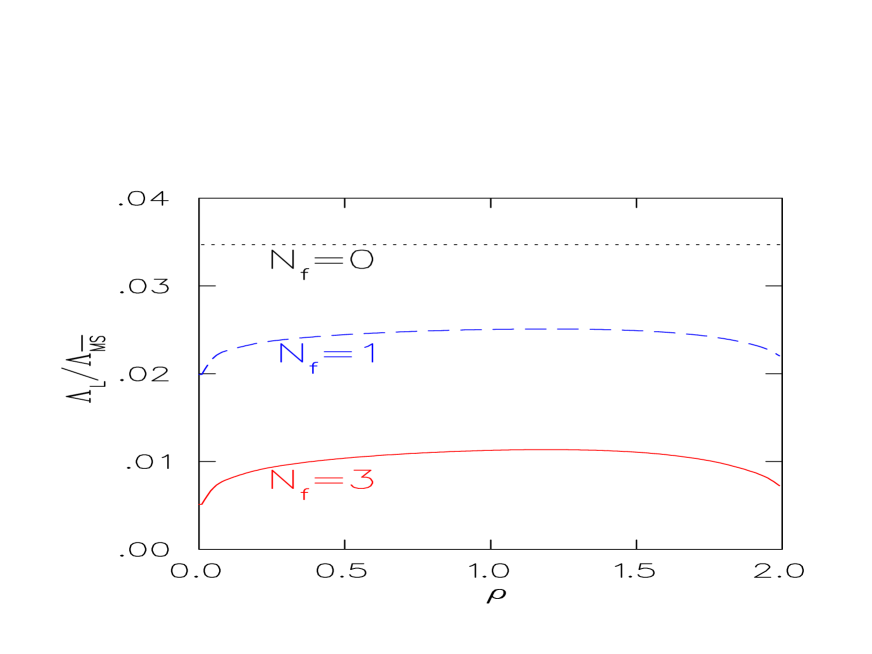
FIG. 2.: $\Lambda_{L}/\Lambda_{\overline{\rm MS}}$ in $SU(3)$, as a function of the parameter $\rho\,$. $N_{f}=0$ (dotted line), $N_{f}=1$ (dashed line), $N_{f}=3$ (solid line).

The coefficients $d_{n,i}$ obey two constraints, which we have used as verifications of our procedure:

• Gauge invariance requires $\sum_{i}d_{0,i}=0$. One may check this property both on the algebraic expressions and on the numerical results. Substituting the numerical results for the coefficients, we find zero within the error estimates, for all values of $\rho\,$; this serves also to verify our estimation of systematic errors.

• The coefficients $d_{2,i}$ must coincide with those of the continuum. We checked that this is so: $d_{2,1}={2/3}\,,\ d_{2,2}=0\,.$

Thus, our result takes the form

$$\nu^{(1)}(ap)\mid_{\lambda_{0}=1}=\nu^{(1)}(ap)\mid_{N_{f}=0,\;\lambda_{0}=1}+N_{f}\left[{1\over 24\pi^{2}}\ln(a^{2}p^{2})+k_{f}(\rho)\right],$$ (40)

where

$$\nu^{(1)}(ap)\mid_{N_{f}=0,\;\lambda_{0}=1}=-{11N\over 48\pi^{2}}\ln(a^{2}p^{2})-{1\over 8N}+0.21709849N$$ (41)

is the pure gauge part [34, 35, 30], and $k_{f}(\rho)=d_{1,1}+d_{1,2}\,$ is presented in Table 1. We note again that the choice of the pure gluonic part of the action affects the first, but not the second, summand in Eq. (40).

From Eqs. (14, 18, 21), we find

$$l_{0}={1\over 8N}-0.16995599N+N_{f}\left[-{5\over 72\pi^{2}}-k_{f}(\rho)\right].$$ (42)

The values of $\Lambda_{L}/\Lambda_{\overline{\rm MS}}$ follow immediately from Eq. (15). Some particular cases of interest are ($N=3$):

$$\Lambda_{L}/\Lambda_{\overline{\rm MS}}\bigr{|}_{N_{f}{=}0}=0.034711$$ (43)

$$\Lambda_{L}/\Lambda_{\overline{\rm MS}}\bigr{|}_{N_{f}{=}1,\ \rho{=}1}=0.025042$$ (44)

$$\Lambda_{L}/\Lambda_{\overline{\rm MS}}\bigr{|}_{N_{f}{=}3,\ \rho{=}1}=0.011273$$ (45)

For comparison we report the corresponding values of the ratio $\Lambda_{L}/\Lambda_{\overline{\rm MS}}$ for the standard Wilson formulation of fermions [36]

$$\Lambda_{L}/\Lambda_{\overline{\rm MS}}\bigr{|}_{N_{f}{=}1,\ r{=}1}=0.029412$$ (46)

$$\Lambda_{L}/\Lambda_{\overline{\rm MS}}\bigr{|}_{N_{f}{=}3,\ r{=}1}=0.019618.$$ (47)

Acknowledgements: H. P. would like to acknowledge the warm hospitality extended to him by the Theory Group in Pisa during various stages of this work.

REFERENCES

- [1] H. Neuberger, Phys. Lett. B 417 (1998) 141; B 427 (1998) 353.
- [2] R. Narayanan and H. Neuberger, Nucl. Phys. B 443 (1995) 305.
- [3] H. B. Nielsen and M. Ninomiya, Phys. Lett. B 105 (1981) 219; Nucl. Phys. B 185 (1981) 20; erratum Nucl. Phys. B 195 (1982) 541.
- [4] H. Neuberger, “The overlap lattice Dirac operator and dynamical fermions”, hep-lat/9901003.
- [5] P. Hernández, K. Jansen, and M. Lüscher, Nucl. Phys. B 552 (1999) 363.
- [6] P. H. Ginsparg and K. G. Wilson, Phys. Rev. D 25 (1982) 2649.
- [7] P. Hasenfratz, Nucl. Phys. B 525 (1998) 401.
- [8] S. Chandrasekharan, “Lattice QCD with Ginsparg-Wilson fermions”, hep-lat/9805015, Phys. Rev. D, in press.
- [9] Y. Kikukawa and A. Yamada, Nucl. Phys. B 547 (1999) 413.
- [10] M. Lüscher, Phys. Lett. B 428 (1998) 342.
- [11] M. Lüscher, Nucl. Phys. B 538 (1999) 515.
- [12] T.-W. Chiu, Phys. Lett. B 445 (1999) 371.
- [13] K. Fujikawa, Nucl. Phys. B 546 (1999) 480.
- [14] H. Suzuki, “Simple evaluation of the chiral Jacobian with the overlap Dirac operator”, hep-th/9812019, Prog. Theor. Phys., in press.
- [15] D. H. Adams, “Overlap topological charge and axial anomaly for lattice fermions with overlap-Dirac operator”, hep-lat/9812003.
- [16] T. Reisz and H. J. Rothe, “Renormalization of lattice gauge theories with massless Ginsparg Wilson fermions”, hep-lat/9908013.
- [17] H. Neuberger, Phys. Rev. Lett. 81 (1998) 4060.
- [18] R. G. Edwards, U. M. Heller, and R. Narayanan, Nucl. Phys. B 540 (1999) 457.
- [19] R. G. Edwards, U. M. Heller, and R. Narayanan, Phys. Rev. D 59 (1999) 094510.
- [20] H. Neuberger, “Minimizing storage in implementations of the overlap lattice-Dirac operator”, hep-lat/9811019.
- [21] R. G. Edwards, U. M. Heller, and R. Narayanan, “Chiral fermions on the lattice”, hep-lat/9905028.
- [22] L. Giusti, Ch. Hoelbling, and C. Rebbi, “Considerations on Neuberger’s operator”, hep-lat/9906004.
- [23] P. Hernández, K. Jansen, and L. Lellouch, “Finite-size scaling of the quark condensate in quenched lattice QCD”, hep-lat/9907022.
- [24] UKQCD Collaboration, C. McNeile, A. Irving, and C. Michael, “Feasibility study of using the overlap-Dirac operator for hadron”, hep-lat/9909059.
- [25] K. F. Liu, S. J. Dong, F. X. Lee, and J. B. Zhang, “Hadron masses and quark condensate from overlap fermions”, hep-lat/9909061.
- [26] H. Neuberger, Phys. Rev. D 57 (1998) 5417.
- [27] L. F. Abbott, Nucl. Phys. B 185 (1981) 189.
- [28] R. Dashen and D. J. Gross, Phys. Rev. D 23 (1981) 2340.
- [29] M. Lüscher and P. Weisz, Nucl. Phys. B 452 (1995) 213.
- [30] M. Lüscher and P. Weisz, Nucl. Phys. B 452 (1995) 234.
- [31] C. Christou, A. Feo, H. Panagopoulos, and E. Vicari, Nucl. Phys. B 525 (1998) 387.
- [32] H. Panagopoulos, “The 3-loop -function of QCD in the clover formulation”, in preparation.
- [33] Y. Kikukawa and A. Yamada, Phys. Lett. B 448 (1999) 265.
- [34] A. Hasenfratz and P. Hasenfratz, Nucl. Phys. B 193 (1981) 210.
- [35] A. Gonzales-Arroyo and C. P. Korthals Altes, Nucl. Phys. B 205 (1982) 46.
- [36] H. Kawai, R. Nakayama and K. Seo, Nucl. Phys. B 189 (1981) 40.