Review on string breaking
– the query in quest of the evidence –

Abstract

Considerable progress has been achieved recently in the observation of string breaking within non-Abelian Higgs models, by use of multi-channel methods allowing for broken string states. Similarly, in pure gauge theory this approach has been shown to reveal string breaking for color charges in the adjoint represenation. For QCD with dynamical fermions, one needs substantial progress in noise reduction, however, to render such techniques viable.

1 INTRODUCTION

Twenty years after the demonstration of confinement in quenched QCD simulations [1] we have beautiful evidence of the formation of colour flux tubes between static colour charges [2]. As to the verification of their fission, it has been anticipated ever since that full QCD calculations should reveal string breaking (SB), in form of a screening behaviour in the static potential $V(R)$.

While studies on Polyakov loop correlators in the temperature range $.68\leq T/T_{c}\leq.94$ [3] reviewed at LATTICE98 [4] did indeed provide clear evidence for such phenomenon (cf. also the arguments presented in [5]), the head-on approach for detection of SB signals from mere Wilson loop studies at $T=0$ has not proven successful [6]. This situation is illustrated in Fig. 1 e.g., with updated T$\chi$L data [7].

But why bother about SB if one expects it anyhow? The motivations to focus on the challenge are obvious: (a) the $R$-asymptotia of $V(R)$ is the most obvious infrared quantity that we can target on the lattice and hence important to be under control, (b) SB can teach us both about the techniques to handle mixing problems and hadron decays like $\Upsilon\rightarrow B\bar{B}$ on the lattice [9]. Lastly, understanding hadronization in the static interaction scenario of full QCD will certainly help to further substantiate previous quenched results on confinement [10]. For we should remember that transfer matrix studies yield at best numerical estimates of

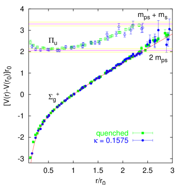
Figure 1: Update of full QCD potential from T$\chi$L (at $\beta=5.6$) [7], in comparison to their quenched result at $\beta_{q}=6.0$, with Sommer radius $r_{0}$ [8].

upper bounds to $V$ as long as we are analyzing asymptotic (in Euclidean time $T$) behaviour of Wilson loops $W$ in terms of $dlnW(R,T)/dT\rightarrow-V(R)$, at finite $T$.

2 VISIBILITY: 5 LATTICE SPACINGS

Quenched analyses of static potentials rely – apart from high statistics – on the combined action of three signal enhancing techniques : (a) smearing the spatial links in order to suppress excited state contaminations, (b) analytic multihit noise reduction on the time-like links, (c) exploiting loop averaging effects on each configuration by shifting and measuring $W$ all over the entire lattice.

In full QCD we are in lack of high statistics samples of vacuum configurations (for cost reasons) and moreover, we have to abandon multihitting as it becomes unfeasable in presence of long range quark loop effects. In Fig.2 I demonstrate the quality of the resulting plateau in the effective potential, $V_{eff}(2.4r_{0},T)$. Evidently, one runs into rapidly increasing errors when going beyond $T=5-6$!

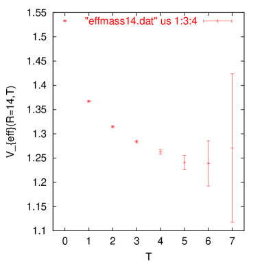
Figure 2: Plateau formation in $V_{eff}(2.4r_{0})$ at $\beta=5.6$ and $\kappa_{sea}=.1575$, from T$\chi$L configs. [7]

The lesson to be learnt from Fig.2 is obviously that – in order to uncover SB – one better aims at achieving an improved overlap with the true ground state [11], in terms of an earlier onset of the plateau, in a region where the resolution of the effective potential still suffices, at time separations $3,4,$ and $5$.

Let me just mention in passing an alternative strategy to establish SB: (a) determine in full QCD the masses of torelons, i.e. the spatial wrappers (of length $L$) around the lattice [12]; (b) compute an effective string tension, $K$, like in quenched QCD from a fit to the potential at $r<2r_{0}$ where string breaking is not yet expected to set in; (c) torelon effective masses undershooting the string energy would provide evidence for SB. As illustrated in Fig. 3 the SESAM data on the $16^{3}\times 32$ lattice at their smallest quark mass exhibits some weak evidence for SB, by crossing the level $\sigma L=16K$, though at rather high noise level.

Another aspect which has been brought forward recently [13] is to exploit coarse grained spatial lattices by help of improved actions.

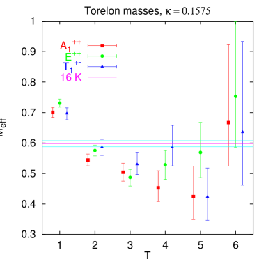
Figure 3: Effective torrelon masses from SESAM configurations at $\kappa_{sea}=.1575$ [14].

3 MULTICHANNEL APPROACH

The obvious strategy for improving the ground state overlap is to enlarge the operator space to a multichannel approach comprising

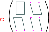
Figure 4: The two channel transfer matrix $C(T)$ in the non-Abelian Higgs model, with due tribute to Pisa: the bullets stand for scalar mass insertions.

hadronization. This would be very much in the spirit of multi-operator variational ansätze as devised and used largely in the context of glueball studies. In the present context strong coupling methods have been used to demonstrate [15] that inclusion of the $Q\bar{Q}$ $q\bar{q}$ channel in addition to the static quark-antiquark $Q\bar{Q}$ (with fluxtube in between) looks like a promising path for uncovering SB. It implies however the use of large loops with color partly transmitted by insertion of light quark propagators (instead of by gauge links only).

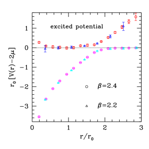
Figure 5: Scaling of ground and excited states potential in the SU(2) Higgs model [20].

This feature precludes us from applying easy loop averaging over the entire lattice, since light quark propagators are too expensive to compute for all source points on the lattice.

4 SB WITHOUT FERMIONS

Given the problems to deal with fermions refs. [16, 17] followed an old suggestion of Bock et al [18] to study the mechanism of SB in an easier setting, namely by resorting to non-Abelian Higgs fields.

In the two-channel scenario (see Fig. 4) one is faced with a generalized eigenvalue problem of the transfer matrix, for evolution from $T_{0}=0$ to $T$ , with eigenvalues $\lambda_{i}(T,T_{0})$ [19]

$$C(T)\;\vec{c}_{i}=\lambda_{i}(T,T_{0})\quad C(T_{0})\;\vec{c}_{i},$$ (1)

the index labeling ground ($i=0$) and excited state ($i=1$). In a contribution to this conference Knechtli et al [20] have presented a high statistics scaling study of an SU(2) Higgs model in 3+1 dimensions, with matter field $\Phi$ in the fundamental representation, in the confining phase. As can be seen from Fig. 5 they can neatly trace both ground and excited states in a scaling regime, with a clear-cut gap in between.

Moreover they show that the overlap function of the Wilson loop operator to the true ground state, $\omega_{0}^{W}(R)$, computed according to

$$\Omega(T)=(\vec{c}_{0},C(T)\;\vec{c}_{0})=\sum_{n}\omega_{n}\exp{(-V_{n}T)},$$ (2)

with $\Omega(0)=1$ exhibits a steeply falling $R$-dependence, as shown in Fig. 6. They illustrate moreover that a naive one-channel analysis is manifestly misleading, as it yields an overlap estimate, $\omega^{W,naive}_{0}$, that fakes a good projection of the large Wilson loops to the ground state!!

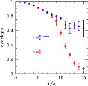
Figure 6: The overlap of the Wilson loop operator, $\omega_{0}$, with the broken string ground state [20].

As yet another check for the efficiency of the two-channel approach in revealing SB, two detailed studies [21, 22] were addressed recently to the adjoint flux tube formation between static color charges in the adjoint representation of SU(2) gauge theory in 2+1 dimensions. Such strings are not protected from breaking up, even in absence of fermions [23]. In the correlation matrix $C$ (see Fig 4) the mass insertions are now to be replaced by gluelump operators[24], $\mbox{gluelump}_{a}^{x}=Tr\big{(}\mbox{clover}_{a}^{x}\sigma_{a}\big{)}$ (with color $a$ and site $x$) to be linked by the color flux operator $Tr\big{(}\sigma^{a}\;U_{x\rightarrow y}\;\sigma^{b}\;U^{\dagger}_{x\rightarrow y}\big{)}$. Fig. 8 highlights beautifully the efficiency of the multichannel ansatz in revealing, in addition to the ground state, another three excited states, along with resolution of their level crossings!

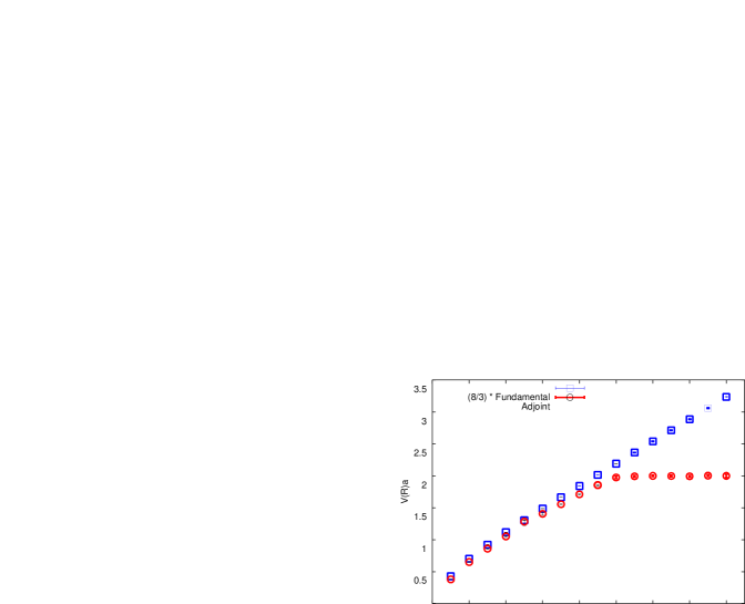
Figure 7: SB in adjoint potential compared to confinement in static potential in fundamental representation in 2+1d SU(2) g.t., from ref. [22].

Figure 8: SB observed for three different excitation levels of the adjoint string, from ref. [21].

Having convinced ourselves that an operator set extended to include physically motivated channel mixing is the right way to go, let us return to our original problem, i.e. QCD with fermions.

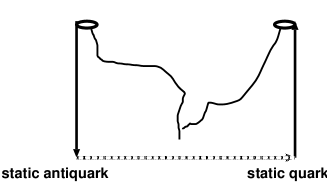
Figure 9: Transition matrix element from state $Q\bar{Q}$ to state $Q\bar{Q}$ $q\bar{q}$ , with source/sink smearing.

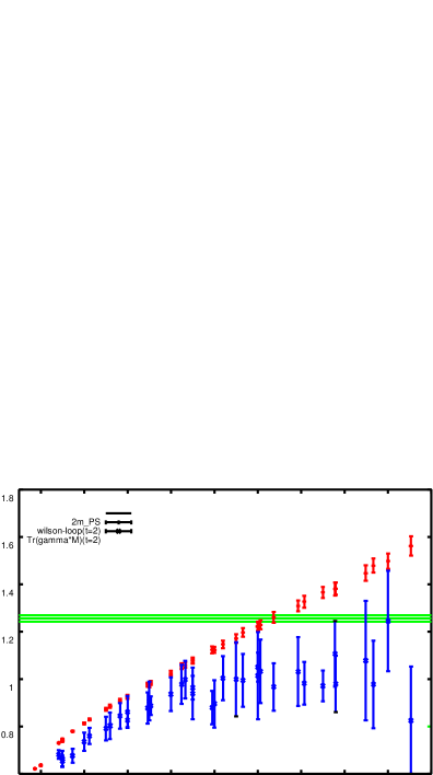
Figure 10: Noise on local masses vs $R$, at $T=2$: small (large) error points refer to Wilson loops (transition matrix elements, $\langle 2|C|1\rangle$, cf. Fig. 9); horizontal lines mark the error band for $2m_{PS}$. Analysis done on T$\chi$L configs, at $\kappa_{sea}=.1575$ and $r_{0}\approx 5.9a$ [25].

5 UNCOVER SB IN QCD?

If we wish to adopt the multichannel strategy to the QCD situation, we have to deal with loops containing insertion of light quark propagators, like in the transition correlator $\langle 2|C|1\rangle$ depicted in Fig. 9.

Fig. 10 [25] illustrates the noise situation with the example of local masses from the transition correlator, $\langle 2|C|1\rangle$. While source smearing helps a lot, doing without loop averaging makes things hopeless, even at a small value of $T$, such as $T=2(!)$. This can best be seen by comparing to the noise level in the corresponding Wilson loop, $\langle 1|C|1\rangle$! One should be aware that the noise situation is considerably aggravated for $\langle 2|C|2\rangle$, at $T=3$ or $4$! Similar observations have been reported by Lacock for the MILC collaboration [26].

In order to get noise under control one obviously needs the computation of light quark propagators $P(x\rightarrow y)=M^{-1}_{xy}$ on source locations sampled over a large region, $R$, of the lattice volume. A promising program in this direction has been launched recently by Michael et al.[27] Their proposal is to start out from a Gaussian estimate for inverse Dirac operator in terms of a random scalar field $\Phi$.

$$M^{-1}_{xy}=\frac{1}{Z}\int D\Phi\quad\Phi_{y}^{*}\Phi_{x}\exp{\{-\Phi^{*}M\Phi/2\}}\quad.$$ (3)

The estimator introduces additional noise whose variance can be minimized by a multihit (analytical integration) on $\Phi$ over the interior region of $R$, $I=R-\partial R$. In praxi, this requires computation of an inverse block matrix $\bar{M}^{-1}$ (by iterative solver) after each update of the $\Phi$-field on the boundary $\partial R$, as borne out in the replacement:

$$\Phi_{x}\rightarrow v_{x} = \int_{\Phi\subset I}D\Phi\quad\Phi_{z}\exp{\{-\Phi^{*}M\Phi/2\}}$$ (4)

$$= -\bar{M}^{-1}_{xx^{\prime}}\tilde{M}_{x^{\prime}z}\Phi_{z}\quad.$$

Here $\bar{M}$ ($\tilde{M}$) is a block matrix with support $\subset I=R-\partial R$ ($R$) and $z\in\partial R$ .

So far this noise reduction technique has been applied successfully to the determination of forces between two static-light mesons [28]. It remains to be seen whether it can bring decisive progress in the treatment of QCD string fission.

6 PISA EST OMEN?

While in confining models without fermions, SB has been clearly seen at work, we have at this stage no real compelling evidence for string breaking from simulation of QCD with dynamical fermions.

In any case, from meditating on Fig. 11 which is a zoom to this years conference poster a superstitious person might suppose that at present Pisa would not offer favourable auspices for the occurence of string breaking.

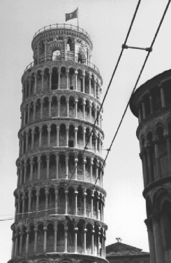
Figure 11: The Pisa model for b-confinement.

So for the time being, let me finish by quoting a famous last century tourist who felt frustration after climbing (the tower?): “Spitze Steine – Müde Beine – Aussicht keine – Heinrich Heine”. What about Heine being wrong?

Acknowledgements

My great thanks to the organizers for the superb conference. I enjoyed interesting discussions with G. Bali, M. Peardon, and T. Struckmann during the preparation of this talk. I am grateful to G. Bali for his help in improving the manuscript.

References

- [1] M. Creutz, Phys. Rev. D21 (1980) 2308.
-
[2]
http://www.theorie.physik.uni-wuppertal.de/comphys/Dokumente/Femtowelt
/welcome.phtml.de - [3] E. Laermann et al., PR D59 (1999) 031501; for earlier related work, see M.E. Faber et al., Phys. Lett B200 (1988) 348; W. Bürger et al., Phys. Rev. D47 (1993) 3034.
- [4] J. Kuti, Nucl. Phys. Proc. Suppl. 73 (1999) 72.
- [5] F. Gliozzi et al., these proceddings.
- [6] U. Glässner et al., Phys. Lett. B383 (1996) 98; M. Talevi et al, Nucl. Phys. Proc. Suppl. 63 (1998) 227; S. Aoki et al, hep-lat/9902018.
- [7] G.S. Bali, B. Bolder, private communication.
- [8] R. Sommer, Nucl. Phys. B411 (1994) 839.
- [9] I.T Drummond, Phys. Lett, B447 (1999)298.
- [10] G.S. Bali et al. Phys. Rev. D47 (1993) 661.
- [11] S. Güsken, Nucl. Phys. Proc. Suppl. 63 (1998) 209.
- [12] C. Michael, Phys. Lett. B232 (1989) 232.
- [13] H.D. Trottier, Phys. Rev. D60 (1999) 034506.
- [14] G.S. Bali, private communication.
- [15] I.T. Drummond, Phys. Lett. B442 (1998) 279.
- [16] F. Knechtli et al., Phys. Lett. B440 (1998) 345.
- [17] O. Philipsen et al., Phys. Rev. Lett. 81 (1998) 4056.
- [18] W. Bock et al., Z. Phys. C45 (1990) 597.
- [19] M. Lüscher et al., Nucl. Phys. B339 (1990) 222.
- [20] F. Knechtli, these proceedings.
- [21] O. Philipsen, H. Wittig, Phys. Lett. B451 (1999) 146.
- [22] P. Stephenson, Nucl. Phys. B550(1999)427.
- [23] C. Michael, Nucl. Phys. Proc. Suppl. 26 (1992) 417.
- [24] L.A. Griffiths et al., Phys. Lett. B129 (1983) 351.
- [25] T. Struckmann, private communication.
- [26] P. Lacock, these proceedings.
- [27] C. Michael et al. Phys. Rev. D58 (1998) 034506.
- [28] C.Michael et al., Phys. Rev. D60 (1999) 054012.