The second moment of the pion’s distribution amplitude

Abstract

We present preliminary results for the second moment of the pion’s distribution amplitude. The lattice formulation and the phenomenological implications are briefly reviewed, with special emphasis on some subtleties that arise when the Lorentz group is replaced by the hypercubic group. Having analysed more than half of the available configurations, the result obtained is $\langle\xi^{2}\rangle_{L}=0.06\pm 0.02$.

1 INTRODUCTION

The distribution amplitude $\phi(x_{1},x_{2})$ gives the probability for finding two collinear partons with fractions $x_{1}$ and $x_{2}$ of the meson’s momentum [1]. It plays an important role e.g. in exclusive hard scattering processes and in non-leptonic decays of heavy mesons, since it allows one to separate a hard scattering amplitude, computed in perturbation theory, from the effect of the soft Fourier modes, whose dynamics is non-perturbative.

For example, the relevant diagram for the pion electromagnetic form factor is shown in Fig. 1. The form factor is defined as:

$$\langle\pi(p^{\prime})|V_{\mu}|\pi(p)\rangle=F(q^{2})(p+p^{\prime})_{\mu}$$ (1)

and can be written in terms of the distribution amplitude:

$$F(Q^{2})=$$ (2)

$$\int[{\mathrm{d}}x][{\mathrm{d}}y]\>\phi^{\dagger}(x,Q^{2})T_{H}(x,y;Q^{2})\phi(y,Q^{2})$$

where $[{\mathrm{d}}x]={\mathrm{d}}x_{1}{\mathrm{d}}x_{2}\delta(x_{1}+x_{2}-1)$, and $T_{H}$ is the perturbative amplitude computed at the quark level.

Figure 1: Photon-pion interaction, factorised into a hard (perturbative) scattering amplitude and a non-perturbative part described by the pion distribution amplitude.

The amplitude $\phi$ is given by the non-local Fourier transform of the matrix element of the fermionic bilinear [2]:

$$\phi^{ab}_{\alpha\beta}(x,Q^{2})\sim FT\left[\langle 0|T\psi^{a}_{\alpha}(z_{1})\bar{\psi}^{b}_{\beta}(z_{2})|\pi\rangle\right]$$ (3)

A light-cone expansion relates $\phi$ to fermion bilinears with covariant derivatives. In particular the $m$-th moment,

$$\langle\xi^{m}\rangle\equiv\int{\mathrm{d}}\xi\>\xi^{m}\phi(\xi,Q^{2}),$$ (4)

can be extracted from the matrix element of the lowest-twist operator appearing in the OPE of Eq. 3:

$$\langle 0|O_{\mu_{0}\ldots\mu_{m}}(0)|\pi(p)\rangle=f_{\pi}\>p_{\mu_{0}}\ldots p_{\mu_{m}}\>\langle\xi^{m}\rangle+\cdots$$ (5)

where

$$O_{\mu_{0}\ldots\mu_{m}}(0)=(-i)^{n}\bar{\psi}\>\gamma_{\mu_{0}}\gamma_{5}\>\stackrel{{\scriptstyle\leftrightarrow}}{{D}}_{\mu_{1}}\ldots\stackrel{{\scriptstyle\leftrightarrow}}{{D}}_{\mu_{m}}\psi$$ (6)

and the ellipses indicate terms that are proportional to $p^{2}g_{\mu_{i}\mu_{j}}$.

The distribution amplitude has been studied in recent years using sum rules (see results quoted in [1]) and lattice simulations [3, 4]. The accuracy of the lattice determinations so far has not been good enough to compare precisely with sum rules predictions. The aim of the current study is to use modern lattice technology to improve the precision of the result.

2 LATTICE DETAILS

The following UKQCD quenched configurations have been used to compute the relevant matrix elements.

• $\beta=6.2$, $a^{-1}=2.64\pm 0.10~{}\mbox{GeV}$, $24^{3}\times 48$ lattice;

• SW action, with $c_{\mathrm{sw}}=1.61$;

• the three $\kappa$ values used in our simulation (0.13460, 0.13510, 0.13530) correspond to physical light pseudoscalar masses ranging from 350 to 850 MeV.

• 180 configurations are available, the results presented here are based on the analysis of a subset of 129;

• non-improved local operators have been used, without fuzzing of the light quarks.

3 POWER-LIKE DIVERGENCIES

In this work, we concentrate on the second moment of the distribution amplitude, i.e. $m=2$ in Eq. 5 and 6 above. The choice of the Lorentz indices for $O_{\mu_{0}\mu_{1}\mu_{2}}$ is crucial in order to avoid mixing with lower-dimensional operators. We choose $\mu_{0}$ to be the time-direction. It is convenient, but not necessary, to avoid time-derivatives and hence we do not symmetrise $\mu_{0}$ with $\mu_{1},\mu_{2}$. Using the notation of [5] to classify the irreducible representations of the hypercubic group, we obtain:

• $O_{\mu[\nu\sigma]}$, with $\mu\!\neq\!\nu\!\neq\!\sigma\!\neq\!\mu$ and symmetrised over $\nu$ and $\sigma$, transforms like a $\overline{(\frac{1}{2},\frac{1}{2})}\oplus\mathbf{8}$ reducible representation, and therefore does not mix with lower dimensional operators. However the $\mathbf{8}$ irrep leads to a term proportional to $p_{\mu}\left[\frac{p_{\nu}^{2}+p_{\sigma}^{2}}{2}-p_{\tau}^{2}\right]$, where $\tau$ is the fourth available index, which needs to be subtracted in order to have an operator proportional to $p_{\mu}p_{\nu}p_{\sigma}$, as in the continuum limit. This subtraction is performed in the definition of $R_{1}$ below. Note that two spatial components of $p$ need to be non-zero to get a non-vanishing signal.

• $O_{\mu\nu\nu}$, with $\mu\!\neq\!\nu$ transforms like a $(\frac{1}{2},\frac{1}{2})\oplus\mathbf{8}$ representation; however the subtracted operator:

  $$O_{411}^{\prime}=\left(O_{411}-\frac{O_{422}+O_{433}}{2}\right)$$

  simply transforms like $\mathbf{8}$. In this case there is no mixing, and a non-zero signal is obtained with just one non-vanishing component of $p=(1,0,0)$.

4 PRELIMINARY RESULTS

The relevant matrix elements are extracted from suitably defined two-point functions. For a generic operator $Q$:

$$C_{2}^{Q}(t) = \sum_{\mathbf{x}}e^{i\mathbf{p}\mathbf{x}}\langle Q(\mathbf{x},t)\>\bar{\psi}\gamma_{5}\psi(0)\rangle$$ (7)

$$\stackrel{{\scriptstyle t\rightarrow\infty}}{{\rightarrow}} \frac{Z}{2E}\>\langle 0|Q(0)|\pi(p)\rangle\>e^{-Et}$$

where $Z=\langle\pi(p)|\bar{\psi}\gamma_{5}\psi(0)|0\rangle$.

For large time separations:

$$R_{1} = \left.\frac{C_{2}^{O}(t)}{C_{2}^{A}(t)}\right|_{\mathbf{p}=(1,1,0)}-\left.\frac{C_{2}^{O}(t)}{C_{2}^{A}(t)}\right|_{\mathbf{p}=(1,0,0)}$$

$$= p_{1}\,p_{2}\langle\>\xi^{2}\rangle$$

$$R_{2} = {C_{2}^{O^{\prime}}(t)}/{C_{2}^{A}(t)}$$

$$= p_{1}^{2}\>\langle\xi^{2}\rangle$$

Only the results for the heavier $\kappa$ are presented here. The pion propagator is shown in Fig. 2. The effective mass and single-exponential fits give consistent results for $6<t<15$. Since the relative error on the signal of interest for the second moment becomes large for $t>15$, the fitting ranges chosen in this work are shorter than the ones usually used for light spectroscopy. Despite this discrepancy, our value for $f_{\pi}$ agrees with other UKQCD determinations from the same set of configurations within $2\sigma$.

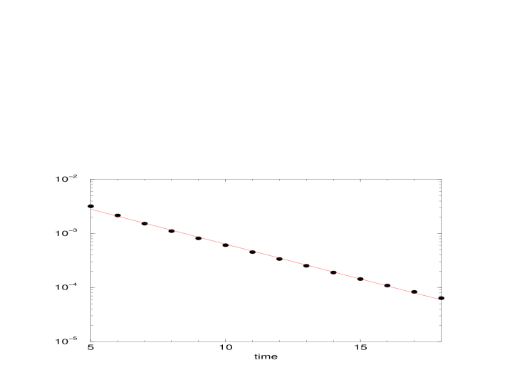
Figure 2: Pion propagator from 129 configurations at $\kappa=0.13460$

The time dependence of $R_{2}$, obtained from 129 configurations, is given in Fig. 3. We have currently analysed $R_{1}$ on 55 configurations only. In order to compare the two determinations, the results for $R_{1}$ are also displayed in the same figure. The agreement between the two sets of results is good. At this preliminary stage $R_{2}$ alone is used to extract our final number.

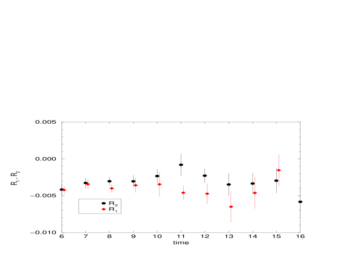
Figure 3: Ratios of two-point functions $R_{1}$ and $R_{2}$ for $\kappa=0.13460$. The results for $R_{1}$ and $R_{2}$ are obtained from 55 and 129 configurations respectively.

5 CONCLUSIONS

Fitting the points in Fig. 3 to a constant yields

$$\langle\xi^{2}\rangle_{L}=0.06\pm 0.02$$

for the lattice value of the second moment of the pion distribution amplitude. The analysis of the complete set of available configurations for both $R_{1}$ and $R_{2}$, together with a full discussion of the systematic errors, will be presented in a forthcoming publication [6]. The statistical error in our result will of course decrease as the number of configurations is increased. The multiplicative renormalisation of the operator has yet to be calculated, either perturbatively or non-perturbatively.

Our preliminary result for the value of $\langle\xi^{2}\rangle$ suggests that it is lower than the value predicted by sum rules. Such a result could be explained for example by a more peaked distribution for $\xi$ around the origin.

Computations of the distribution amplitudes of the $\rho$ meson and the proton are currently under way. Our analysis can also be extended to the case of non-degenerate quarks and so a study of the distribution amplitudes of the $K$ and $B$ mesons is feasible.

References

- [1] for a review and extensive references, see V.L. Chernyak, I.R. Zhitnitsky, Phys. Rep. 112 (1984) 173
- [2] S. Brodsky et al., Phys. Lett. 91 B (1980) 239
- [3] G. Martinelli and C. Sachrajda, Phys. Lett. B 190 (1987) 151
- [4] T. Daniel, R. Gupta, D. Richards, Phys. Rev. D 43 3715 (1991)
- [5] J. Mandula, G. Zweig, J. Govaerts, Nucl. Phys. B 228 (1980) 91
- [6] L. Del Debbio, M. Di Pierro, A. Dougall, C.T. Sachrajda, in preparation