Calculation Of Hadronic Matrix Elements Relevant For $\Delta I=1/2$ Rule And $\varepsilon^{\prime}/\varepsilon$ In Lattice QCD With Staggered Fermions

Abstract

This thesis presents the setup and results of numerical calculation of hadronic matrix elements of $\Delta S=1$ weak operators, with the aim of studying the $\Delta I=1/2$ rule and direct CP violation. Such study provides a useful comparison of the Standard Model predictions with experiment. We work within the framework of (partially quenched) Lattice QCD with the staggered (Kogut-Susskind) version of fermions. We have achieved a reasonable statistical accuracy in calculating all matrix elements in question. Based on these results, we find that the $\Delta I=1/2$ channel in $K\to\pi\pi$ decays is enhanced compared to the $\Delta I=3/2$ channel. This is consistent with experiment, although the exact amount of enhancement is subject to considerable systematic errors. I also discuss the difficulties encountered in attempting to calculate the direct CP violation parameter $\varepsilon^{\prime}/\varepsilon$ and our approximate solution leading to a crude estimate. In a related study we nonperturbatively compute bilinear renormalization factors $Z_{S}$ and $Z_{P}$, which are needed for our estimate of $\varepsilon^{\prime}/\varepsilon$ and also allow to calculate the light quark masses. For the strange quark mass in NDR $\overline{\rm MS}$ scheme at 2 GeV in the quenched approximation we find: $m_{s}=102.9\pm 5.1$ MeV.

This thesis presents the setup and results of numerical calculation of hadronic matrix elements of $\Delta S=1$ weak operators, with the aim of studying the $\Delta I=1/2$ rule and direct CP violation. Such study provides a useful comparison of the Standard Model predictions with experiment. We work within the framework of (partially quenched) Lattice QCD with the staggered (Kogut-Susskind) version of fermions. We have achieved a reasonable statistical accuracy in calculating all matrix elements in question. Based on these results, we find that the $\Delta I=1/2$ channel in $K\to\pi\pi$ decays is enhanced compared to the $\Delta I=3/2$ channel. This is consistent with experiment, although the exact amount of enhancement is subject to considerable systematic errors. I also discuss the difficulties encountered in attempting to calculate the direct CP violation parameter $\varepsilon^{\prime}/\varepsilon$ and our approximate solution leading to a crude estimate. In a related study we nonperturbatively compute bilinear renormalization factors $Z_{S}$ and $Z_{P}$, which are needed for our estimate of $\varepsilon^{\prime}/\varepsilon$ and also allow to calculate the light quark masses. For the strange quark mass in NDR $\overline{\rm MS}$ scheme at 2 GeV in the quenched approximation we find: $m_{s}=102.9\pm 5.1$ MeV.

To my parents

November 29, 1971Born - Kiev, Ukraine, USSR

1991B.S. equivalent, Physics, Moscow
Institute of Physics and Technology

1993-1995Graduate Teaching Associate,
Department of Physics,
The Ohio State University. 1995M.S., Physics,
The Ohio State Univerity 1995-presentGraduate Research Associate,
Department of Physics,
The Ohio State University.

D. Pekurovsky, G. Kilcup “Lattice Calculation of Matrix Elements Relevant For $\Delta I=1/2$ Rule and $\varepsilon^{\prime}/\varepsilon$” Published electronically by the library of UCLA at:
http://www.dpf99.library.ucla.edu

D. Pekurovsky, G. Kilcup “$\Delta I=1/2$ Rule from Staggered Fermions” Nucl. Phys. B (Proc. Suppl.) 73, 309–311 (1999)

D. Pekurovsky, G. Kilcup “Weak Matrix Elements: On the Way to $\Delta I=1/2$ rule and $\varepsilon^{\prime}/\varepsilon$ with staggered fermions” Nucl. Phys. B (Proc. Suppl.) 63, 293–295 (1998)

G. Kilcup, D. Pekurovsky, L. Venkataraman “On the $N_{f}$ and $a$ dependence of $B_{K}$” Nucl. Phys. B (Proc. Suppl.) 53, 345–348 (1997)

Physics

Lattice QCDProf. G. Kilcup

Chapter 1 Introduction

1.1 Overview

One of the main directions of efforts in both experimental and theoretical particle physics is obtaining reliable information about the fundamental free parameters of the Standard Model (SM). These parameters include the masses of quarks, leptons, $W$ and $Z$ gauge bosons, and the Higgs particle; coupling constants of electroweak and strong interactions; and the elements of the Cabibbo-Kobayashi-Maskawa (CKM) matrix. Without the exact knowledge of all of these parameters, the SM lacks the full predictive power. Such knowledge would also allow to perform various consistency checks based on results of independent experiments. In addition, there is another important reason for knowing the SM parameters: many alternative theories of fundamental particle interactions have been proposed. Among such theories are various extensions of the SM, as well as Supersymmetric Grand Unified Theories (SUSY GUTs), in which the SM itself is a low-energy limit of more fundamental and unifying theories. In order to check if extensions of SM are really necessary and to check if any of the proposed alternatives to the SM are indeed valid descriptions of physical reality, it is necessary to know the parameters of the SM.

In many cases obtaining the SM parameters from experiment is difficult or impossible due to the presence of non-perturbative effects. For example, in order to extract certain CKM matrix elements, very often it is necessary to calculate matrix elements (MEs) of weak interaction operators between strongly interacting states (hadrons). In these cases the weak and strong interactions are tightly intertwined; hence there is an obligatory non-perturbative component in computing MEs, since the energy scales involved fall within the nonperturbative region of Quantum Chromodynamics (QCD), the theory of strong interactions. In calculating this nonperturbative component, as in other aspects of nonperturbative calculations in particle physics, Lattice Gauge Theory (LGT) plays an increasingly significant role. It is a first-principles method, and although several types of errors are inevitably introduced by lattice computations, rapid advances in available computational power as well as algorithmic techniques are allowing for steadily better control of such errors.

This thesis deals with several cases of application of Lattice QCD (LQCD) to calculating hadronic matrix elements of weak operators with the purpose of bridging the gap between theory and experiment and fixing the parameters of the SM. In addition, such calculations are aimed at testing nonperturbative QCD calculations against experiment so that the developed machinery of lattice calculations can be employed with confidence in other useful applications.

This work addresses the rich phenomenology of $K^{0}\to\pi\pi$ decays. One of the long-standing puzzles is the “$\Delta I=1/2$ rule”, which is the observation that the transition channel with isospin changing by 1/2 is enhanced 22 times with respect to transitions with isospin changing by 3/2. Weak interactions and the short-distance part of strong interactions are not enough to explain this phenomenon. In order to study the long-distance part of strong interactions (namely, to calculate hadronic matrix elements of the operators appearing in the effective weak Hamiltonian) a non-perturbative method has to be employed. In the work of this thesis, LQCD is used to this purpose. The aim is to explain the $\Delta I=1/2$ rule and to check the validity of several SM assertions used in obtaining the explanation, as well as to test the technology of lattice calculations.

In addition, I address the somewhat related issue of $\varepsilon^{\prime}$, the direct CP violation parameter in the neutral kaon system. Experimentally, the value of $\varepsilon^{\prime}/\varepsilon$ is measured to be non-zero. Resolving a 6 years old controversy, the Fermilab KTeV group [1] has recently announced their new measurement of $\mbox{Re}\,(\varepsilon^{\prime}/\varepsilon)$ at $(28.0\pm 4.1)\cdot 10^{-4}$. This is consistent with the latest reports from CERN group NA48 [2] of $\mbox{Re}\,(\varepsilon^{\prime}/\varepsilon)=(18.5\pm 7.3)\cdot 10^{-4}$ as well as with the value of $\mbox{Re}\,(\varepsilon^{\prime}/\varepsilon)=(23.0\pm 6.5)\cdot 10^{-4}$ measured by the CERN’s previous experiment NA31 [3]. Both Fermilab and CERN groups are currently analyzing their data, so enhanced statistics will soon allow to decrease the above errors. In addition, an experiment at Frascati is soon expected to measure the value of $\mbox{Re}\,(\varepsilon^{\prime}/\varepsilon)$ by a different technique.

It is clearly very interesting to compare the theoretical prediction for $\varepsilon^{\prime}/\varepsilon$ with the experimental result. Such a comparison will directly show if the minimal version of the SM correctly accounts for direct CP violation. Estimating $\varepsilon^{\prime}/\varepsilon$ is currently an area of considerable effort in the theoretical physics community [4]. According to some current estimates [5], it appears unlikely that the SM description of direct CP violation is correct, so that some extension or modification of the SM may be necessary. The weakest part of such estimates is the lack of knowledge of MEs of certain weak operators [6], which require nonperturbative treatment. In this work, LQCD is used for calculation of the relevant MEs.

The core of our work is calculation of matrix elements $\langle\pi\pi|O_{i}|K^{0}\rangle$ for all basis operators entering the effective weak Hamiltonian (introduced in Sec. 2), within the framework of LQCD with staggered (Kogut-Susskind) fermions. Then the theoretical estimates for both $\Delta I=1/2$ rule and $\varepsilon^{\prime}/\varepsilon$ can be made as mentioned above.

Statistically significant results have been obtained for MEs of the basis operators. Our results for $\Delta I=1/2$ rule (described in Chapter. 4) confirm a significant enhancement of $\Delta I=1/2$ channel compared to $\Delta I=3/2$ one. The exact ratio of isospin amplitudes (Sec. 4.3) is subject to considerable systematic uncertainties, but is consistent with the experimental value.

In principle, the MEs calculated in this work are sufficient to determine $\varepsilon^{\prime}/\varepsilon$ . However, currently the failure of lattice perturbation theory in operator matching introduces a large error in the end results. To reduce this error, nonperturbative operator matching has to be performed. Such matching would allow to use the (statistically strong) results of this work to their fullest. To give a crude estimate, we have currently adopted a partial nonperturbative renormalization procedure (Sec. 5.3), combining perturbative mixing with nonperturbative determination of bilinear renormalization constants $Z_{S}$ and $Z_{P}$. This provides an admittedly rough way to do the operator matching. The estimates of $\varepsilon^{\prime}/\varepsilon$ obtained in this manner come as a surprise: the sign of $\varepsilon^{\prime}/\varepsilon$ is negative (see Sec. 5.4 for numbers). This result contradicts the experimental findings. Of course, the current systematic errors preclude any definite conclusion, but if this situation persists in the future when such errors are reduced, the Minimal SM description of CP violation might need a revision.

Light quark masses are among the poorer known parameters of the SM. Yet, knowing their values is important, for example for constraining SUSY GUTs, where an independent prediction for these masses can be made. LQCD is one of the best-suited, direct techniques for extracting the light quark masses [7]. The major obstacle of lattice quark mass estimation has been the poor suitability of the perturbation theory for matching lattice and continuum operators. In this work such matching is done nonperturbatively, which provides better estimates of the light quark masses than previously available. For the strange quark mass in NDR $\overline{\rm MS}$ scheme at 2 GeV, in quenched QCD we obtain:

$$m_{s}=102.9\pm 5.1\;{\rm MeV}\ .$$

1.2 Comparison To Previous Work

A variety of phenomenological methods such as $1/N_{c}$ expansion [8] and chiral quark models [9] have been used for calculation of hadronic MEs relevant for both $\varepsilon^{\prime}/\varepsilon$ and $\Delta I=1/2$ rule. Without underestimating the strengths of such methods, it may be fair to say that in prospect LQCD is one of the best choices for such calculations (of course, assuming LQCD calculations are computationally feasible). This is due to the fact that LQCD calculations are intrinsically reliable: they are based on first principles in the sense that, by design, no unjustifiable approximations or assumptions are introduced. At the same time, it is also true that in many cases this strength of the LQCD method lies mainly in the future, since, as will become clear from this thesis, sometimes the uncertainties associated with current lattice calculations are overwhelmingly large. Most of these uncertainties will very likely be decreased in the future.

Concerning previous lattice calculations of the MEs discussed in this thesis, there have been several attempts, but they fell short of desired accuracy because of technical difficulties and/or insufficient statistics (due to limited computational power). Works reported in Refs. [10, 11, 12, 13, 14] and reviews in Refs. [15, 16] discuss attempts of several lattice groups to compute $\Delta I=1/2$ rule on the lattice, and explain various encountered difficulties. In addition, several groups [17, 12, 14] have studied MEs $\langle\pi^{+}\pi^{0}|O_{i}|K^{+}\rangle$ with reasonable precision; however, these MEs describe only $\Delta I=3/2$, but not $\Delta I=1/2$ transition. In the present simulation, the statistics is finally under control for both $\Delta I=1/2$ and $\Delta I=3/2$ amplitudes.

A previous attempt [10] to compute MEs relevant for $\varepsilon^{\prime}/\varepsilon$ on the lattice with staggered fermions did not take into account operator matching. In this work we repeat this calculation with better statistics and better investigation of systematic uncertainties. In particular, we take into account operator matching by using a partially nonperturbative renormalization procedure (Sec. 5.3). As already mentioned, and as will be discussed in further detail in Chapter 5, operator matching is currently the source of the biggest error in computing $\varepsilon^{\prime}/\varepsilon$.

Recently, the RIKEN-BNL-Columbia group [18] has reported the results of their first study of $\varepsilon^{\prime}/\varepsilon$ on the lattice using domain wall fermions. Compared to the staggered fermions, the domain wall fermion technique has the advantage of preserving the chiral symmetry away from continuum limit without introducing extra fermion flavors. The disadvantage of this method is the need to simulate a lattice with an extra (5th) dimension. The RIKEN-BNL-Columbia group is investigating whether simulations with domain wall fermions are practically feasible, and whether the advantages of domain wall fermion technique is worth the increased demand for computational power. In any case, it is interesting to compare results obtained with these different methods. According to the latest work of the RIKEN-BNL-Columbia group [18], the calculations with domain wall fermions also produce negative sign of $\varepsilon^{\prime}/\varepsilon$ . We note that our results have higher statistical accuracy and come closer to the continuum limit ($\beta=6.2$) than those of the RIKEN-BNL-Columbia group. On the other hand, the RBC group uses fully nonperturbative matching, which is definitely an advantage compared to our partial scheme. The consistency of both groups’ results at $\beta=6.0$ is very encouraging, and gives more credibility to our partially nonperturbative procedure.

Concerning calculation of light quark masses, only recently such calculations have started to use nonperturbative matching. Recently, JLQCD collaboration [19] has done a study of light quark masses with staggered fermions using nonperturbative matching. The work in this thesis uses similar ensembles, but a different method: we deduce $Z_{S}$ and $Z_{P}$ from considering the inverse averaged propagator, while JLQCD group obtains these two factors from setting renormalization conditions on appropriate amputated Green’s functions. There is also a small technical difference in the calculational setup. Despite these differences, our results are consistent: JLQCD obtains $106.0\pm 7.1$ MeV, while we obtain $102.9\pm 5.1$ MeV for the strange quark mass in NDR $\overline{\rm MS}$ scheme at 2 GeV in quenched QCD.

In addition, some work has recenetly been reported [20] on nonperturbative quark masses with Wilson fermions. This is a completely independent calculation since Wilson fermions are conceptually different from staggered fermions in many respects. It is very encouraging to see that the staggered and Wilson results are consistent.

Phenomenological methods, such as QCD sum rules, can also be applied for deducing quark masses [21]. However, they possess several major disadvantages when compared to lattice calculations, as explained in Ref. [22].

1.3 Organization Of This Thesis

This thesis is structured as follows. In Chapter 2 we explain the framework in which we work: effective weak theory obtained by Operator Product Expansion (OPE) and Renormalization Group (RG) evolution. We also discuss the exact connection between the MEs that we strive to compute and the physical quantities of interest, as well as some other questions related to continuum physics.

Chapter 3 delves into the theory and practice of lattice calculations. It starts by an overview (Sec. 3.1) of the generic setup of lattice calculations of hadron masses and MEs, including the most commonly introduced errors. This is meant to be not a systematic introduction, but rather a quick refresher. Staggered fermions are discussed in a little more detail in Sec 3.1.5, although the basic facts are only stated, not proven. The interested reader will readily find the missing information in available texts and review articles. Then, concentrating on lattice calculations relevant for this thesis, Sec. 3.2 discusses some matters of principle in such calculations. Sec. 3.3 contains detailed explanation of the techniques and tricks we have used to implement the above strategies on the numerical level. Some of the techniques of dealing with staggered fermions are rather tedious, so I give explicit formulae for reference purposes. (Some other explicit expressions which may be useful to anyone attempting to perform similar calculations, can be found in the Appendix). Sec. 3.3 also contains the parameters of our simulations. I close the chapter with a brief mention of some computational issues (Sec. 3.4).

Turning to results of our calculations, Chapter 4 presents the calculated $\Delta I=1/2$ and $\Delta I=3/2$ amplitudes and their ratio, with a discussion of the systematic errors. Chapter 5 is devoted to operator matching and $\varepsilon^{\prime}/\varepsilon$ . Sec 5.1 explains how the operator matching problem together with other systematic errors precludes a reliable calculation of $\varepsilon^{\prime}/\varepsilon$. Sec. 5.2 concerns calculation of $Z_{S}$ and $Z_{P}$ bilinear renormalization factors nonperturbatively, including the detailed setup of lattice calculations for this case as well as lattice parameters used. Apart from results for $Z_{S}$ and $Z_{P}$, given in Sec 5.2.3, I present our results for the light quark masses obtained with nonperturbative matching in Sec 5.2.4. Sec 5.3 describes the partially nonperturbative procedure for matching four-fermion operators relevant for estimating $\varepsilon^{\prime}/\varepsilon$ , and Sec. 5.4 contains the results for $\varepsilon^{\prime}/\varepsilon$ and a discussion of the errors in its determination. A brief summary of results for $\varepsilon^{\prime}/\varepsilon$ is given in Sec. 5.5. Chapter 6 contains conclusions.

Chapter 2 Theoretical Framework

2.1 Effective Weak Theory

The standard approach in applying the SM to topics mentioned in the introduction is to use the Operator Product Expansion (OPE) at the $M_{W}$ scale, that is to find a suitable basis of four-fermion operators which give effectively the same interactions as the charged-current weak interactions for a given problem of interest (see Ref. [6] and references therein). This is done by matching the strengths of interaction vertices of the basis operators with that obtained by a W exchange. The effective weak Hamiltonian for nonleptonic kaon decays is given as a linear combination of basis operators $O_{1}$ and $O_{2}$, defined as follows:

$$O_{1} = (\bar{s}_{\alpha}\gamma_{\mu}(1-\gamma_{5})u_{\beta})(\bar{u}_{\beta}\gamma^{\mu}(1-\gamma_{5})d_{\alpha})$$

$$O_{2} = (\bar{s}_{\alpha}\gamma_{\mu}(1-\gamma_{5})u_{\alpha})(\bar{u}_{\beta}\gamma^{\mu}(1-\gamma_{5})d_{\beta})$$

To compute physical amplitudes, one needs to compute matrix elements of this Hamiltonian between the suitable hadronic states (in this work, kaon and two-pion states).

Note that the most natural energy scale $\mu$ for lattice calculations is around or less than $1/a$, which is 2 – 4 GeV in current simulations. This is much less than the scale $M_{W}$ of the above effective Hamiltonian. It follows that if the QCD corrections are to be included in the effective theory description, their contribution from one-loop diagrams (which are $O(\alpha_{s}\log(m_{W}^{2}/\mu^{2}))$) can be sizable. Higher-order corrections are $O([\alpha_{s}\log(m_{W}^{2}/\mu^{2})]^{n})$, which should not be neglected. A well-known method of resummation of these “leading logarithm” terms involves using Renormalization Group (RG) equations to evolve the theory down the energy scale to a region more accessible for current lattice calculations (2 – 4 GeV). Then the resulting theory is valid up to terms $O(\alpha_{s}[\alpha_{s}\log(m_{W}^{2}/\mu^{2})]^{n})$, and the method is called RG Improved Perturbative Expansion. To achieve an even higher accuracy, as is quite necessary in the case of kaon nonleptonic decays, next-to-leading order logarithms can be resummed by using one-loop matching at the $M_{W}$ threshold and using RG equations with anomalous dimension matrix computed to two loops.

In the process of RG evolution heavy quarks are integrated out by matching the theories with and without the given quark flavour at a threshold of the order of the given quark’s mass. For detailed discussion of this procedure refer to Ref. [6]. Due to elimination of heavy quarks from the effective theory and due to operator mixing the basis of operators is enlarged to 10. The effective Hamiltonian takes the following form:

$$H_{\mathrm{W}}^{\mathrm{e}ff}=\frac{G_{F}}{\sqrt{2}}V_{ud}\,V^{*}_{us}\sum_{i=1}^{10}\Bigl{[}z_{i}(\mu)+\tau y_{i}(\mu)\Bigr{]}O_{i}(\mu)\,,$$ (2.1)

where $G_{F}$ is the Fermi constant, $z_{i}$ and $y_{i}$ are Wilson coefficients (at two-loop order), $\tau\equiv-V_{td}V_{ts}^{*}/V_{ud}V_{us}^{*}$, $V$ is the CKM mixing matrix, and $O_{i}$ is a basis of four-fermions operators defined as follows:

$$O_{1} = (\bar{s}_{\alpha}\gamma_{\mu}(1-\gamma_{5})u_{\beta})(\bar{u}_{\beta}\gamma^{\mu}(1-\gamma_{5})d_{\alpha})$$ (2.2)

$$O_{2} = (\bar{s}_{\alpha}\gamma_{\mu}(1-\gamma_{5})u_{\alpha})(\bar{u}_{\beta}\gamma^{\mu}(1-\gamma_{5})d_{\beta})$$ (2.3)

$$O_{3} = (\bar{s}_{\alpha}\gamma_{\mu}(1-\gamma_{5})d_{\alpha})\sum_{q}(\bar{q}_{\beta}\gamma^{\mu}(1-\gamma_{5})q_{\beta})$$ (2.4)

$$O_{4} = (\bar{s}_{\alpha}\gamma_{\mu}(1-\gamma_{5})d_{\beta})\sum_{q}(\bar{q}_{\beta}\gamma^{\mu}(1-\gamma_{5})q_{\alpha})$$ (2.5)

$$O_{5} = (\bar{s}_{\alpha}\gamma_{\mu}(1-\gamma_{5})d_{\alpha})\sum_{q}(\bar{q}_{\beta}\gamma^{\mu}(1+\gamma_{5})q_{\beta})$$ (2.6)

$$O_{6} = (\bar{s}_{\alpha}\gamma_{\mu}(1-\gamma_{5})d_{\beta})\sum_{q}(\bar{q}_{\beta}\gamma^{\mu}(1+\gamma_{5})q_{\alpha})$$ (2.7)

$$O_{7} = \frac{3}{2}(\bar{s}_{\alpha}\gamma_{\mu}(1-\gamma_{5})d_{\alpha})\sum_{q}e_{q}(\bar{q}_{\beta}\gamma^{\mu}(1+\gamma_{5})q_{\beta})$$ (2.8)

$$O_{8} = \frac{3}{2}(\bar{s}_{\alpha}\gamma_{\mu}(1-\gamma_{5})d_{\beta})\sum_{q}e_{q}(\bar{q}_{\beta}\gamma^{\mu}(1+\gamma_{5})q_{\alpha})$$ (2.9)

$$O_{9} = \frac{3}{2}(\bar{s}_{\alpha}\gamma_{\mu}(1-\gamma_{5})d_{\alpha})\sum_{q}e_{q}(\bar{q}_{\beta}\gamma^{\mu}(1-\gamma_{5})q_{\beta})$$ (2.10)

$$O_{10} = \frac{3}{2}(\bar{s}_{\alpha}\gamma_{\mu}(1-\gamma_{5})d_{\beta})\sum_{q}e_{q}(\bar{q}_{\beta}\gamma^{\mu}(1-\gamma_{5})q_{\alpha})$$ (2.11)

Here $\alpha$ and $\beta$ are color indices (summation over which is implied), $e_{q}$ are quark electric charges, and summation over $q$ is done over all light quarks. This description is valid up to $O(\alpha_{s}^{2}[\alpha_{s}\log(m_{W}^{2}/\mu^{2})]^{n})$ terms.

2.1.1 Treatment Of Charm Quark

A natural question at this point is whether one should consider the charm quark as “light” or “heavy”. In the first case, it is to be included in the sum over $q$ in the above equations, and some additional operators containing the charm quark should be considered; while in the case it is considered “heavy” it is integrated out, and only $u$, $d$ and $s$ quarks are left in the theory. Since the scales we consider are of the same order as $m_{c}$, the choice is ambiguous. The physical results are not expected to depend on this choice, disregarding the $O(\alpha_{s}^{2}[\alpha_{s}\log(m_{W}^{2}/\mu^{2})]^{n})$ terms and higher-dimensional operators (proportional to $1/m_{c}$).

In practice, when performing lattice calculations it is more convenient to work in the three-quark effective theory. In this framework the set of operators is smaller than it would be in the four-quark theory, and the problems of discretizing the charm quark field are not present. Such approach is adopted in the present work.

2.2 Definitions

Here we define some quantities of interest. The $\Delta I=1/2$ and $\Delta I=3/2$ transition amplitudes are defined as follows, according to the isospin of the final two-pion state:

$$A_{0,2}\equiv\langle(\pi\pi)_{I=0,2}|H_{W}|K^{0}\rangle\;e^{-i\delta_{0,2}},$$ (2.12)

where $\delta_{0,2}$ are the final state interaction phases of the two channels. Experimentally

$$\omega=\mbox{Re}A_{0}/\mbox{Re}A_{2}\simeq 22\,.$$ (2.13)

One goal of our work is to check if the theory gives the same ratio. Also, we would like to verify if predictions for $\mbox{Re}A_{0}$ and $\mbox{Re}A_{2}$ separately agree with experiment.

Another direction of our work is calculating the size of direct CP violation. Direct CP violation refers to the fact that the neutral kaon state $K_{2}$, defined as an odd CP eigenstate, has a non-zero (though tiny) probability to decay into two-pion state, which is CP-even. This is to be contrasted with the indirect CP violation, a bigger and better-studied phenomenon arising from the fact that the eigenstates of the weak Hamiltonian ($K_{S}$ and $K_{L}$) are mixtures of CP eigenstates ($K_{1}$ and $K_{2}$). Indirect CP violation is characterized by parameter $\varepsilon$, which is defined as

$$\varepsilon=\frac{{\rm A}(K_{L}\to\pi\pi)}{{\rm A}(K_{S}\to\pi\pi)}$$ (2.14)

and experimentally measured at $2.26\cdot 10^{-3}$. Direct CP violation is characterized by parameter $\varepsilon^{\prime}$, defined as

$$\varepsilon^{\prime}=\frac{{\rm A}(K_{2}\to\pi\pi)}{{\rm A}(K_{1}\to\pi\pi)}\ .$$ (2.15)

As mentioned in the introduction, two latest experiments report the measured ratio Re ($\varepsilon^{\prime}/\varepsilon$ ) at $(28.0\pm 4.1)\cdot 10^{-4}$ and $(18.5\pm 7.3)\cdot 10^{-4}$.

It can be shown [23, 24] that in the Standard Model $\varepsilon^{\prime}$ can be computed in terms of imaginary parts of the isospin amplitudes defined above:

$$\varepsilon^{\prime}=-\frac{\mbox{Im}A_{0}-\omega\mbox{Im}A_{2}}{\sqrt{2}\;\omega\;\mbox{Re}A_{0}}\;e^{i(\pi/2+\delta_{2}-\delta_{0})}.$$ (2.16)

Expressing the amplitudes in terms of the basis operators of the effective Hamiltonian, we find that the experimentally measured ratio of direct to indirect CP violation is given by

$$\mbox{Re}\,(\frac{\varepsilon^{\prime}}{\varepsilon})=\frac{G_{F}}{2\omega|\varepsilon|\mbox{Re}{A_{0}}}\,\mbox{Im}\,\lambda_{t}\,\,\left[\Pi_{0}-\omega\>\Pi_{2}\right],$$ (2.17)

where

$$\Pi_{0} = \sum_{i}y_{i}\,\langle(\pi\pi)_{I=0}|O_{i}^{(0)}|K^{0}\rangle(1-\Omega_{\eta+\eta^{\prime}})$$ (2.18)

$$\Pi_{2} = \sum_{i}y_{i}\,\langle(\pi\pi)_{I=2}|O_{i}^{(2)}|K^{0}\rangle$$ (2.19)

with $\mbox{Im}\,\lambda_{t}\equiv\mbox{Im}V_{td}V^{*}_{ts}$, and where $\Omega_{\eta+\eta^{\prime}}\sim 0.25\pm 0.05$ takes into account the effect of isospin breaking (since $m_{u}\neq m_{d}$). $O_{i}^{(0)}$ and $O_{i}^{(2)}$ are isospin 0 and 2 parts of the basis operators. Their expressions are given in the Appendix for completeness. The matrix elements in the last two equations contain long-distance dynamics of strong interactions, and therefore a non-perturbative calculation, such as the one considered in this thesis, is necessary to compute $\varepsilon^{\prime}/\varepsilon$ .

Chapter 3 Lattice Simulations

As explained in the preceding chapter, crucial knowledge about long-distance dynamics is contained in matrix elements $\langle\pi\pi|O_{i}|K^{0}\rangle$ of weak operators from the basis in Eqs. (2.2)–(2.11). In this chapter we review the basics of lattice calculations, discuss the setup and techniques of calculation of matrix elements in question, and give detailed information about parameters used in the simulation.

3.1 Lattice Background

Let me start with a quick overview of general facts about Lattice Gauge Theory (LGT) calculations. More details are available to the interested reader in numerous textbooks and review articles [25, 26, 27, 28, 29]. LGT is a systematic, first-principles method for numerical solution of various theories which are hard or impossible to solve analytically. In particular, one of the most often mentioned strengths of the LGT technique is its ability to deal with non-perturbative aspects of theories such as QCD.

LGT has been successfully applied and has made a number of important contributions in various areas such as calculation of matrix elements, quark masses, glueballs, heavy flavour physics, finite temperature theories to mention a few. The impact of LGT on particle physics phenomenology is likely to expand even further in the future, since most of the uncertainties of LGT simulations can be improved without limit with increasing computational resources. In this work I am going to concentrate on application of LGT to calculating matrix elements of weak operators as well as light quark masses in QCD.

Computer simulations are made possible by discretizing Eucledian space-time on a four-dimensional hypercubic lattice of finite extent in all directions. This certainly introduces various errors compared to the continuum description, for example, violation of Eucledian invariance and introduction of ultraviolet and infrared momentum cutoffs. In practice, the discretized version of the theory is formulated in such a way as to make possible the extrapolation to continuum limit by repeating identical calculations at progressively smaller lattice spacing values (denoted $a$). Since one wants to keep the physical size of the “box” fixed, the continuum extrapolation means increasing the number of lattice sites, and therefore making the computations progressively more computer-intensive as one approaches the limit of $a=0$. One also has to check that the physical size of the box is large enough to contain the system in question. This can be established by checking that results do not change in repeated calculations at bigger volumes. Most often periodic boundary conditions are used.

3.1.1 Lattice QCD Lagrangian

Lattice QCD simulations are done in the framework of Eucledian functional integral formulation of the theory. As is well-known, the continuum QCD Lagrangian equals

$${\cal L}=\frac{1}{4}\ F^{a}_{\mu\nu}F^{a}_{\mu\nu}+\sum_{q}\overline{\psi}(\hbox to0.0pt{\,/\hss}D+m_{q})\psi$$ (3.1)

The partition function can be written as

$$Z=\int{\cal D}U\;{\cal D}\psi{\cal D}\overline{\psi}\ e^{-S_{g}[U]-S_{q}[\psi,\overline{\psi},U]}=\int{\cal D}U\prod_{q}{\rm det}(M_{q}[U])e^{-S_{g}[U]}\ ,$$ (3.2)

where ${\rm det}(M_{q}[U])\equiv{\rm det}(\hbox to0.0pt{\,/\hss}D+m_{q})$.

In the original formulation of Lattice QCD by K. Wilson [30] the quark fields are defined on each lattice site, while the gluon fields “live” on links connecting these sites. Namely, consider a gauge link, an $SU(3)$ matrix variable corresponding to the path-ordered line integral along one link in the continuum:

$$U_{\mu}(x)=P\ \exp(ig\int^{x}_{x+a\hat{\mu}}dx^{\prime}A^{c}_{\mu}(x^{\prime})T^{c})\ ,$$ (3.3)

where $T^{c}$ are color group generators, $x$ is a lattice site, $g$ is the QCD coupling constant. In the lowest-order in $a$, these variables are associated with gauge fields as follows:

$$U_{\mu}(x)=\exp(-iagA^{c}_{\mu}(x+\hat{\mu}a/2)T^{c})\ .$$ (3.4)

The gauge links provide a convenient way to introduce gauge-invariance. Basically, all gauge-invariant quantities are either products of gauge links along a closed path in space-time, or expressions of the type $\overline{\psi}(x)U(x,y)\psi(y)$, where $U(x,y)$ is the product of gauge links along a path from $y$ to $x$.

The construction of lattice QCD Lagrangian is a standard textbook material. The gauge part of action equals

$$S_{g}[U]=\beta\sum_{x}\sum_{\mu<\nu}(1-\frac{1}{3}{\rm Re\ Tr}P_{\mu\nu}(x))\ ,$$ (3.5)

where $\beta\equiv 6/g^{2}$ and $P_{\mu\nu}(x)$ is so-called plaquette, defined as the product of 4 gauge links around the minimal closed path:

$$P_{\mu\nu}(x)\equiv U_{\nu}(x)U_{\mu}(x+\hat{\nu}a)U_{\nu}^{\dagger}(x+\hat{\nu}a+\hat{\mu}a)U_{\mu}^{\dagger}(x+\hat{\mu}a)\ .$$ (3.6)

The fermionic part of action is

$$S_{q}[\overline{\psi},\psi,U]=\sum_{x}\overline{\psi}(\hbox to0.0pt{\,/\hss}D+m)\psi\ ,$$ (3.7)

where $\hbox to0.0pt{\,/\hss}D$ is a suitably discretized, Euclidean covariant derivative (to be defined later). Quantities of interest in lattice simulations can be extracted from correlation functions obtained by weighted average as follows:

$$\langle C\rangle=\frac{1}{Z}\int{\cal D}U\prod_{q}{\rm det}\;(M_{q}[U])\;e^{-S_{g}[U]}\;C[U]\ .$$ (3.8)

Taking such integrals is an enormous task, since it involves integrating over $4L^{4}$ $SU(3)$ variables. In practice, Monte Carlo with importance sampling is used. A number of efficient algorithms have been developed For this purpose, the simplest of them being the Metropolis (heatbath) algorithm. We only mention the names of the algorithms used for this work in Section 3.3; however, the discussion of them can be found in many texts on lattice gauge theory and is beyond the scope of this work. The bottom line is that any algorithm produces a set (“ensemble”) of $N$ gauge configurations $U_{i}$ at given $\beta$, which are randomly sampled from probability distribution

$$P\propto\prod_{q}{\rm det}(M_{q}[U])e^{-S_{g}[U]}\ .$$ (3.9)

Correlation functions are then obtained by averaging over the ensemble:

$$\langle C\rangle=\frac{1}{N}\sum_{i=1}^{N}C[U_{i}]\ .$$ (3.10)

3.1.2 Quenched Approximation

It should be mentioned that in practice calculation of fermionic determinants in Eq. (3.9) is computationally very demanding. Only several years ago realistic lattice calculations have started to include it in simulations. The alternative is to replace it by a constant. This is the so-called quenched (or valence) approximation. It corresponds to a continuum theory just like QCD but without any closed fermion loops. In other words, it is assumed that the effects of the sea quarks can be absorbed into renormalized charges. The error introduced by such an approximation is not known exactly, but in most cases Quenched QCD (QQCD) is expected to produce results within 10–15% of those obtained in QCD. This has been confirmed numerically for a number of quantities. Thus, QQCD can be thought of as a convenient test platform for developing algorithms for many calculations, being very similar to QCD. Moreover, the results obtained in QQCD are sometimes valuable by themselves, especially in cases where it is interesting to know the answers even at the order of magnitude.

In this work we have mostly used quenched approximation. To see if quenching introduces any serious error in the quantities of interest, we have also used one partially unquenched ensemble with 2 flavors of sea quarks of mass $m=0.01$ at $\beta=5.7$.

3.1.3 Extraction Of Hadron Masses And Matrix Elements

First consider correlation function

$$\langle C(t)\rangle=\langle 0|T[O^{\dagger}(t)O(0)]|0\rangle\ ,$$ (3.11)

where $O$ is an operator that has the suitable quantum numbers to create a hadron. For example, in order to create $\pi^{+}$ at rest, the operator $O(t)=\sum_{\mathbf{x}}\overline{u}(t,{\mathbf{x}})\gamma_{5}d(t,{\mathbf{x}})$ can be used. After insertion of complete set of states and assuming $t>0$ we obtain:

$$\langle C(t)\rangle=\langle 0|O^{\dagger}(0)e^{-Ht}O(0)|0\rangle=\sum_{n}|\langle n|O|0\rangle|^{2}e^{-E_{n}t}\frac{1}{2E_{n}V}\ .$$ (3.12)

If we consider operators of zero spatial momentum, then the lightest particle for which $\langle n|O|0\rangle$ is non-vanishing dominates the latter expression for large $t$. In cases of our interest it is always the pion or kaon . Making an exponential fit to the correlator $C(t)$ data, it is possible to extract the mass of the hadron. In addition, it is possible to extract the matrix element $\langle\pi^{+}|\overline{u}\gamma_{5}d|0\rangle$. If we consider operator $\overline{u}\gamma_{\mu}\gamma_{5}d$, we can extract the pseudoscalar decay constant $f_{\pi}$ (see Sec. 4.1.2).

In order to show how the calculation of $C(t)$ is done, let us rewrite Eq. (3.11) as follows:

$$\langle C(t)\rangle=\sum_{\mathbf{x},y}\langle 0|T[\overline{d}_{\alpha i}({\mathbf{x}},t)\;\Gamma_{ij}\;u_{\alpha j}({\mathbf{x}},t)\overline{u}_{\beta k}({\mathbf{y}},0)\;\Gamma_{kl}\;d_{\beta l}({\mathbf{y}},0)|0\rangle\ ,$$ (3.13)

where the summation is done both over color and spin indices and $\Gamma$ are any matrices specifying the spin structure of the operators. In terms of the propagator $G$(m;x,y) of a quark of mass $m$ defined by

$$G^{\alpha\beta}_{ij}(m;x,y)\equiv\langle 0|T[\psi^{\alpha}_{i}(x)\overline{\psi}^{\beta}_{j}(y)]|0\rangle\$$ (3.14)

the expression for $\langle C(t)\rangle$ can be rewritten as follows:

$$\langle C(t)\rangle = \sum_{\mathbf{x},y}\langle G^{\alpha\beta}_{jk}({\mathbf{x}},t;{\mathbf{y}},0)\;\Gamma_{kl}\;G^{\beta\alpha}_{li}({\mathbf{y}},0;{\mathbf{x}},t)\;\Gamma_{li}\;\rangle$$ (3.15)

$$= \sum_{\mathbf{x},y}\langle{\rm Tr}[G({\mathbf{x}},t;{\mathbf{y}},0)\;\Gamma\;G({\mathbf{y}},0;{\mathbf{x}},t)\;\Gamma]\rangle\ ,$$

where the trace is taken over both color and spin indices and the brackets imply averaging over gauge configurations.

Figure 3.1: The general setup of the simulation. An “eight” contraction is shown for convenience. The kaon source is at the timeslice 0, while the pion sink is at the timeslice $T$. The operator is inserted at an adjustable time $t$. The result of this contraction is proportional to the product of two exponentials shown in the figure.

For our purposes it will be necessary to calculate three-point functions for matrix elements of the type $\langle\pi|O_{K\pi}|K\rangle$, and here I would like to mention the setup of such calculations. Suppose the kaon source is at $t_{0}=0$, the operators are inserted at an adjustable time $t$, and the pion sink is located at the time $T$ (see Fig. 3.1), where $T$ is sufficiently large. Consider the correlation function

$$\langle C(t,T)\rangle=\langle 0|O_{\pi}(T)O_{K\pi}(t)O_{K}(0)|0\rangle\ .$$ (3.16)

Inserting two complete sets of states as before, we obtain

$$\langle C(t,T)\rangle=\sum_{n_{1},n_{2}}\langle 0|O_{\pi}(T)|n_{1}\rangle\frac{e^{-E_{n_{1}}(T-t)}}{2E_{n_{1}}V}\langle n_{1}|O_{K\pi}(t)|n_{2}\rangle\frac{e^{-E_{n_{2}}t}}{2E_{n_{2}}V}\langle n_{2}|O_{K}(0)|0\rangle\ .$$ (3.17)

As before, the lightest states (in this case, kaon and pion) dominate the expression at large $t$, so we obtain:

$$\langle C(t,T)\rangle\to Ze^{-m_{\pi}T}\langle\pi|O_{K\pi}|K\rangle\ ,$$ (3.18)

where $\sqrt{Z}=\langle 0|O_{\pi}|\pi\rangle\frac{1}{2m_{\pi}V}$, and we have assumed that both kaon and pion are created at rest and have equal masses. Note that the last expression does not depend on $t$, so we expect to see a plateau on the plot of $\langle C(t,T)\rangle$ vs. $t$. This plateau is our working region (see Fig. 3.4). It is present only if $T$ is large enough. In order to know exactly how large $T$ should be in order to be free from excited states contamination and wraparound effects, we have done some checks (see discussion in Sec. 3.3.4). Explicit expressions for $\langle C(t,T)\rangle$ in terms of propagators are given below in Section 3.3.

In addition, we will need to compute the ratio of matrix elements

$$\frac{\langle 0|O|K^{0}\rangle}{\langle 0|\overline{s}\gamma_{5}d|K^{0}\rangle}\ ,$$ (3.19)

in which the factors $\sqrt{Z}e^{-mt}$ cancel and one expects to see a plateau for large enough $t$.

Note that all quantities extracted from the lattice are in lattice units. In order to convert to physical units, each quantity should be multiplied by $a^{-p}$, where $p$ is the mass dimension of the quantity. The lattice spacing uniquely corresponds to $\beta$. In particular, in the perturbative scaling region, when the lattice spacing is small enough, the following relationship exists:

$$a(\beta)=a_{0}\biggl{(}\frac{\beta_{0}\;g_{\overline{\rm MS}}^{2}}{16\pi^{2}}\biggr{)}^{-\beta_{1}/2\beta_{0}^{2}}\exp\biggl{(}\frac{-1}{2\beta_{0}\;g_{\overline{\rm MS}}^{2}}\biggr{)}\ ,$$ (3.20)

where $\beta_{0}=11-\frac{2}{3}N_{f}$, $\beta_{1}=102-\frac{38}{3}N_{f}$ and $N_{f}$ is the number of sea quark flavors. The coupling constant $g_{\overline{\rm MS}}$ can be obtained from the average plaquette value at a given $\beta$ (see Eqs. (3.62) and (3.63)). The overall scale $a_{0}$ can be obtained by dividing one chosen quantity in lattice units by the experimental value in physical units. For example, the mass of the $\rho$ meson can be calculated on the lattice, and the lattice spacing can be set by

$$a=\frac{(m_{\rho}a)_{\rm latt}}{m_{\rho}({\rm GeV})}\ .$$

Exactly how the lattice scale is determined varies from computation to computation. In order to take the continuum limit, calculations should be repeated with several values of $\beta$ in the region of small enough $a$.

3.1.4 Discretizing Fermions

So far we have not discussed the fermion part of the Lattice QCD action, in particular the discretized version of the operator $\hbox to0.0pt{\,/\hss}D$. One straightforward (naive) scheme is to write the fermion action as

$$S_{N}=\frac{1}{2}\sum_{x,\mu}\overline{\psi}(x)\gamma_{\mu}[U_{\mu}(x)\psi(x+a\hat{\mu})-U^{\dagger}_{\mu}(x-a\hat{\mu})\psi(x-a\hat{\mu})]+\sum_{x}m\overline{\psi}(x)\psi(x)\ ,$$ (3.21)

where $\gamma_{\mu}$ are the Eucledian Dirac matrices, which are hermitian and satisfy $\{\gamma_{\mu},\gamma_{\nu}\}=2\delta_{\mu\nu}$. This form of action satisfies the important gauge invariance requirement and seems to correspond to the QCD action in continuum limit. However, a well-known problem with the above naive action lies in the following. According to this action, the free fermion propagator is

$$G(p)=\frac{1}{i\sum_{\mu}\sin(p_{\mu}a)\gamma_{\mu}+m}\ .$$ (3.22)

This propagator implies 16 poles at $p\in\{0,\pi/a\}^{4}$ (in the limit of vanishing fermion mass $m$), which includes not only the physical pole in the vicinity of 0, but also 15 spurious poles corresponding to other species of fermions (so-called doublers). Another important feature of the naive action is that the doublers come in pairs of opposite chirality, so that the net chirality is always zero. In particular, the chiral anomaly is completely absent [31]. Using the naive action, it is impossible to define any theory with chiral fermions, such as the electroweak theory. Moreover, the naive action is unsuitable for describing QCD, since the chiral $SU(3)\times SU(3)$ symmetry, essential to the theory, is reduced to vector $SU(3)$, and important axial Ward identities are missing.

Of course, the naive fermion action above is not the only possible action with needed continuum limit. Much work has been done in the direction of devising a fermion discretization scheme that would be free from doublers and, more importantly, have the correct chiral properties. In such work, one has to be aware of the Nielsen-Ninomiya theorem [32], stating that the fermion doubling problem is unavoidable for any local, anti-hermitian discretization with periodic boundary conditions that preserves translational invariance.

Currently most popular approaches which in some way deal with the “doubling problem” include Wilson fermions, domain wall fermions and staggered fermions. In the approach of Wilson fermions [33] an extra term is added to the action which changes the propagator in such a way as to make the effective physical mass of the 15 extra doublers infinite in the continuum limit; therefore they effectively decouple. Unfortunately this extra term completely breaks the chiral symmetry, though it may be recovered in the continuum limit. The approach of domain wall fermions is to overcome the Ninomiya-Nielsen theorem by introducing the 5th dimension of the lattice. This approach preserves chiral symmetry without extra doublers. However, the computational cost of dealing with the 5th dimension is high. The Wilson fermions and domain wall approaches have been described elsewhere in detail. In the following I concentrate on the approach of staggered (Kogut-Susskind) fermions [34], since it was assumed throughout this work.

3.1.5 Basic Facts About Staggered Fermions

In the staggered fermion approach, the extra doublers are kept. However, their number is reduced from 16 to 4 (by using the spin-diagonalization procedure, see below), and in such a way as to obtain nice chiral properties even away from continuum.

The spin-diagonalization procedure [35] is done by changing variables from $\chi$ to $\psi$:

$$\psi(x)=\Gamma_{x}\chi(x)\ ,$$

where $4\times 4$ matrices $\Gamma_{x}$ satisfy the following property:

$$\Gamma^{\dagger}_{x}\gamma_{\mu}\Gamma_{x+a\hat{\mu}}=\eta_{\mu}(x)\ ,$$

with $\eta_{\mu}(x)$ being diagonal unitary matrices. One possible realization is to use

$$\Gamma_{x}=\gamma_{1}^{x_{1}}\gamma_{2}^{x_{2}}\gamma_{3}^{x_{3}}\gamma_{4}^{x_{4}}\ .$$ (3.23)

With this choice the phases $\eta_{\mu}$ are equal to

$$\eta_{\mu}(x)=(-1)^{x_{1}+\ldots+x_{\mu-1}}\ .$$ (3.24)

It is easy to show that the naive action in terms of new variables is

$$S=\frac{1}{2}\sum_{x,\mu}\eta_{\mu}(x)[\overline{\chi}(x)U_{\mu}(x)\chi(x+a\hat{\mu})-\overline{\chi}(x+a\hat{\mu})U^{\dagger}_{\mu}(x)\chi(x)]+\sum_{x}m\overline{\chi}(x)\chi(x)\ .$$ (3.25)

Since this action does not mix four components of $\chi$, they contain redundant information, and therefore three of them may be dropped. From now on we will understand that in Eq. (3.25) $\chi(x)$ and $\overline{\chi}(x)$ are single-component Grassman variable fields. Note that in the kinetic term the fields at odd sites are coupled only to fields at even sites. Therefore, in addition to the symmetries of charge conjugation, parity, shifts and discrete rotations, the staggered action preserves the $U_{\rm odd}(1)\times U_{\rm even}(1)$ symmetry in the massless limit, which corresponds to a combination of fermion number conservation and $U(1)$ chiral symmetry in the continuum.

The spin-diagonalization procedure allows one to decrease the number of fermion doublers by 4 times. The remaining 4 species can be identified as independent 4 flavors of physical fermions in the continuum as follows. In order to “make contact” with physical Dirac spinor fields, the space-time is divided into hypercubes, each spanning 2 sites in each of the 4 dimensions. The field $\chi$ at the 16 sites of each hypercube is interpreted as various spinor components of the “physical” quark field. In this way, one introduces quark fields that “live” on a coarse lattice with spacing $2a$ and have 16 components, which correspond to 4 Dirac (spin) indices and 4 indices corresponding to independent, identical flavors of fermions in the continuum limit. Mathematically, one defines

$$q^{\alpha a}(y) = \frac{1}{8}\sum_{A}\Gamma_{A;\alpha a}\;\chi(y,A)\ ,$$ (3.26)

$$\overline{q}^{\alpha a}(y) = \frac{1}{8}\sum_{A}\overline{\chi}(y,A)\;\Gamma^{\dagger}_{A;a\alpha}\ .$$ (3.27)

In this equation $\chi$ and $\overline{\chi}$ are labeled by hypercube coordinate $y$ and coordinate inside the hypercube $A\in\{0,1\}^{4}$, so that the total coordinate of a given hypercube corner is $x=(2y+Aa)$. The sum runs over the 16 corners of a hypercube. Spin (flavour) indices are labeled by Greek (Roman) letters. By using the properties $\frac{1}{4}{\rm Tr}[\Gamma_{A}^{\dagger}\Gamma_{B}]=\delta_{AB}$ and $\frac{1}{4}\sum_{A}\Gamma^{\dagger}_{A;b\beta}\Gamma_{A;\alpha a}=\delta_{\alpha\beta}\delta_{ab}$, it is possible to show that the free action takes the form

$$S = 16\sum_{y}m(\overline{q}(y){\displaystyle\mathbf{1}}\otimes{\displaystyle\mathbf{1}}q(y))+16\sum_{y}\sum_{\mu}\overline{q}(y)(\gamma_{\mu}\otimes{\displaystyle\mathbf{1}})\Delta_{\mu}q(y)$$ (3.28)

$$+ 16\;a\sum_{y}\sum_{\mu}\overline{q}(y)(\gamma_{5}\otimes\xi_{\mu}\xi_{5})\delta_{\mu}q(y)\ ,$$

where $\xi_{\mu}\equiv\gamma_{\mu}^{T}$ and the direct product $\gamma\otimes\xi$ means that the $\gamma$ matrix acts on Dirac (spin) indices and $\xi$ acts on the flavour indices. $\Delta_{\mu}$ and $\delta_{\mu}$ are the lattice versions of first and second derivative:

$$\Delta_{\mu}q(y) \equiv \frac{1}{4a}(q(y+\hat{\mu})-q(y-\hat{\mu}))\longrightarrow\partial_{\mu}q(y)\ ,$$ (3.29)

$$\delta_{\mu}q(y) \equiv \frac{1}{4a^{2}}(q(y+\hat{\mu})+q(y-\hat{\mu})-2q(y))\longrightarrow\partial^{2}_{\mu}q(y)\ .$$ (3.30)

As already mentioned, this action defines 4 flavors of fermions which are intermixed by the last term of the action. However, this term is proportional to $a$, and so in continuum limit the flavors completely decouple and become independent.

To summarize, by introduction of quark fields on a coarse lattice, it is possible to find a correspondence between the single-component fermion field $\chi$ and spinor fields corresponding to 4 independent flavors in the continuum. The doubling problem of the naive fermion action is overcome, since now the propagator in momentum space has the form

$$G(p)\propto a\;\frac{\frac{i}{2}\sum_{\mu}\sin(2ap_{\mu})(\gamma_{\mu}\otimes{\displaystyle\mathbf{1}})+a\sum_{\mu}(\cos(2ap_{\mu})-1)(\gamma_{5}\otimes\xi_{\mu}\xi_{5})-ma({\displaystyle\mathbf{1}}\otimes{\displaystyle\mathbf{1}})}{\sum_{\mu}\sin^{2}(ap_{\mu})+m^{2}a^{2}}\ ,$$ (3.31)

and has only one pole (at $p=0$) within the allowed range of momenta $-\pi/2a\leq p_{\mu}<\pi/2a$, corresponding to the coarse lattice. The axial anomaly is non-vanishing and has the correct continuum limit.

If it was not for the last term in Eq. (3.28), the action would possess a $U(4)_{\rm vector}\times U(4)_{\rm axial}$ symmetry in the massless limit. The last term breaks this symmetry down to $U(1)\times U(1)$, with the generators of symmetry transformations being $V=\overline{q}({\displaystyle\mathbf{1}}\otimes{\displaystyle\mathbf{1}})q$ and $A=\overline{q}(\gamma_{5}\otimes\xi_{5})q$. If the axial symmetry is spontaneously broken, the associated Goldstone boson is flavour non-singlet, with the spin-flavour structure $\gamma_{5}\otimes\xi_{5}$. This will be important in our calculations, wherein we evaluate matrix elements between states of Goldstone bosons associated with spontaneous breaking of the chiral symmetry. Thus, staggered fermions retain some basic chiral properties of the continuum theory. In particular, the mass is multiplicatively renormalized. A number of useful Ward identities have been derived in Ref. [36] based on this property, which greatly simplifies our calculations by predicting the chiral behaviour of matrix elements. The chiral properties of staggered fermions are a significant advantage compared to the case of Wilson fermions, where one has to satisfy the Ward identities by fine-tuning parameters and considering an enlarged set of operators that can mix with the basic ones. This advantage arguably outweighs the disadvantage of dealing with flavour in addition to spin structure of operators, as well as intricate mixture of internal and space-time indices.

In numerical simulations we use the action in Eq. (3.25). However, the interpretation of single-component fields $\chi$ in terms of spin-flavour is necessary if one wants to make contact with continuum physics. In practice, this interpretation is important when one constructs quark bilinears (or four-fermion operators) with given quantum numbers $S$ (for spin) and $F$ (for flavour). Then it is necessary to be able to write down such bilinear contractions in terms of the single-component field. For such purposes, we use the operators

$$O(y)=\frac{1}{16}\sum_{A,B}\overline{\chi}(y,B)\overline{(\gamma_{S}\otimes\xi_{F})}_{BA}\chi(y,A)\ ,$$ (3.32)

where $\overline{(\gamma_{S}\otimes\xi_{F})}_{BA}$ stands for the matrices $\gamma_{S}\otimes\xi_{F}$ in the following representation:

$$\overline{(\gamma_{S}\otimes\xi_{F})}_{BA}\equiv\frac{1}{4}{\rm Tr}[\Gamma_{B}^{\dagger}\Gamma_{S}\Gamma_{A}\Gamma_{F}^{\dagger}]\ .$$ (3.33)

Note that the expression in Eq. (3.32) is non-vanishing only for $A$ and $B$ such that $A_{\mu}+B_{\mu}+S_{\mu}+F_{\mu}=(0\ {\rm mod}\ 2)$. So one can rewrite it as

$$O(y)=\frac{1}{16}\sum_{A,B}\overline{\chi}(y,B)\overline{(\gamma_{S}\otimes\xi_{F})}_{BA}\chi(y,A)\delta_{B,A+\Delta}\ ,$$ (3.34)

where $\Delta_{\mu}=_{2}S_{\mu}+F_{\mu}$. Note that all operations involving $A$,$B$, $S$ and $F$ are understood modulo 2. Four-fermion operators can be constructed by multiplication of two bilinears. For explicit formulae used in calculations, see Sec. 3.3. Note that in general, the flavour structure of any physically relevant operator does not matter since in the continuum all flavors are equivalent. However, dealing with Goldstone bosons is special since only the axial symmetry with quantum numbers $\gamma_{5}\otimes\xi_{5}$ is exact in chiral limit, and this dictates a choice for the flavor structure of operators in many cases. The rules for the flavour structure in such cases were laid down in Ref. [37], and are summarized below in Sec. 3.3.

So far, we have considered only the free fermion action. The description of fermions interacting with gauge degrees of freedom can be obtained by inserting a factor $U(B,A)$ representing a product of gauge links along any path connecting the two sites. This makes each such expression gauge-invariant. The same is true for staggered fermion operators. (It is often advantageous, as in this work, to make all operators gauge-invariant. This restricts the number of operators allowed to mix with the original ones.) There is an ambiguity as to which path should be chosen. All choices are equivalent since they are supposed to give the same results in continuum limit. For technical purposes, we have chosen to use the product of gauge links along the shortest path, or, if this path is not unique, average over all the shortest paths. See more discussion on this in Sec. 3.3.

3.1.6 Summary: The Skeleton Of A Lattice Calculation

I have overviewed the basics of generic LGT calculations. Many important details regarding the calculations presented in this thesis can be found below in Sec. 3.3. Here I give a brief outline of a lattice calculation from a procedural point of view.

1. Discretize space-time on a 4D lattice of spacing $a$ and a finite box size $L$.

2. Work in the framework of Euclidean functional integration, with a suitably discretized QCD Lagrangian.

3. Generate an ensemble of gauge configurations using Monte Carlo importance sampling. Each ensemble is characterized by a common $\beta\equiv 6/g^{2}$. Often, it is necessary to quench fermion loops in order to save computer time (quenched approximation).

4. Compute quark propagators from suitable sources, on each gauge configuration of an ensemble.

5. Construct correlators of quark operators with quantum numbers appropriate for given hadrons. Extract physical observables (such as hadron masses and/or matrix elements) in lattice units.

6. Average quantities over gauge configurations within a given ensemble.

7. Set the lattice scale $a^{-1}$ by using a suitable observable (for example, the mass of the $\rho$ meson). Convert results to physical units by dividing by powers of $a$.

8. Sometimes (as in this work) it is necessary to perform chiral extrapolation or interpolation: repeat calculations at several quark masses, then extrapolate or interpolate in quark mass to obtain results at quark masses corresponding to physical hadron masses. Chiral perturbation theory is useful in such extrapolations for predicting the chiral behaviour of quantities of interest.

9. Lattice operators should be matched to continuum ones, as discussed in Chapter 5.

10. Repeat steps 3 — 9 for several values of $\beta$ (i.e. different values of $a$), keeping the physical size of the box constant. Attempt to take continuum limit by extrapolating the quantities of interest to $a=0$.

3.1.7 Sources Of Error In Lattice Simulations

Although Lattice QCD is a systematic, first-principles approach, certain statistical and systematic errors are present in current simulations. The hope of the future simulations is to decrease these errors. Here I mention the most common of them.

1. The statistical error comes from a finite number of gauge configurations (finite sample size). It is present in virtually all lattice calculations. It can be decreased by increasing the number of configurations (the error behaves as $1/\sqrt{N}$). To estimate this error, a number of intricate error analysis techniques can be employed, taking into account correlations between various quantities.

2. The error due to finite cutoff effects exists in current simulations because the extrapolation to continuum limit is not reliable in many cases. This has to do with the fact that the calculations become increasingly computationally demanding as one approaches the $a=0$ limit. Apart from just increasing the computational power, several approaches exist in reducing the finite cutoff effects, including improved and perfect actions.

3. As mentioned, finite box size can introduce an error. Thus it should be checked that the box is large enough.

4. Often, chiral errors are present. Since the inversion of the fermion matrix becomes computationally more expensive due to the phenomenon of “critical slowing down”, one is forced to do the calculations at relatively high quark masses and extrapolate to lower ones. Such extrapolations introduce an error. In addition, sometimes (as in this work) the quark masses in a given hadron are taken equal, whereas they are not equal in the real world.

5. Quenched approximation introduces an unknown error since it completely removes the effects of sea quarks. Theoretical as well as numerical estimates indicate that this error is not more than 10–15% for most quantities. However, one should be careful since this error can vary from one quantity to another. Ideally, one would like to perform full QCD calculations (including the effects of the sea quarks), but such calculations are presently 100 — 1000 times more expensive than quenched ones.

6. There is an error associated with matching of lattice and continuum operators. I discuss it in detail in Chapter 5.

This ends the overview of errors commonly encountered in lattice calculations. Discussion of these errors regarding the calculations presented in this thesis can be found in Chapters 4 and 5.

3.2 Theoretical Issues

Before turning to detailed discussion of numerical simulation techniques, let us consider several issues of principle for our computations.

3.2.1 Calculating $\langle\pi\pi|O_{i}|K^{0}\rangle$.

As was shown by Martinelli and Testa [38], two-particle hadronic states are very difficult to directly construct on the lattice (as in any scheme using Euclidean space-time). We have to use an alternative procedure to calculate the matrix elements involving two pions in the out state. We use the method due to Bernard et al. [39] which relies on chiral perturbation theory to relate $\langle\pi\pi|O_{i}|K^{0}\rangle$ to matrix elements involving one-particle states. That is, we use the following relationships which are obtained in the lowest-order of chiral symmetry breaking in QCD:

$$\langle\pi^{+}\pi^{-}|O_{i}|K^{0}\rangle = \frac{m_{K}^{2}-m_{\pi}^{2}}{f}\gamma$$ (3.35)

$$\langle\pi^{+}|O_{i}|K^{+}\rangle = (p_{\pi}\cdot p_{K})\gamma-\frac{m_{s}+m_{d}}{f}\delta$$ (3.36)

$$\langle 0|O_{i}|K^{0}\rangle = (m_{s}-m_{d})\delta,$$ (3.37)

where $f$ is the lowest-order pseudoscalar decay constant. The masses in the first of these formulae are the physical meson masses, while the quark masses and the momenta in the second and third formulae are meant to be from actual simulations on the lattice (performed with unphysical masses).

The above relationships ignore higher order terms in the chiral expansion, most importantly the interaction between the two pions in the final state. Therefore this method suffers from a significant uncertainty. In principle, higher-order terms may be computed. For example, Golterman and Leung [40] have computed one-loop correction for $\Delta I=3/2$ matrix elements in a closed form. However, the values of several parameters (so-called contact terms and the momentum cut-off) are currently unknown and therefore subject to guessing. Varying the unknown parameters in a reasonable range, one obtains that the first-order corrections are about 30% to 60%.

In our work we have chosen to use strictly lowest-order relationships, remembering that this method is subject to considerable systematic error. (It is known that the $\Delta I=1/2$ amplitude is underestimated while the $\Delta I=3/2$ amplitude is overestimated by this procedure). If certain progress is made in the future to improve the quantitative estimates of higher-order chiral corrections, these developments can be easily incorporated into the present framework to produce more reliable answers. In other words, it will not be necessary to repeat the extensive lattice calculations in order to reevaluate the main results obtained in this work.

3.2.2 Mixing With Lower-dimensional Operators.

Eqs. (3.35–3.37) show that in order to recover $\langle\pi\pi|O_{i}|K^{0}\rangle$, it is necessary to subtract from $\langle\pi^{+}|O_{i}|K^{+}\rangle$ the term proportional to $\delta$, which corresponds to unphysical $s\leftrightarrow d$ mixing. This term is proportional to $\langle 0|O_{i}|K^{0}\rangle$. There are several ways to implement this subtraction in lattice simulations. We choose the method suggested in Refs. [37], which is to subtract the operator

$$O_{sub}\equiv(m_{d}+m_{s})\bar{s}d+(m_{d}-m_{s})\bar{s}\gamma_{5}d\,.$$ (3.38)

This operator, having dimension 4, has to be subtracted non-perturbatively from the basis operators (all having dimension 6). (A perturbative scheme would inevitably ignore some higher-order terms, which may be proportional to powers of $a^{-1}$ and therefore diverge in continuum limit.) Therefore, the mixing coefficients are determined non-perturbatively by requiring that the subtracted $\langle 0|O_{i}|K^{0}\rangle$ vanish. Thus we have:

$$\langle\pi^{+}\pi^{-}|O_{i}|K^{0}\rangle=\langle\pi^{+}|O_{i}-\alpha_{i}O_{sub}|K^{+}\rangle\cdot\frac{m_{K}^{2}-m_{\pi}^{2}}{(p_{\pi}\cdot p_{K})f}\,,$$ (3.39)

where $\alpha_{i}$ are found from

$$0=\langle 0|O_{i}-\alpha_{i}O_{sub}|K^{0}\rangle\,.$$ (3.40)

Kilcup and Sharpe [36] derived a number of Ward identities which show that the lattice formulation of QCD with staggered fermions retains the essential chiral properties of the continuum theory. In consequence, as mentioned in Ref. [37], the procedure expressed in Eqs. (3.39,3.40) is a faithful lattice implementation of the lowest-order chiral perturbation theory prescription, which reproduces Eqs. (3.35–3.37) in the continuum limit. In particular, no other lower-dimensional operators except the one in Eq. (3.38) are to be subtracted non-perturbatively, which is in striking contrast to the LQCD formulation with Wilson fermions. Note that compared to other possible implementations with staggered fermions, this present method has an advantage of the possibility of subtraction at each timeslice.

Throughout the simulation we use only degenerate mesons, i.e. $m_{s}=m_{d}=m_{u}$. Since only the negative parity part of $O_{sub}$ contributes in Eq. (3.40), one naively expects infinity when calculating $\alpha_{i}$. However, the matrix elements $\langle 0|O_{i}|K^{0}\rangle$ of all basis operators vanish when $m_{s}=m_{d}$ due to invariance of both the Lagrangian and all the operators in question under the CPS symmetry, which is defined as the CP symmetry combined with interchange of $s$ and $d$ quarks [16]. Thus calculation of $\alpha_{i}$ requires taking the first derivative of $\langle 0|O_{i}|K^{0}\rangle$ with respect to $(m_{d}-m_{s})$. In order to evaluate the first derivative numerically, we insert another fermion matrix inversion in turn into all propagators involving the strange quark, as explained below in Sec.3.3.

Figure 3.2: Five diagrams types needed to be computed: (a) “Eight”; (b) “Eye”; (c) “Annihilation”; (d) “Subtraction”; (e) two-point function.

3.2.3 Contractions To Be Computed

According to Eqs. (3.39) and (3.40), we need to compute three diagrams involving four-fermion operators (shown in Fig. 3.2) and a couple of bilinear contractions. The exact expressions for these contractions are given in the following section. Here I would like to note that the “eight” contraction type (Fig. 3.2a) is relatively cheap to compute. It is the only contraction needed for the $\Delta I=3/2$ amplitude. The “eye” and “annihilation” diagrams (Fig. 3.2b and 3.2c) are much more expensive since they involve calculation of propagators from every point in space-time. Their calculation is essential for estimation of the $\Delta I=1/2$ amplitude and $\varepsilon^{\prime}/\varepsilon$ .

3.3 Numerical Techniques

In Sec. 3.1.5 I have briefly overviewed the conceptual basics of staggered fermions. In this section I describe the multitude of methods and tricks used for the purpose of calculating the matrix elements of interest in the language of staggered fermions.

3.3.1 Quark Operators

There are a number of issues about quark operators that have to be addressed. The subject is complicated since each operator is characterized by a given physical flavour, staggered spin-flavour and color flow. (Physical flavors should be distinguished from staggered flavors; the latter are 4 artificial independent species per each physical flavour).

Firstly, there is a choice in constructing four-fermion operators regarding the arrangement of physical flavour (such as $s$, $d$ and $u$) flow. It is related to the fact that there are always two ways to arrange bilinears of any given operator, which are related by the Fierz transformation. We choose to use such form of the operators that all contractions can be represented as a product of two flavour traces; in other words, that insertion of the vacuum between the two bilinears would give non-vanishing results. To be more precise, for “eight” contractions the operators are rendered in the form $(\overline{s}\;\Gamma\;u)(\overline{u}\;\Gamma\;d)$, while for the “eye” and “annihilation” contractions the appropriate form is $(\overline{s}\;\Gamma\;d)(\overline{q}\;\Gamma\;q)$. This is done in the continuum, before considering the staggered fermion transcription. One should be careful in not forgetting that some operators can have multiple non-vanishing contractions of a given type, in which case all of them should be cast in the two flavour trace form. For example, the operator $(\overline{s}_{\alpha}\gamma_{\mu}(1-\gamma_{5})d_{\alpha})(\overline{s}_{\beta}\gamma_{\mu}(1-\gamma_{5})s_{\beta})$ can have non-vanishing two flavour trace “eye” type contractions between kaon and pion states in two forms: the present one as well as $(\overline{s}_{\alpha}\gamma_{\mu}(1-\gamma_{5})d_{\beta})(\overline{s}_{\beta}\gamma_{\mu}(1-\gamma_{5})s_{\alpha})$. The contributions of these two contractions should be added when calculating the matrix element.

Secondly, the flavour structure of the operators should be assigned. In general, flavour assignment is arbitrary, but in cases like ours when one deals with matrix elements of Goldstone bosons, there is no choice left [37]. As mentioned in Sec. 3.1.5, the external Goldstone bosons states have spin-flavor structure $\gamma_{5}\otimes\xi_{5}$. The flavor structure of the operators is defined by requiring non-vanishing of the staggered flavor traces, and so it depends on the contraction type: the flavor structure is $\xi_{5}\otimes\xi_{5}$ in “eights”, ${\displaystyle\mathbf{1}}\otimes{\displaystyle\mathbf{1}}$ in “eyes”. In “annihilation” contractions the flavor structure is ${\displaystyle\mathbf{1}}$ for the bilinear in the internal quark loop trace and $\xi_{5}$ for the one involved in the external trace. The bilinears are transcribed in a similar manner: the Goldstone boson two-point function has the flavor $\xi_{5}$, while the $\overline{s}d$ operator in the “subtraction” contraction has flavor ${\displaystyle\mathbf{1}}$.

Thirdly, either one or two color traces may be appropriate for a particular contraction with a given operator (see the next subsection for details). In one trace contractions (type “F”) the color flow is exchanged between the bilinears, while in two trace contractions (type “U”) the color flow is contained within each bilinear so that the contraction is the product of two color traces. In either contraction type, when the distance between staggered fermion fields being color-connected is non-zero, a gauge connector is inserted in the gauge-invariant fashion. The connector is computed as the average of products of gauge links along all shortest paths connecting the two sites. We also implement tadpole improvement by dividing each link in every gauge connector by $u_{0}=(\frac{1}{3}\;\mathrm{Tr}[U_{P}])^{1/4}$, where $U_{P}$ is the average plaquette value. This is done in order to improve the properties of lattice perturbation theory by non-perturbatively removing “tadpole diagrams” [41]. At the same time, in addition to rescaling the links, each bilinear should be multiplied by $u_{0}$ to account for quark field renormalization.

3.3.2 Sources And Contractions

Here we show how sources and sinks are used to construct the correlators, and give explicit expressions for various types of contractions which were described in words in the previous subsection.

We use local $U(1)$ pseudofermion wall sources. That is, we set up a field of $U(1)$ phases $\xi_{\alpha}({\mathbf{x}};t_{0})$ ($|\xi_{\alpha}|=1$) for each color and each site at a given timeslice $t_{0}$, which are chosen at random and independently, so they satisfy

$$\langle\xi_{\alpha}^{*}({\mathbf{x}};t_{0})\;\xi_{\beta}({\mathbf{y}};t_{0})\rangle=\delta_{\alpha,\beta}\;\delta_{{\mathbf{x}},{\mathbf{y}}}.$$ (3.41)

(Boldface characters designate spatial parts of the 4-vector with the same name.) We proceed to explain how this setup works in the case of the two-point function calculation, with trivial generalization to “eight” and “annihilation” contractions.

Consider the propagator from a wall source at $t_{0}=0$ in a given background gauge configuration, computed by solving the linear system of equations

$$\sum_{y}(\hbox to0.0pt{\,/\hss}D+m)^{\alpha\beta}_{x\;y}\;\chi_{\beta}(y)=\xi_{\alpha}({\mathbf{x}};0)\delta_{x_{4},0}.$$ (3.42)

In other words, we need to find $(\hbox to0.0pt{\,/\hss}D+m)^{-1}\;b$ for an appropriate source $b$. Note that it is equivalent to computing

$$\chi_{\beta}(y)=\sum_{\mathbf{x}}\,\xi_{\alpha}({\mathbf{x}};0)G_{\beta\alpha}(y;{\mathbf{x}},0)\,,$$ (3.43)

where $G(y;x)$ is the propagator from 4-point $x$ to 4-point $y$. For staggered fermions description we label the fields by hypercube index $h$ and the hypercube corner indices $A_{\mu}\in\{0,1\}^{4}$, as mentioned in Sec. 3.1.5.

The two-point function is constructed as follows:

$${\rm TP}=\frac{1}{16}\sum_{h,A}\chi^{*}_{\alpha}(h,A)U_{\alpha\beta}(h,A,A+\Delta)\chi_{\beta}(h,A+\Delta)\;\phi(A)\;(-1)^{A},$$ (3.44)

where phases $\phi(A)=\frac{1}{4}{\mathrm{T}r}[\Gamma_{A}^{\dagger}\,\Gamma_{S}\,\Gamma_{A+\Delta}\,\Gamma_{F}^{\dagger}]$ and distances $\Delta_{\mu}=_{2}S_{\mu}+F_{\mu}$ are defined for a given bilinear operator with spin-flavour quantum numbers $S\otimes F$; $U(h,A,A+\Delta)$ is the appropriate gauge connector (see below), modulo 2 summation is implied for hypercube indices $A$, and $h$ runs over all hypercubes in a given timeslice $t$ where the operator is inserted. The factor $(-1)^{A}$ takes into account that for staggered fermions $G(x;y)=G^{\dagger}(y;x)(-1)^{x}(-1)^{y}$. Equation (3.44) corresponds to

$${\mathrm{T}P}\propto\sum_{{\mathbf{x},\mathbf{z}},y}G_{\alpha\beta}(z,y)\;\Gamma\;G_{\beta\gamma}(y,x)\;(-1)^{z}\;\xi^{*}_{\alpha}(z)\xi_{\gamma}(x)\,,$$ (3.45)

where $\Gamma$ is used for simplicity to show the appropriate operator structure. The summation over $y$ is done over the entire space-time. The summation over ${\mathbf{x}}$ and ${\mathbf{z}}$ over the spatial volume at the timeslice $t_{0}$ averages over the noise, so the last equation is equivalent to

$${\mathrm{T}P}\propto\sum_{\mathbf{x},y}{\mathrm{T}r}\;[G(x,y)\,\Gamma\,G(y,x)\;(-1)^{x}]$$ (3.46)

(compare to Eq. (3.15)). Therefore, using the pseudofermion wall source is equivalent to summation of contractions obtained with independent local delta-function sources. Note that the factor $(-1)^{x}$ and zero distance in the staggered fermions language are equivalent to spin-flavor structure $\gamma_{5}\otimes\xi_{5}$. This means the source creates pseudoscalar mesons at rest, which includes Goldstone bosons. Strictly speaking, this source also creates mesons with spin-flavor structure $\gamma_{5}\gamma_{4}\otimes\xi_{5}\xi_{4}$, since it is defined only on one timeslice instead of two. However, as explained in the first footnote in Section 2.3 of Ref. [37], these states do not contribute. We have used one copy of pseudofermion sources per configuration.

Numerically, the inversion of the $(\hbox to0.0pt{\,/\hss}D+m)$ matrix is done by the conjugate gradient algorithm. For details, the interested reader may consult Ref. [42].

Analogously to the kaon source, the pion sink at time $T$ is constructed by using another set of $U(1)$ random noise ($\langle\xi_{\alpha}^{*}({\mathbf{x}};T)\;\xi_{\beta}({\mathbf{y}};T)\rangle=\delta_{\alpha,\beta}\;\delta_{{\mathbf{x}},{\mathbf{y}}}$, $|\xi|=1$). The propagator $\Phi$ is computed by solving

$$\sum_{y}(\hbox to0.0pt{\,/\hss}D+m)^{\alpha\beta}_{x\;y}\;\Phi_{\beta}(y)=\xi_{\alpha}({\mathbf{x}};T)\delta_{x_{4},T}.$$ (3.47)

Suppose $\Delta_{1}$, $\Delta_{2}\in\{0,1\}^{4}$ and $\phi_{1}(A)$, $\phi_{2}(A)$ are distances and phases of the two staggered fermion bilinears making up a given four-fermion operator. The expression for the “eight” contraction (Fig. 3.2a) with two color traces (“U” type) is given by

$${\mathrm{E}_{U}}=\frac{1}{16^{2}}\sum_{h,A,B} \chi^{*}_{\alpha}(h,A)U_{\alpha\beta}(h,A,A+\Delta_{1})\chi_{\beta}(h,A+\Delta_{1})\;\phi_{1}(A)\;(-1)^{A}$$ (3.48)

$$\times\;\Phi^{*}_{\rho}(h,B)U_{\rho\sigma}(h,B,B+\Delta_{2})\Phi_{\sigma}(h,B+\Delta_{2})\;\phi_{2}(B)\;(-1)^{B}\ .$$

In this expression $A$, $B\in\{0,1\}^{4}$ run over 16 corners of a given hypercube (modulo 2 summation is implied for these indices). The hypercube index $h$, as before, runs over the entire spatial volume of the timeslice $t$ of the operator insertion. The gauge connector $U(h,A,B)$ is the identity matrix when $A=B$, otherwise it is the average of products of gauge links in the given configuration along all shortest paths from $A$ to $B$ in a given hypercube $h$. The expression (3.48), as well as all other contractions, is computed for each background gauge configuration (generated beforehand by one of the algorithms of Monte Carlo importance sampling) and is subject to ensemble averaging. Whenever several contractions are combined in a single quantity, such as a $B$ ratio, we use jackknife to estimate the statistical error.

The expression for one color trace (“F” type) contraction is similar:

$${\mathrm{E}_{F}}=\frac{1}{16^{2}}\sum_{h,A,B} \chi^{*}_{\alpha}(h,A)U_{\alpha\beta}(h,A,B+\Delta_{2})\chi_{\sigma}(h,A+\Delta_{1})\;\phi_{1}(A)\;(-1)^{A}$$ (3.49)

$$\times\Phi^{*}_{\rho}(h,B)U_{\rho\sigma}(h,B,A+\Delta_{1})\Phi_{\beta}(h,B+\Delta_{2})\;\phi_{2}(B)\;(-1)^{B},$$

For “eye” and “subtraction” diagrams (Fig. 3.2b and 3.2d) the source setup is a little more involved, since the kaon and pion are directly connected by a propagator. In order to construct a wall source we need to compute the product

$$\psi(y)=\sum_{\mathbf{x}}G({\mathbf{y}},t;{\mathbf{x}},T)\cdot G({\mathbf{x}},T;{\mathbf{x}_{0}},t_{0})(-1)^{x}.$$

In order to avoid computing propagators from every point $\mathbf{x}$ at the timeslice $T$, we first compute propagator $G({\mathbf{x}},T;{\mathbf{x}_{0}},t_{0})$, cut out the timeslice $T$ and use it as the source for calculating the propagator to $({\mathbf{y}},t)$. This amounts to inverting the system

$$\sum_{y}(\hbox to0.0pt{\,/\hss}D+m)_{x\;y}^{\alpha\beta}\;\psi_{\beta}(y)=\chi_{\alpha}(x)\;\delta_{(x_{4},T)}(-1)^{x}\,,$$ (3.50)

where $\chi_{\alpha}(x)$ is the propagator from the wall source at $t_{0}$ defined in Eq. (3.42). We use the following expression for evaluating the “subtraction” diagram:

$${\mathrm{S}}=\frac{1}{16}\sum_{h,A}\chi^{*}_{\alpha}(h,A)U_{\alpha\beta}(h,A,A+\Delta)\psi_{\beta}(h,A+\Delta)\;\phi(A)\;(-1)^{A},$$ (3.51)

Again, averaging over the noise leaves only expressions local in both source and sink, so in the continuum language we obtain:

$${\mathrm{S}}\propto\sum_{\mathbf{x},y,z}{\mathrm{t}r}\;G({\mathbf{x}},0;{\mathbf{z}},t)\;\Gamma\;G({\mathbf{z}},t;{\mathbf{y}},T)\;G({\mathbf{y}},T;{\mathbf{x}},0)\;(-1)^{x}(-1)^{y}\,.$$ (3.52)

In this work we are mostly interested in subtracting the operator $\overline{s}({\displaystyle\mathbf{1}}\otimes{\displaystyle\mathbf{1}})d$, so in Eq. (3.51) $\Delta=(0,0,0,0)$ and $\phi(A)=1$.

In order to efficiently compute fermion loops for “eye” and “annihilation” diagrams (Fig. 3.2b and 3.2c), we use $U(1)$ noise copies $\zeta^{(i)}$, $i=1,\dots,N$, at every point in space-time. We compute $\eta^{(i)}$ by inverting $(\hbox to0.0pt{\,/\hss}D+m)\eta^{(i)}=\zeta^{(i)}$. It is easy to convince oneself that the propagator from $y$ to $x$ equals

$$G(x;y)=\langle\eta_{x}\zeta_{y}^{*}\rangle.$$ (3.53)

The efficiency of this method is crucial for obtaining good statistical precision: in order to obtain accurate results $N$ should be sufficiently large. In practice we average over $N=10$ noise samples per site per color. Note that, since our lattice is copied 2 or 4 times in the time direction (see next Subsection), independent noise samples are used for each of the lattice copies to increase the efficiency.

The expression for “U” and “F” type “eye” diagrams are as follows:

$${\mathrm{I}_{U}} =\frac{1}{16^{2}}\displaystyle\sum_{h,A,B} \chi^{*}_{\alpha}(h,A)U_{\alpha\beta}(h,A,A+\Delta_{1})\psi_{\beta}(h,A+\Delta_{1})\;\phi_{1}(A)\;(-1)^{A}$$

$$\times \displaystyle\frac{1}{N}\sum_{i=1}^{N} \zeta^{(i)*}_{\rho}(h,B)U_{\rho\sigma}(h,B,B+\Delta_{2})\eta^{(i)}_{\sigma}(h,B+\Delta_{2})\;\phi_{2}(B)\;(-1)^{B}$$ (3.54)

$${\mathrm{I}_{F}} =\frac{1}{16^{2}}\displaystyle\sum_{h,A,B} \chi^{*}_{\alpha}(h,A)U_{\alpha\sigma}(h,A,B+\Delta_{2})\psi_{\beta}(h,A+\Delta_{1})\;\phi_{1}(A)\;(-1)^{A}$$

$$\times \displaystyle\frac{1}{N}\sum_{i=1}^{N} \zeta^{(i)*}_{\rho}(h,B)U_{\rho\beta}(h,B,A+\Delta_{1})\eta^{(i)}_{\sigma}(h,B+\Delta_{2})\;\phi_{2}(B)\;(-1)^{B}$$ (3.55)

The computation of “annihilation” diagrams (Fig. 3.2c) is similar to the two-point function, except the fermion loop is added and the derivative with respect to the quark mass difference $m_{d}-m_{s}$ is inserted in turn in every strange quark propagator. Derivatives of the propagators with respect to quark mass can be obtained by inverting equations

$$(\hbox to0.0pt{\,/\hss}D+m)\chi^{\prime} = -\chi\ ,$$ (3.56)

$$(\hbox to0.0pt{\,/\hss}D+m)\eta^{{}^{\prime}(i)} = -\eta^{(i)}\ .$$ (3.57)

Indeed,

$$\frac{\partial\chi}{\partial m}=\frac{\partial}{\partial m}\frac{1}{\hbox to0.0pt{\,/\hss}D+m}\xi=-\frac{1}{(\hbox to0.0pt{\,/\hss}D+m)^{2}}\xi=-\frac{1}{\hbox to0.0pt{\,/\hss}D+m}\chi\ .$$

We have, therefore, four kinds of “annihilation” contractions.

$${\mathrm{A}_{1U}} =\frac{1}{16^{2}}\displaystyle\sum_{h,A,B} \chi^{{}^{\prime}*}_{\alpha}(h,A)U_{\alpha\beta}(h,A,A+\Delta_{1})\chi_{\beta}(h,A+\Delta_{1})\;\phi_{1}(A)\;(-1)^{A}$$

$$\times \displaystyle\frac{1}{N}\sum_{i=1}^{N} \zeta^{(i)*}_{\rho}(h,B)U_{\rho\sigma}(h,B,B+\Delta_{2})\eta^{(i)}_{\sigma}(h,B+\Delta_{2})\;\phi_{2}(B)\;(-1)^{B}$$ (3.58)

$${\mathrm{A}_{1F}} =\frac{1}{16^{2}}\displaystyle\sum_{h,A,B} \chi^{{}^{\prime}*}_{\alpha}(h,A)U_{\alpha\sigma}(h,A,B+\Delta_{2})\chi_{\beta}(h,A+\Delta_{1})\;\phi_{1}(A)\;(-1)^{A}\nolinebreak$$

$$\times \displaystyle\frac{1}{N}\sum_{i=1}^{N} \zeta^{(i)*}_{\rho}(h,B)U_{\rho\beta}(h,B,A+\Delta_{1})\eta^{(i)}_{\sigma}(h,B+\Delta_{2})\;\phi_{2}(B)\;(-1)^{B}$$ (3.59)

$${\mathrm{A}_{2U}} =\frac{1}{16^{2}}\displaystyle\sum_{h,A,B} \chi^{*}_{\alpha}(h,A)U_{\alpha\beta}(h,A,A+\Delta_{1})\chi_{\beta}(h,A+\Delta_{1})\;\phi_{1}(A)\;(-1)^{A}$$

$$\times \displaystyle\frac{1}{N}\sum_{i=1}^{N} \zeta^{(i)*}_{\rho}(h,B)U_{\rho\sigma}(h,B,B+\Delta_{2})\eta^{{}^{\prime}(i)}_{\sigma}(h,B+\Delta_{2})\;\phi_{2}(B)\;(-1)^{B}$$ (3.60)

$${\mathrm{A}_{2F}} =\frac{1}{16^{2}}\displaystyle\sum_{h,A,B} \chi^{*}_{\alpha}(h,A)U_{\alpha\sigma}(h,A,B+\Delta_{2})\chi_{\beta}(h,A+\Delta_{1})\;\phi_{1}(A)\;(-1)^{A}\nolinebreak$$

$$\times \displaystyle\frac{1}{N}\sum_{i=1}^{N} \zeta^{(i)*}_{\rho}(h,B)U_{\rho\beta}(h,B,A+\Delta_{1})\eta^{{}^{\prime}(i)}_{\sigma}(h,B+\Delta_{2})\;\phi_{2}(B)\;(-1)^{B}$$ (3.61)

In this subsection I have given explicit expressions for calculating several types of contractions. These contractions should be combined in an appropriate way for each given operator. This is spelled out in the Appendix.

3.3.3 Simulation Parameters

The parameters of simulation are listed in the Tables 3.1 and 3.2. We use periodic boundary conditions in both space and time. Our main “reference” ensemble is a set of quenched configurations at $\beta\equiv 6/g^{2}=6.0$ ($Q_{1}$). In addition, we use an ensemble with the same $\beta$ but a larger volume ($Q_{2}$), an ensemble with $\beta=6.2$ ($Q_{3}$) for checking the lattice spacing dependence, and an ensemble with 2 dynamical flavors ($m=0.01$) generated by the Columbia group, used for checking the impact of quenching. In addition, a number of quenched ensembles (Table 3.2) with various $\beta$ are used for taking the continuum limit of $B_{K}$ and $f_{K}$. The quenched ensembles were obtained using 4-to-1 ratio of 3-hit $SU(2)$ overrelaxed and heatbath algorithms. The configurations were separated by 1000 sweeps. The dynamical configurations were obtained by the R-algorithm [43].

Ensemble	$N_{f}$	$\beta$	Size	$a^{-1}$,	L,	Number of	Quark masses
name				GeV	fm	conf.	considered
$Q_{1}$	0	6.0	$16^{3}\times(32\times 4)$	2.07	1.5	216	0.01 — 0.05
$Q_{2}$	0	6.0	$32^{3}\times(64\times 2)$	2.07	3.1	26	0.01 — 0.05
$Q_{3}$	0	6.2	$24^{3}\times(48\times 4)$	2.77	1.7	93	0.005 — 0.030
$D$	2	5.7	$16^{3}\times(32\times 4)$	2.0	1.6	83	0.01 — 0.05

Table 3.1: Parameters of ensembles used for calculation of $\langle\pi\pi|O_{1-10}|K\rangle$.

$N_{f}$	$\beta$	Size	$a^{-1}$, GeV	L, fm	Number of	Quark masses
					configurations	considered
2	5.7	$16^{3}\times(32\times 4)$	2.0	1.6	83	0.01 — 0.05
0	5.7	$16^{3}\times(32\times 4)$	1.18	2.7	259	0.01 — 0.08
0	5.8	$16^{3}\times(32\times 4)$	1.48	2.2	200	0.01 — 0.04
0	5.9	$16^{3}\times(32\times 4)$	1.77	1.8	200	0.01 — 0.04
0	6.0	$16^{3}\times(32\times 4)$	2.07	1.5	221	0.01 — 0.04
0	6.05	$16^{3}\times(32\times 4)$	2.26	1.4	306	0.01 — 0.05
0	6.1	$24^{3}\times(48\times 4)$	2.44	2.0	100	0.01 — 0.04
0	6.2	$24^{3}\times(48\times 4)$	2.77	1.7	121	0.005 — 0.035
0	6.4	$32^{3}\times(64\times 4)$	3.64	1.8	50	0.005 — 0.030

Table 3.2: Parameters of ensembles used for calculation of $B_{K}$ and $f_{K}$.

We use renormalized coupling constant $g_{\overline{\rm MS}}$ which is found as follows. We calculate the Lepage-Mackenzie coupling $\alpha_{V}$ from

$$-\ln\langle\frac{1}{3}{\rm Tr}U_{P}\rangle=\frac{4\pi}{3}\alpha_{V}(3.41/a)\;[1-(1.185-0.070N_{f})\alpha_{V}]\ ,$$ (3.62)

where $N_{f}$ is the number of sea quark flavors. The coupling in $\overline{\rm MS}$ scheme can be obtained as

$$\alpha_{\overline{\rm MS}}(3.41/a)=\alpha_{V}(\frac{3.41\;e^{5/6}}{a})\;[1+\frac{2}{\pi}\alpha_{V}]\ .$$ (3.63)

Then using the two-loop running we can obtain $\alpha_{\overline{\rm MS}}$ at any scale $q^{*}$.

As mentioned in Sec. 3.1, the lattice scale $a$ can be determined by comparing a suitable quantity computed on the lattice with the experimental value. In this work we use the mass of the $\rho$ meson for such purposes.

The quenched lattice scale was set as in Ref. [44], i.e. we demand perturbative scaling of the form

$$a(\beta)=a_{0}\biggl{(}{16\pi^{2}\over 11g_{\overline{\rm MS}}^{2}}\biggr{)}^{51\over 121}\exp\biggl{(}{-8\pi^{2}\over 11g_{\overline{\rm MS}}^{2}}\biggr{)},$$ (3.64)

normalizing so that the world data for the $\rho$ mass [45] is well fit by

$$m_{\rho}(a)=(770\mbox{ MeV })\cdot(1+\Lambda^{2}a^{2}(\beta))\ .$$ (3.65)

This procedure takes into account the fact that the $\rho$ mass itself receives corrections at finite $a$. Thus cutoff effects are reduced at any given $a$.

The lattice spacing for the dynamical ensemble was also set by the $\rho$ mass [46].

3.3.4 $B$ Ratios

It has become conventional to express the results for matrix elements in terms of so-called $B$ ratios, which are the ratios of desired four-fermion matrix elements to their values obtained by vacuum saturation approximation (VSA). VSA is a crude method for obtaining matrix elements of four-fermion operators based on inserting a complete set of states between the bilinears and keeping only the vacuum terms. For example, the kaon matrix element of the $\Delta S=2$ operator can be obtained as

$$\langle\overline{K^{0}}|(\overline{s}\gamma^{\mu}(1-\gamma_{5})d)\;(\overline{s}\gamma_{\mu}(1-\gamma_{5})d)\;|K^{0}\rangle=\frac{8}{3}\langle\overline{K^{0}}|(\overline{s}\gamma^{\mu}(1-\gamma_{5})d)|0\rangle\;\langle 0|(\overline{s}\gamma_{\mu}(1-\gamma_{5})d)\;|K^{0}\rangle$$

VSA provides a convenient scale, so that the answers can be quoted as the VSA result times a dimensionless quantity called $B$ ratio.

Sometimes it is convenient to compute $B$ ratios directly on the lattice. For example, the $B$ ratios of operators $O_{2}$ and $O_{4}$ are formed by dividing the full matrix element by the product of axial-current two-point functions (Fig. 3.3). We expect the denominator to form a plateau in the middle of the lattice, equal to $Ze^{-m_{\pi}T}\,\langle\pi|A_{\mu}|0\rangle\,\cdot\,\langle 0|A^{\mu}|K\rangle$, where $A^{\mu}$ are the axial vector currents with appropriate flavor quantum numbers for kaon and pion. The factor $Ze^{-m_{\pi}T}$ cancels, leaving the desirable ratio $\langle\pi|O|K\rangle\,/\,(\langle\pi|A_{\mu}|0\rangle\,\cdot\,\langle 0|A^{\mu}|K\rangle)$. Apart from common normalization factors, a number of systematic errors also tend to cancel in this ratio, including the uncertainty in the lattice spacing, quenching and in some cases perturbative correction uncertainty. Therefore, it is sometimes reasonable to give lattice answers in terms of the $B$ ratios.

Figure 3.3: $B$ ratio is formed by dividing the four-fermion matrix element by the product of two-point functions, typically involving $A_{\mu}$ or $P$ bilinears. All the operators involved are inserted at the same timeslice $t$, and the external meson sources are also located at the same timeslices for numerator and denominator. This enables cancellation of various common factors.

However, eventually the physical matrix element needs to be reconstructed by using the known experimental parameters (namely $f_{K}$) to compute VSA. In some cases, for example in calculation of $B_{K}$ (see below), this is easy. In some other cases, such as for operators $O_{5}$ — $O_{8}$, the VSA itself is given in terms of $\langle 0|P|K\rangle$, which is known very imprecisely due to the failure of perturbative matching (see Sec. 5.1). Then it is more reasonable to give answers in terms of matrix elements in physical units. We have adopted the strategy of expressing all matrix elements in units of $\langle\pi|A_{\mu}|0\rangle\,\langle 0|A^{\mu}|K\rangle=(f_{K}^{latt})^{2}m_{M}^{2}$ at an intermediate stage, and using pre-computed $f_{K}^{latt}$ at the given meson mass to convert to physical units. This method is sensitive to the choice of the lattice spacing.

Figure 3.4: An example of the signal we get for one of the $B$ ratios (in this case, for the “eye” part of the $O_{2}$ operator on $Q_{1}$ ensemble, using quark mass 0.01). The wall sources are at $t=1$ and $t=49$. We see that the excited states quickly disappear and a stable, well-distinguished plateau is observed. We perform jackknife averaging in the range of $t$ from 12 to 37 (shown with the horizontal lines).

It is very important to check that the time distance between the kaon and pion sources $T$ is large enough so that the excited states do not contribute. That is, the plateau in the middle of the lattice should be sufficiently flat, and the $B$ ratios should not depend on $T$. We have found that in order to satisfy this requirement the lattice has to be artificially extended in time direction by copying the gauge links (4 times in the case of the smaller volume lattices, 2 times otherwise). Thus we get rid of excited states contamination and wrap-around effects.

Figure 3.5: An example of the signal for $\langle 0|O_{2}|K^{0}\rangle\,/\,[(m_{d}-m_{s})\,\langle 0|\overline{s}\gamma_{5}d|K^{0}\rangle]$ on $Q_{1}$ ensemble with quark mass 0.01. The kaon source is at $t=1$. We average over the range of $t$ from 5 to 12 (shown with horizontal lines).

We are using $T=72$ for $Q_{3}$ ($\beta=6.2$) ensemble, and $T=48$ for the rest of the ensembles. An example of a plateau that we obtain with this choice of $T$ is shown in Figs. 3.4 and 3.5. To read off the result, we average over the whole extension of the plateau, and use jackknife to estimate the statistical error in this average.

3.4 Computational Summary

The bulk of the calculations in this thesis consisted of computing fermion propagators on a number of gauge configurations and combining the results in ways described above in Sec. 3.3. The first task by far consumes most of computer resources, although the second one is no less consuming of human labour. Calculations were done on high-performance parallel computers CRAY-T3E at Ohio Supercomputing Center (OSC) and NERSC. The architecture of CRAY-T3E is very fitting for lattice computations since it allows to assign a subregion of the lattice to each processor and run the program in parallel, with some exchange of information between the processors when necessary. A parallel FORTRAN code was developed by a collaboration of Dr. G. Kilcup, Dr. L. Venkataraman and the author. The basic task of inverting the fermion matrix (Eq. (3.42)) is done by the conjugate gradient algorithm, adapted to the staggered fermion case (discussed in detail in the Ph.D. thesis of L. Venkataraman [42]). The computer at OSC is capable of providing a peak performance of 600 MFLOPS (millions of floating point operations per second) per processor. Up to 128 processors have been used. As is well known, the performance sustained in realistic computations is significantly less that the theoretical peak. Our program has been able to sustain performance of 100 MFLOPS per processor. The total running time taken to collect the data in this thesis is approximately one year.

In addition to the large-scale calculations on the supercomputer, the raw data obtained thereby were analyzed and combined into meaningful results on a UNIX workstation. This included statistical analysis, linear and non-linear fitting, solving ODE etc.

Chapter 4 $\Delta I=1/2$ Rule On The Lattice

Using the data obtained for matrix elements of basis operators, in this section I report numerical results for $\mbox{Re}A_{0}$ and $\mbox{Re}A_{2}$ amplitudes as well as their ratio. These amplitudes are discussed separately since the statistics for $\mbox{Re}A_{2}$ is much better and the continuum limit extrapolation is more reliable. I also present our results for $B_{K}$ and $f_{K}$.

4.1 $\Delta I=3/2$ Amplitude

The expression for $\mbox{Re}A_{2}$ can be written as

$$\mbox{Re}A_{2}=\frac{G_{F}}{\sqrt{2}}\,V_{ud}V_{us}^{*}\,z_{+}(\mu)\langle O_{2}(\mu)\rangle_{2},$$ (4.1)

where $z_{+}(\mu)$ is a Wilson coefficient (we use $\mu=2$ GeV) and

$$\langle O_{2}\rangle_{2}\equiv\langle(\pi\pi)_{I=2}|O_{2}^{(2)}|K\rangle.$$ (4.2)

Here

$$O_{2}^{(2)} = O_{1}^{(2)}=\frac{1}{3}[(\overline{s}\gamma_{\mu}(1-\gamma_{5})u)(\overline{u}\gamma^{\mu}(1-\gamma_{5})d)$$ (4.3)

$$+(\overline{s}\gamma_{\mu}(1-\gamma_{5})d)(\overline{u}\gamma^{\mu}(1-\gamma_{5})u)-(\overline{s}\gamma_{\mu}(1-\gamma_{5})d)(\overline{d}\gamma^{\mu}(1-\gamma_{5})d)].$$

In lowest-order chiral perturbation theory the matrix element $\langle O_{2}\rangle_{2}$ can be expressed as

$$\langle O_{2}\rangle_{2}=\sqrt{2}\,\frac{m_{K}^{2}-m_{\pi}^{2}}{f}\,\frac{\langle\pi^{+}|O_{2}^{(2)}|K^{+}\rangle}{m_{M}^{2}},$$ (4.4)

so that

$$\mbox{Re}A_{2}=G_{F}\,V_{ud}V_{us}^{*}\,\frac{m_{K}^{2}-m_{\pi}^{2}}{f}\,R_{2}\,,$$ (4.5)

where $R_{2}$ is calculated on the lattice and is defined as

$$R_{2}\equiv z_{+}\,\frac{\langle\pi^{+}|O_{2}^{(2)}|K^{+}\rangle}{m_{M}^{2}}\,.$$ (4.6)

It can be shown that this quantity involves only “eight” diagrams and there are no subtractions to be made. This follows from the fact that $O_{2}^{(2)}$ operator belongs to the (27,1) representation of the $SU(3)_{L}\times SU(3)_{R}$ symmetry group, while any contractions of the type “eye” or “subtraction” can give rise only to a term belonging to the (8,1) representation. Moreover, in the limit of exact $SU(3)_{\mathrm{f}lavor}$ symmetry $R_{2}$ is directly related [47] to parameter $B_{K}$ (which is the $B$ ratio of the neutral kaon mixing operator, see next subsection), so that

$$R_{2}=\frac{4}{9}\,z_{+}(\mu)\,B_{K}(\mu)\,f_{K}^{2}\,.$$ (4.7)

4.1.1 Calculating $B_{K}$

The parameter $B_{K}$ is defined as follows:

$$B_{K}=\frac{3}{8}\frac{\langle\overline{K^{0}}|(\overline{s}\gamma_{L}d)\;(\overline{s}\gamma_{L}d)|K^{0}\rangle}{\langle\overline{K^{0}}|(\overline{s}\gamma_{L}d)|0\rangle\;\cdot\;\langle 0|(\overline{s}\gamma_{L}d)|K^{0}\rangle}=\frac{3}{8}\frac{\langle\overline{K^{0}}|(\overline{s}\gamma_{L}d)\;(\overline{s}\gamma_{L}d)|K^{0}\rangle}{m_{K}^{2}f_{K}^{2}}$$ (4.8)

Figure 4.1: Parameter $B_{K}$ in NDR $\overline{\mathrm{M}S}$ scheme at 2 GeV on the ensemble $D$ vs. the meson mass squared. The fit is of the form $B_{K}=a+bm_{K}^{2}+c\;m_{K}^{2}\log{m_{K}^{2}}$. The vertical line here and in the other plots below marks the physical kaon mass.

Its calculation is relatively straightforward, based on the techniques presented in Chapter 3 (detailed descriptions of the method are also readily available in the literature, for example in [25]). It is also relatively cheap to compute since, as already mentioned, it involves only “eight” diagrams”. We have computed $B_{K}$ on all ensembles listed in Table 3.2. For each ensemble, we study $B_{K}$ at a variety of quark masses, and find the mass dependence well-fitted by the form predicted by the chiral perturbation theory [48]:

$$B_{K}=a+bm_{K}^{2}+c\;m_{K}^{2}\log{m_{K}^{2}}$$

(for example, see Fig. 4.1 for $D$ ensemble). Here we are mostly interested in the value of $B_{K}$ at kaon mass, so there is almost no chiral extrapolation involved.

Figure 4.2: Parameter $B_{K}$ in NDR $\overline{\mathrm{M}S}$ scheme at 2 GeV in quenched QCD vs. $a^{2}$. Extrapolation to continuum limit is linear, according to Sharpe’s prediction.

Sharpe [49] showed that calculation of $B_{K}$ with staggered fermions introduces scaling violations at worst at the order of $a^{2}$. Our data confirm this prediction (see Fig. 4.2). Extrapolating to the continuum limit, we obtain in quenched QCD:

$$B_{K}({\rm NDR},\mu=2\;\mbox{GeV})=0.554\pm 0.009.$$ (4.9)

We also found the effect of quenching to be very small, not more than a few percent.

4.1.2 Calculating $f_{K}$

The pseudoscalar decay constant is obtained from the amplitude $C_{A}$ multiplying the exponential in the expression for meson correlator with the axial current operator (see Eq. (3.11)). The absolute normalization is given by the pion field renormalization factor $C_{P}$ obtained in the analogous manner from the pion wall correlator with the pseudoscalar density operator. Taking various factors into account, one obtains [36]:

$$f_{K}=\frac{C_{A}}{\sqrt{C_{P}}}\;\frac{\sqrt{\sinh{m_{K}}}}{2\sinh{\frac{m_{K}}{2}}\sqrt{N_{f}V}}e^{m_{K}/2}$$ (4.10)

Figure 4.3: Pseudoscalar decay constant on the dynamical $\beta=5.7$ (squares) and quenched $\beta=6.0$ (diamonds) ensembles vs. meson mass squared. The experimental number is shown with the horizontal line.

Fig. 4.3 shows our results for the pseudoscalar decay constant plotted against the mass of the meson squared. Extrapolation to the chiral limit produces the value for $f_{\pi}$. Thus computing $f_{\pi}$ across all quenched ensembles, the continuum limit value of $134.5\pm 3.6$ MeV can be obtained (see Fig. 4.4). Note that this value is allowed to be different from the experiment since we consider QCD in the quenched approximation.

Figure 4.4: Continuum limit of $f_{\pi}$ in quenched QCD.

4.1.3 $\mbox{Re}A_{2}$ Results

Using our data for $B_{K}$ and $f_{K}$, we found that the ratio $R_{2}$ shows a large dependence on the meson mass used in the simulation (Fig. 4.5). This is not surprising since both $B_{K}$ and $f_{K}$ depend on this mass quite significantly. Which meson mass should be used to read off the $R_{2}$ value for estimation of $\mbox{Re}A_{2}$ becomes an open question. If known, the higher order chiral terms would remove this ambiguity. Forced to make a choice, we extrapolate to $M^{2}=(m_{K}^{2}+m_{\pi}^{2})/2$.

Figure 4.5: Matrix element $R_{2}$ computed on the dynamical $D$ (squares) and quenched $Q_{1}$ (diamonds) ensembles. $\mbox{Re}A_{2}$ is proportional to this quantity at the lowest order in chiral perturbation theory. The horizontal line shows the value corresponding to the experiment.

Taking the continuum limit we obtain in quenched QCD:

$$\mbox{Re}A_{2}=(1.77\pm 0.07)\cdot 10^{-8}\;\mbox{GeV},$$

where the error is only statistical, to be compared with the experimental result $\;\mbox{Re}A_{2}=1.23\cdot 10^{-8}\;\mbox{GeV}$.

Higher order chiral terms (including the meson mass dependence) are the largest systematic error in this determination. According to Golterman and Leung [40], one-loop corrections in (quenched) chiral perturbation theory are expected to be as large as 30 — 60%. Other uncertainties (from lattice scale determination, from perturbative operator matching and from using finite lattice volume) are much smaller.

4.2 $\Delta I=1/2$ Amplitude

Using Eqs. (3.39,3.40), $\mbox{Re}A_{0}$ can be expressed as

$$\mbox{Re}A_{0}=\frac{G_{F}}{\sqrt{2}}V_{ud}V_{us}^{*}\frac{m_{K}^{2}-m_{\pi}^{2}}{f}R_{0},$$ (4.11)

where

$$R_{0}\equiv\sum_{i}\,z_{i}\,\frac{\langle\pi^{+}|O_{i}^{(0)}|K^{+}\rangle_{s}}{m^{2}}.$$

Here $z_{i}$ are Wilson coefficients, and the subscript ’$s$’ indicates that these matrix elements already include subtraction of $\langle\pi^{+}|O_{sub}|K^{+}\rangle$. $O_{i}^{(0)}$ are isospin 0 parts of operators $O_{i}$ (given in the Appendix A for completeness). For example,

$$O_{1}^{(0)} = \frac{2}{3}(\overline{s}\gamma_{\mu}(1-\gamma_{5})d)(\overline{u}\gamma^{\mu}(1-\gamma_{5})u)-\frac{1}{3}(\overline{s}\gamma_{\mu}(1-\gamma_{5})u)(\overline{u}\gamma^{\mu}(1-\gamma_{5})d)$$ (4.12)

$$+ \frac{1}{3}(\overline{s}\gamma_{\mu}(1-\gamma_{5})d)(\overline{d}\gamma^{\mu}(1-\gamma_{5})d)$$

$$O_{2}^{(0)} = \frac{2}{3}(\overline{s}\gamma_{\mu}(1-\gamma_{5})u)(\overline{u}\gamma^{\mu}(1-\gamma_{5})d)-\frac{1}{3}(\overline{s}\gamma_{\mu}(1-\gamma_{5})d)(\overline{u}\gamma^{\mu}(1-\gamma_{5})u)$$ (4.13)

$$+ \frac{1}{3}(\overline{s}\gamma_{\mu}(1-\gamma_{5})d)(\overline{d}\gamma^{\mu}(1-\gamma_{5})d)$$

Figure 4.6: Matrix element $R_{0}$ for quenched ensembles plotted against the meson mass squared. $\mbox{Re}A_{0}$ is proportional to this quantity in the lowest order in chiral perturbation theory. The upper group of points is for ensembles $Q_{1}$ and $Q_{2}$, while the lower group is for $Q_{3}$. Only statistical errors are shown. The horizontal line shows the value corresponding to the experiment.

Figure 4.7: $\mbox{Re}A_{0}$ for quenched ensembles plotted against lattice spacing squared. A naive extrapolation to the continuum limit is made. The horizontal line corresponds to the experimental result of $27.4\cdot 10^{-8}$ GeV. Only statistical errors are shown.

All contraction types are needed in order to calculate $R_{0}$ (as opposed to the case of calculation of $\mbox{Re}A_{2}$), including the expensive “eyes” and “annihilations”. The results for quenched $\beta=6.0$ and $\beta=6.2$ ensembles are shown in Fig. 4.6. Dependence of $R_{0}$ on the meson mass is small, so there is no big ambiguity about the mass prescription as in the $R_{2}$ case.

It is apparent from Fig. 4.7 that considerable cutoff dependence is present. The continuum extrapolation shown in the figure is, naturally, not as reliable as one would desire. In the future, data can be collected on a few more ensembles to allow a more reliable extrapolation. Note that I have plotted $\mbox{Re}A_{0}$ vs. $a^{2}$. Strictly speaking, it is not known whether the leading order cutoff effects are $O(a)$ or $O(a^{2})$. For the case of $B_{K}$ it was shown [49] that these effects are $O(a^{2})$, and we have assumed it is still the case for $\mbox{Re}A_{0}$. In any case, with present data the precision of the extrapolation is far from the level where the form of the fit matters significantly.

The effect of the final state interactions (contained in the higher order terms of the chiral perturbation theory) is likely to be large. This is the biggest and most poorly estimated uncertainty.

Figure 4.8: Comparison of quenched ($Q_{1}$) and dynamical results for $\mbox{Re}A_{0}$ at comparable lattice spacings.

In addition, there is an operator matching uncertainty coming from mixing of $O_{2}$ with $O_{6}$ operator through penguin diagrams in lattice perturbation theory. This is explained in the Section 5.1. We estimate that this uncertainty does not exceed 20% for all ensembles.

As for other uncertainties, we have checked the lattice volume dependence by comparing ensembles $Q_{1}$ and $Q_{2}$ (1.6 and 3.2 fm at $\beta=6.0$). The dependence was found to be small, so we consider $(1.6\;\mbox{fm})^{3}$ as a volume large enough to contain the system. We have also checked the effect of quenching and found it to be small compared to noise (see Fig. 4.8).

Figure 4.9: Contribution of various operators to $\mbox{Re}A_{0}$.

The breakdown of contributions of various basis operators to $\mbox{Re}A_{0}$ is shown in Fig. 4.9. By far, $O_{2}$ plays the most important role, whereas penguins have only a small influence.

4.3 Amplitude Ratio

Shown in Fig. 4.10 is the ratio $\mbox{Re}A_{2}/\mbox{Re}A_{0}$ as directly computed on the lattice for quenched and dynamical data sets. The data exhibit strong dependence on the meson mass, primarily due to the chiral behaviour of $\mbox{Re}A_{2}$ (compare with Fig. 4.5).

Figure 4.10: $\mbox{Re}A_{2}/\mbox{Re}A_{0}$ versus the meson mass squared for quenched and dynamical ensembles. Ensembles $Q_{1}$ and $D$ have comparable lattice spacings. The dynamical ensemble data were used for the fit. The horizontal line shows the experimental value of $1/22$. The error bars show only the statistical errors obtained by jackknife.

4.4 Summary

Within our errors the results seem to confirm, indeed, the common belief that most of the $\Delta I=1/2$ enhancement comes from strong interactions, in particular from the “eye” and “annihilation” diagrams. The exact amount of enhancement is broadly consistent with experiment while being subject to considerable uncertainty due to higher-order chiral terms. Other systematic errors are the same as those described in Section 4.2.

Chapter 5 Operator Matching and $\varepsilon^{\prime}/\varepsilon$

As mentioned before, we have computed the matrix elements of all relevant operators with an acceptable statistical accuracy. These are regulated in the lattice renormalization scheme. To get physical results, operators need to be matched to the same scheme in which the Wilson coefficients were computed in the continuum, namely $\overline{\mathrm{M}S}$ NDR. While perturbative matching works quite well for $\mbox{Re}A_{0}$ and $\mbox{Re}A_{2}$, it seems to break down severely for matching operators relevant for $\varepsilon^{\prime}/\varepsilon$.

5.1 Perturbative Matching

Conventionally, lattice and continuum operators are matched using lattice perturbation theory:

$$O_{i}^{\it cont}(q^{*})=O_{i}^{\it lat}+\displaystyle\frac{g^{2}(q^{*}a)}{16\pi^{2}}\displaystyle\sum_{j}(\gamma_{ij}\ln(q^{*}a)+C_{ij})O_{j}^{\it lat}+O(g^{4})+O(a^{n}),$$ (5.1)

where $\gamma_{ij}$ is the one-loop anomalous dimension matrix (the same in the continuum and on the lattice), and $C_{ij}$ are finite coefficients calculated in one-loop lattice perturbation theory [50, 51]. We use the “horizontal matching” procedure [52], whereby the same coupling constant as in the continuum ($g_{\overline{\rm MS}}$) is used. The operators are matched at an intermediate scale $q^{*}$ and evolved using the continuum renormalization group equations to the reference scale $\mu$, which we take to be 2 GeV.

Figure 5.1: Example of four kinds of diagrams with arbitrary number of loops arising in renormalization of four-fermion operators: in (a) and (b) no propagator crosses the box or the axis; (c) and (d) exemplify the rest of the diagrams. The rectangular drawn in dotted line in (b) corresponds to operator structure $PP_{EU}$.

5.1.1 Perturbative Matching And $\mbox{Re}A_{0,2}$

In calculating of $\mbox{Re}A_{0}$ and $\mbox{Re}A_{2}$, the main contributions come from left-left operators. One-loop renormalization factors for such (gauge-invariant) operators were computed by Ishizuka and Shizawa [50] (for current-current diagrams) and by Patel and Sharpe [51] (for penguins). These factors are fairly small, so at the first glance the perturbation theory seems to work well, in contrast to the case of left-right operators essential for estimating $\varepsilon^{\prime}/\varepsilon$, as described below. However, even in the case of $\mbox{Re}A_{0}$ there is a certain ambiguity due to mixing of $O_{2}$ with $O_{6}$ through penguin diagrams. The matrix element of $O_{6}$ is rather large, so it heavily influences $\langle O_{2}\rangle$ in spite of the small mixing coefficient. The operator $O_{6}$ receives enormous renormalization corrections in the first order, as discussed below. Therefore, there is an ambiguity as to whether the mixing should be evaluated with renormalized or bare $O_{6}$. That is, the higher-order diagrams (such as Fig. 5.1b and 5.1d) may be quite important here.

In order to estimate the uncertainty of neglecting higher-order diagrams, we evaluate the mixing with $O_{6}$ renormalized by the partially non-perturbative procedure described below, and compare with results obtained by evaluating mixing with bare $O_{6}$. The first method amounts to resummation of those higher-order diagrams belonging only to type (b) in Fig. 5.1, while the second method ignores all higher-than-one-order corrections. Results quoted in the previous Section were obtained by the first method, which is also close to using tree-level non-diagonal matching. The second method would produce values of $\mbox{Re}A_{0}$ lower by about 20%. Thus we consider 20% a reasonable estimate of the matching uncertainty.

In calculating $\varepsilon^{\prime}/\varepsilon$ the operator matching issue becomes a much more serious obstacle as explained below.

Figure 5.2: Three contributions to $\langle\pi^{+}|O_{6}|K^{+}\rangle$: “eight” (boxes), “eye” (diamonds) and “subtraction” (crosses). These data represent bare operators for the dynamical ensemble. The fit is done for the sum total of all contributions.

5.1.2 Problems With Perturbative Matching

The value of $\varepsilon^{\prime}/\varepsilon$ depends on a number of subtle cancellations between matrix elements. In particular, $O_{6}$ and $O_{8}$ are considered the most important operators whose contributions have opposite signs and almost cancel. Furthermore, the matrix elements of individual operators contain three main components (“eights”, “eyes”, and “subtractions”), which again conspire to almost cancel each other out (see Fig. 5.2). Thus $\varepsilon^{\prime}/\varepsilon$ is extremely sensitive to each of these components, and in particular to their matching.

Quark mass	0.01	0.02	0.03
Bare	$-2.95\pm 0.27$	$-2.61\pm 0.11$	$-2.50\pm 0.08$
$q^{*}=\pi/a$	$-0.69\pm 0.10$	$-0.66\pm 0.04$	$-0.66\pm 0.03$
$q^{*}=1/a$	$0.01\pm 0.07$	$-0.07\pm 0.03$	$-0.11\pm 0.02$
Partially non-pert.	$2.03\pm 0.07\pm 0.42$	$0.74\pm 0.03\pm 0.37$	$0.44\pm 0.02\pm 0.31$

Quark mass	0.04	0.05
Bare	$-2.60\pm 0.16$	$-2.94\pm 0.27$
$q^{*}=\pi/a$	$-0.73\pm 0.06$	$-0.83\pm 0.09$
$q^{*}=1/a$	$-0.19\pm 0.04$	$-0.20\pm 0.03$
Partially non-pert.	$0.23\pm 0.03\pm 0.28$	$0.25\pm 0.05\pm 0.36$

Table 5.1: $\langle\pi^{+}\pi^{-}|O_{6}|K^{0}\rangle$ for $Q_{1}$ ensemble in units of $(\mbox{GeV})^{3}$ with tree-level matching (bare); with one-loop perturbative matching using two values of $q^{*}$; and with matching obtained by the partially non-perturbative procedure. The errors are statistical, except for the last line, where the second error comes from uncertainty in our determination of $Z_{S}$ and $Z_{P}$. As mentioned in text, there is an unknown uncertainty in the partially non-perturbative procedure.

Consider fermion contractions with operators such as

$$(PP)_{EU} = (\overline{s}\gamma_{5}\otimes\xi_{5}u)(\overline{u}\gamma_{5}\otimes\xi_{5}d)$$ (5.2)

$$(SS)_{IU} = (\overline{s}{\displaystyle\mathbf{1}}\otimes{\displaystyle\mathbf{1}}d)(\overline{d}{\displaystyle\mathbf{1}}\otimes{\displaystyle\mathbf{1}}d)$$ (5.3)

$$(PS)_{A2U} = (\overline{s}\gamma_{5}\otimes\xi_{5}d)(\overline{d}{\displaystyle\mathbf{1}}\otimes{\displaystyle\mathbf{1}}d),$$ (5.4)

which are main parts of, correspondingly, “eight”, “eye” and “subtraction” components of $O_{6}$ and $O_{8}$ (see the Appendix). The finite renormalization coefficients for these operators have been computed in Ref. [51]. The diagonal coefficients are very large, so the corresponding one-loop corrections are in the neighborhood of $-100\%$ and strongly depend on which $q^{*}$ is used (refer to Table 5.1). Thus perturbation theory fails in reliably matching the operators in Eqs. (5.2)—(5.4).

The finite coefficients for other (subdominant) operators, for example $(PP)_{EF}$, $(SS)_{EU}$ and $(SS)_{EF}$, are not known for formulation with gauge-invariant operators. For illustration purposes, in Table 5.1 we have used coefficients for gauge non-invariant operators computed in Ref. [51], but strictly speaking this is not justified.

To summarize, perturbative matching does not work and some of the coefficients are even poorly known. A solution would be to use a non-perturbative matching procedure, such as described in Ref. [53]. Before we proceed to this procedure, let me discuss a simpler procedure for non-perturbative calculation of matching coefficients for bilinears $Z_{S}$ and $Z_{P}$, which is important in its own right since the perturbative matching error is the dominant source of errors in determination of light quark masses via lattice QCD.

5.2 Nonperturbative Matching Of The Scalar And Pseudoscalar Bilinears And Determination Of Light Quark Masses

5.2.1 Framework

The general method of nonperturbative operator matching has been suggested by Martinelli et al. [54]. It has been successfully applied in several calculations [53]. Here we follow one variant of the method which allows only the determination of $Z_{S}$ and $Z_{P}$ renormalization factors of the scalar and the pseudoscalar operators, which is enough for our purposes (see also Ref [19]).

The method is based on averaging the quark propagator between external single quark states over gauge configurations in a fixed (usually, Landau) gauge, considering off-shell momenta. The momenta should be large enough ($|p^{2}|\gg\Lambda_{QCD}^{2}$) so that it makes sense even to consider single quark states, and on the other hand, the momenta should be sufficiently small compared to $1/a$ in order to avoid large discretization effects. Note that these criteria apply to any (perturbative or non-perturbative) method of operator matching.

The ensemble-averaged propagator is expected to have the form

$$\langle S(p)\rangle=\frac{Z_{q}(p)}{M(p)+\frac{i}{a}\sum_{\mu}(\gamma_{\mu}\otimes{\displaystyle\mathbf{1}})\sin(p_{\mu}a)}\;,$$ (5.5)

where $Z_{q}$ is the renormalization of the fermion field. It can be shown that

$$Z_{S}(p)=\frac{\partial M(p)}{\partial m}$$ (5.6)

$$Z_{P}(p)=\frac{M(p)}{m},$$ (5.7)

where $m$ is the bare quark mass and $Z_{S}$ and $Z_{P}$ are the bilinear renormalization factors defined by

$$(S,P)^{\rm latt}=Z_{S,P}\;(S,P)^{\rm cont}.$$ (5.8)

It follows that $M(p)$ can be found as

$$M(p)=\frac{{\rm Tr}[S(p)^{-1}]Z_{q}(p)}{{\rm Tr}[{\displaystyle\mathbf{1}}]},$$ (5.9)

where the trace is taken with respect to both color and Dirac indices. $Z_{q}$ can be obtained from

$$Z_{q}(p)^{-1}=-ia\;\frac{\sum_{\mu}{\rm Tr}[S(p)^{-1}(\gamma_{\mu}\otimes{\displaystyle\mathbf{1}})]\;\sin(p_{\mu}a)}{\sum_{\mu}{\rm Tr}[{\displaystyle\mathbf{1}}]\;\sin^{2}(p_{\mu}a)}.$$ (5.10)

This procedure amounts to resummation of all perturbative corrections to $Z_{S}$ and $Z_{P}$. In the continuum, it corresponds to the so-called regularization-invariant (RI) scheme. In order to obtain results in the $\overline{\rm MS}$ scheme, $Z_{S}$ and $Z_{P}$ need to be rescaled by an appropriate factor $Z_{c}$. This factor was computed at two-loop order in Ref. [55]. It is of the order of 0.89 for the ensembles of interest, and the higher-order perturbative corrections can be safely neglected. Thus $Z_{S,P}$ in $\overline{\rm MS}$ scheme are given by:

$$Z_{S,P}^{\overline{\rm MS}}(\mu)=U_{\overline{\rm MS}}(\mu,q^{*})Z_{c}(q^{*})Z_{S,P}^{\rm RI}(q^{*}),$$ (5.11)

where $U_{\overline{\rm MS}}$ is the three-loop evolution factor.

5.2.2 Procedure

In applying the general method described above to the case of staggered fermions, care needs to be taken in considering the propagator. The complication here is that staggered quark fields “live” on the coarse lattice ($2a$) and there are several different but equivalent ways to write down the action. Here I carefully describe the procedure and ideas behind our computations.

Recall that there are two equivalent ways to work with staggered fermions [26, 35]. The first one is based on fermion fields $\chi(x,A)$ defined in the coordinate space (as in Section 3.1.5).

Another way is to start with fields $\psi(k)$ defined completely in momentum space. As is well known, there are 16 poles in the fermion propagator at $p_{\mu}=(0,\pi/a)$. These poles are used to identify fermion spin and flavor. Thus it is convenient to divide the Brillouin zone into 16 regions, labeled by $H\in\{0,1\}^{4}$. The momentum $k$ can be broken down into a physically meaningful part $p\in[-\pi/2a,\pi/2a[^{4}$ and the offset corresponding to the given region as follows: $k=p+\frac{\pi}{a}H$. The (free) fermionic action can be written as

$$S_{F}=\frac{1}{V}\sum_{p}\sum_{F,H}\overline{\psi}(p,F)[\;m\;{\displaystyle\mathbf{1}}_{F,H}+\frac{i}{a}\sum_{\mu}\sin(p_{\mu}a)\ \overline{\overline{(\gamma_{\mu}\otimes{\displaystyle\mathbf{1}})}}_{F,H}]\psi(p,F).$$ (5.12)

The matrices $\overline{\overline{(\gamma_{S}\otimes\xi_{F})}}$ are related to $\overline{(\gamma_{S}\otimes\xi_{F})}$ by a unitary transformation:

$$\overline{\overline{(\gamma_{S}\otimes\xi_{F})}}_{AB}=\sum_{CD}\frac{1}{16}(-)^{A\cdot C}\ \overline{(\gamma_{S}\otimes\xi_{F})}_{CD}\ (-)^{D\cdot B}\ ,$$

where $A\cdot C\equiv\sum_{\mu}A_{\mu}C_{\mu}$. The fields $\psi(k)$ are Fourier transforms of the fields $\chi(x,A)$ ($\psi(k)=\sum_{x,A}\exp(-ik(x+aA))\chi(x,A)$). Consider fields $\phi(p,A)$ defined by

$$\phi(p,A)\equiv\sum_{x}\exp(-ip(x+aA))\chi(x,A)\ .$$ (5.13)

They are related to $\psi$ by

$$\psi(p,H)=\sum_{A}(-)^{A\cdot H}\phi(p,A)\ .$$ (5.14)

The (free) action in terms of the new fields is given by

$$S_{F}=\frac{16}{V}\sum_{p}\sum_{A,B}\overline{\phi}(p,B)[\;m\;{\displaystyle\mathbf{1}}_{B,A}+\frac{i}{a}\sum_{\mu}\;\sin(p_{\mu}a)\overline{(\gamma_{\mu}\otimes{\displaystyle\mathbf{1}})}_{B,A}]\;\phi(p,A).$$ (5.15)

Actions in coordinate and momentum space are completely equivalent  [35, 26, 56]. It is with the latter (momentum space) form of action that we choose to work here.

In practice, we use 16 $\delta$-function sources at the corners of the hypercube containing the origin ($x=(0,A),A\in(0,1)^{4}$). Propagator $G(y,B;0,A)$ is computed for each space-time point, where $y$ denotes a hypercube and $B$ is a hypercube corner. We perform Fourier transform in $y$ to obtain $G(p,B,A)$, where $p\in[-\pi/2a,\pi/2a[^{4}$. In addition, in order to work with fields $\phi(p,A)$, $G(p,B,A)$ is multiplied by the phase $\exp{[-iap(B-A)]}$ to obtain $S(p,B,A)$. The propagator is averaged over the gauge ensemble (denoted $\langle\rangle$ below), and afterwards the inverse is taken. The inverse propagator then has the form (up to various factors that can be absorbed into $Z_{q}$)

$$\langle S(p,B,A)\rangle^{-1} = (\sum_{\mu}\frac{i}{a}\sin(ap_{\mu})\;\overline{(\gamma_{\mu}\otimes{\displaystyle\mathbf{1}})}_{B,A}+M(p)\overline{({\displaystyle\mathbf{1}}\otimes{\displaystyle\mathbf{1}})}_{B,A})\;/\;Z_{q}$$ (5.16)

$$= (\sum_{\mu}\frac{i}{a}\sin(ap_{\mu})\;\eta_{\mu}(A)\;\delta_{(A,B+\hat{\mu})}+M(p)\;\delta_{A,B})\;/\;Z_{q}\ .$$

In $\delta_{(A,B+\hat{\mu})}$ the summation is understood modulo 2. Thus $Z_{q}$ can be obtained as

$$Z_{q}^{-1}=-ia\;\frac{\sum_{A}\sum_{\mu}\langle S(p,A,A+\hat{\mu})\rangle^{-1}\eta_{\mu}(A)\;\sin(p_{\mu}a)}{\sum_{\mu}\sin^{2}(p_{\mu}a)},$$ (5.17)

and

$$M(p)=\sum_{A}\langle S(p,A,A)\rangle^{-1}Z_{q}.$$ (5.18)

Here $\langle S(p,A,B)\rangle^{-1}$ is the inverse of the matrix $\langle S(p)\rangle_{AB}$ in both color and hypercube corner index space. In practice, the calculations are made easier by the fact that the propagator is proportional to the identity matrix in color space when one works in Landau gauge.

A number of checks have been performed to confirm the expected form of the propagator in Eq. (5.5). In particular, the traces of the averaged inverse propagator with all spin-flavor structures other than $(\gamma_{\mu}\otimes{\displaystyle\mathbf{1}})$ and $({\displaystyle\mathbf{1}}\otimes{\displaystyle\mathbf{1}})$ were found to be consistent with zero within given statistical errors, and the momentum dependence of the $(\gamma_{\mu}\otimes{\displaystyle\mathbf{1}})$ trace was found to be extremely close to $\;\sin(ap_{\mu})$.

Figure 5.3: $M(p)$ vs. quark mass for one momentum with $p^{2}=(2.2\mbox{ GeV})^{2}$ at $\beta=6.0$.

Figure 5.4: $Z_{P}$ at $ma=0.01$ vs. momentum at $\beta=6.4$.

5.2.3 Results For $Z_{S}$ And $Z_{P}$

We have computed $Z_{S}$ and $Z_{P}$ on three quenched and one dynamical ensembles (see Table 5.2 for details).

$N_{f}$	$\beta$	Size	$a^{-1}$, GeV	L, fm	Number of	Quark masses
					configurations	considered
2	5.7	$16^{3}\times 32$	2.0	1.6	49	0.02, 0.03
0	6.0	$16^{3}\times 32$	2.07	1.5	70	0.01, 0.02, 0.03, 0.10
0	6.2	$24^{3}\times 48$	2.77	1.7	69	0.01, 0.015, 0.02, 0.03
0	6.4	$32^{3}\times 64$	3.64	1.8	57	0.0100, 0.0125, 0.0150

Table 5.2: Parameters of ensembles used for calculation of $Z_{S}$, $Z_{P}$ and light quark masses.

Plotted in Fig. 5.3 is $M(p)$ at a given $p$ with $q^{*}\equiv\sqrt{p^{2}}=2.2$ GeV, as a function of quark mass at $\beta=6.0$. The dependence is linear, which is also the case for the rest of the momenta. From Eq. (5.6) it is clear that $Z_{S}$ is the slope of this function. The fact that the intersect is non-zero signals the presence of non-perturbative pseudoscalar vertex contribution, arising from the capability of the pseudoscalar density operator to create Goldstone bosons from the vacuum. This contribution is a consequence of spontaneous chiral symmetry breakdown, and corresponds to the dynamical generation of a (constituent) light quark mass, of magnitude about 300–400 MeV, off-shell and gauge-dependent (for further discussion see Refs. [19, 57] and references therein). This effect (measured by the intersect of $M(p)$ as a function of $m$) behaves as $\sim\frac{1}{p^{2}}$ for large enough $p^{2}$ ($p^{2}\gg m_{\pi}^{2}$).

Since the intersect is non-zero, $Z_{P}$ is not identical to $Z_{S}$. This is in contrast to $Z_{S}=Z_{P}$ in perturbation theory, where Goldstone boson pole is entirely omitted. The ratio of $Z_{P}/Z_{S}$ (Fig. 5.5) is almost constant and close to 1 for larger momenta, while it grows rapidly at smaller momenta. This shows that the Goldstone boson pole contribution is very large. It is proportional to $1/m$ (again, see Eq. (5.7)). Thus $Z_{P}$ (Fig. 5.4) diverges in the limit of small momenta and quark masses.

$Z_{S}$ is finite and independent of quark mass (Fig. 5.6). The errors were obtained by combining line fitting and jackknife. In Fig. 5.6 I compare the non-perturbative results for $Z_{S}$ with those obtained in improved perturbation theory (using $g_{\overline{MS}}$).

Figure 5.5: Ratio $Z_{P}/Z_{S}$ for $\beta=6.4$ vs. momentum.

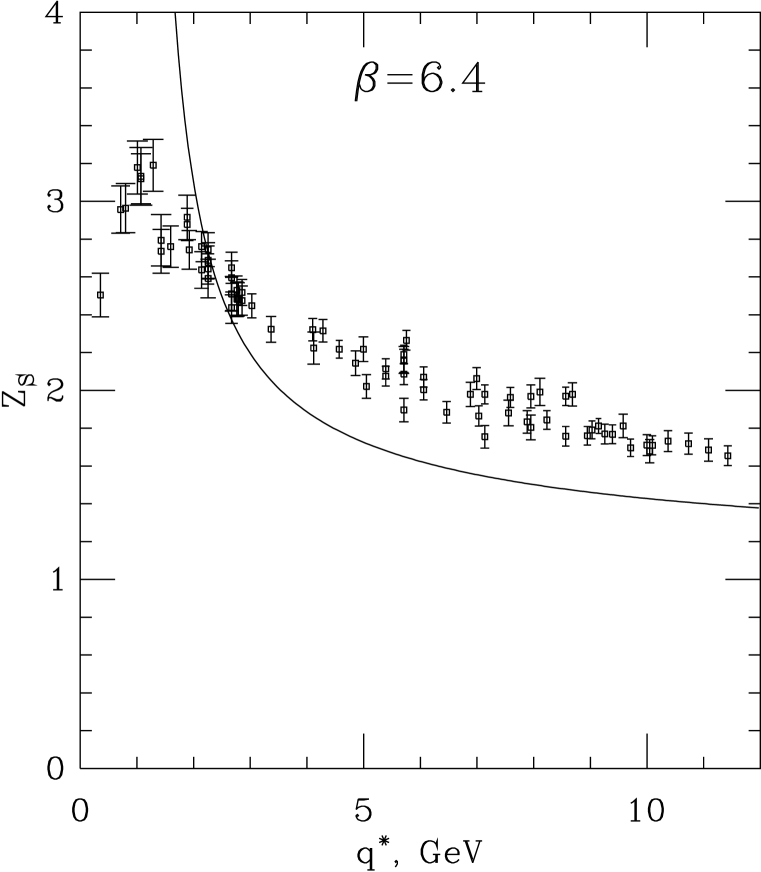
Figure 5.6: $Z_{S}$ at $\beta=6.4$ vs. momentum. Solid curve shows the $Z_{S}$ value calculated in perturbation theory with $g_{\overline{\rm MS}}$ coupling.

We have checked the discrete rotation invariance by comparing results for several momenta related by rotation by $90^{\circ}$ around one or several of the axes. Another interesting check is to compare results obtained with two momenta which have the same $p^{2}$ but different component structure, for example: (1,1,1,1) and (0,0,0,2). This allows one to check for continuous rotation invariance. As expected, this invariance is slightly broken by the lattice cutoff. In the above figures, all kinds of momenta component structures are present. Sometimes, two (or more) momenta have the same $p^{2}$. By looking at the differences in the plotted function between these two momenta it is possible to obtain an indication of the discretization effects. Indeed, these effects grow larger for larger momenta, as expected. In addition, they decrease for any given momentum as $\beta$ grows (i.e., closer to the continuum limit). These effects are discussed more in the next subsection.

5.2.4 Results For Light Quark Masses

Values of light quark masses can be obtained from lattice calculations with staggered fermions as follows. By computing masses of mesons at a variety of bare quark mass values, the values of bare quark masses are obtained by extrapolation to the corresponding physical meson masses. For example, the strange quark mass corresponds to the lattice meson mass being $\sqrt{2}$ times the physical kaon mass (this is because the kaon on the lattice is composed of two equal-mass quarks, while in the real world the kaon is composed of the strange quark and the comparatively massless down-quark; and $m_{K}^{2}\propto(m_{s}+m_{d})$). The bare quark mass in physical units is obtained by dividing the mass in lattice units by $a$:

$$m=\frac{(ma)_{M_{\rm phys}}}{a}\ .$$ (5.19)

This procedure gives the masses of the quarks in lattice regularization scheme. But their values need to be matched to continuum just the same as for the operators, and herein lies a well-known problem, since the perturbative operator matching does not work very well in this case.

To overcome this problem, we use the bilinear renormalization constant $Z_{S}$, computed non-perturbatively as described in the previous subsection. Using

$$Z_{S}=Z_{m}^{-1},$$

we compute the quark masses in $\overline{\rm MS}$ NDR scheme as follows:

$$m^{\rm cont}(\overline{\rm MS}\;{\rm NDR},\mu)=U(\mu,q^{*})Z_{c}(q^{*})Z_{S}^{\rm RI}(q^{*})m^{\rm latt}.$$ (5.20)

Figure 5.7: Strange quark mass at 2 GeV ($\beta=6.4$) vs. the matching momentum scale $p^{2}=q^{*2}$.

Figure 5.8: Strange quark mass at 2 GeV ($\beta=6.4$) vs. the matching momentum scale $p^{2}=q^{*2}$ for the axial and diagonal momentum families.

In Fig. 5.7 I show the results for $m_{s}$ at the scale of 2 GeV in $\overline{\rm MS}$ NDR scheme obtained from a variety of matching momenta at $\beta=6.4$. Ideally, one expects to see a plateau in the middle of the plot, where $p^{2}$ is sufficiently above the hadronization scale, and sufficiently low so that $p^{2}a^{2}\ll 1$. However, the data show (1) sizable dependence on the momentum component structure (a spread along the vertical axis) and (2) a noticeable downward trend. Both are evidently due to the discretization effects, and are expected to be proportional to $p^{2}a^{2}$, which is not unreasonable according to the data. In order to study it more, in Fig. 5.8 I have plotted two families of momenta each having unique component structure but different overall magnitude. These families are: (1) axial, with momenta (0,0,0,1), (0,0,0,2), (0,0,0,4) etc.; and (2) diagonal, with momenta (1,1,1,1), (2,2,2,2) etc. One expects these families to be the opposite extreme cases, with the rest of the momenta being in between them in certain sense. Linear extrapolation to $p^{2}=0$ gives very close results for these two families. Therefore, such an extrapolation is the most natural way to obtain reliable estimates of the quark mass at any given $\beta$, since a large part of the discretization effects is removed.

Figure 5.9: Strange quark mass at 2 GeV, a continuum extrapolation in quenched QCD. Continuum limit results are shown with bursts at $a^{2}=0$.

One can also study the discretization effects by performing continuum extrapolation. This is done in Fig. 5.9 for ensembles with $\beta=6.4$, 6.2 and 6.0. We are using the diagonal family for the extrapolation, since arguably it has minimal discretization corrections. Two sets of data are plotted in Fig. 5.9: one corresponding to using the matching scale $p^{2}=22\ {\rm GeV}^{2}$, and the other one obtained at each $\beta$ by extrapolating to $p^{2}=0$, as discussed above. The results are consistent, which was expected since the discretization errors vanish in continuum limit. This adds to the strength of the hypothesis that the slope and spread in data in Fig. 5.7 is due to discretization effects.

As our best estimate we quote the value of the strange quark mass in quenched QCD:

$$m_{s}(\overline{\rm MS}\;{\rm NDR},2\;{\rm GeV},a=0)=102.9\pm 5.1\;{\rm MeV}.$$ (5.21)

This was obtained by extrapolating to $p^{2}=0$ at each $\beta$. The mass $\overline{m}\equiv(m_{u}+m_{d})/2$ can be obtained by dividing the above value by 26, according to chiral perturbation theory. Our results agree with those of the JLQCD group [19], which were obtained with a slightly different nonperturbative method. These results are also consistent with those obtained with $O(a)$ improved Wilson fermions [20]. To close the discussion of light quark masses, I report the result for dynamical $N_{f}=2$ ensemble at $\beta=5.7$:

$$m_{s}(\overline{\rm MS}\;{\rm NDR},2\;{\rm GeV})=105.1\pm 16.4\;{\rm MeV}.$$ (5.22)

At current level of precision, the dynamical result is consistent with the quenched ones.

5.3 Partially Nonperturbative Matching For Basis Operators.

Ideally, one would like to perform a matching procedure for four-fermion operators, not only for bilinears. It is quite conceivable that such a procedure will be done in the nearest future. As a temporary solution, however, we have adopted a partially nonperturbative operator matching procedure, which makes use of bilinear renormalization coefficients $Z_{P}$ and $Z_{S}$ computed in the previous section. An estimate of the renormalization of four-fermion operators can be obtained as follows.

Figure 5.10: Example of one loop diagrams arising in renormalization of four-fermion operators: in type (a) no propagator crosses the axis, and type (b) includes the rest of the diagrams.

Consider renormalization of the pseudoscalar–pseudoscalar operator in Eq. (5.2). At one-loop level, the diagonal renormalization coefficient $C_{PP}$ (involving diagrams shown in Fig. 5.10) is almost equal to twice the pseudoscalar bilinear correction $C_{P}$. This suggests that, at least at one-loop level, the renormalization of $(PP)_{EU}$ comes mostly from diagrams in which no gluon propagator crosses the vertical axis of the diagram (for example, diagram $(a)$ in Fig. 5.10), and very little from the rest of the diagrams (such as diagram $(b)$ in Fig. 5.10). In other words, the renormalization of $(PP)_{EU}$ would be identical to the renormalization of product of two pseudoscalar bilinears, were it not for the diagrams of type $(b)$, which give a subdominant contribution. Mathematically,

$$(PP)_{EU}^{\mathrm{cont}}=(PP)_{EU}^{\mathrm{latt}}\;Z_{PP}+...\,,$$

with

$$Z_{PP}=Z_{P}^{2}(1+\frac{g^{2}}{16\pi^{2}}\widetilde{C_{PP}}+O(g^{4}))\,,$$ (5.23)

$$Z_{P}=1+\frac{g^{2}}{16\pi^{2}}C_{P}+O(g^{4})\,,$$ (5.24)

and dots indicate mixing with other operators (non-diagonal part). The factor $\widetilde{C_{PP}}\equiv C_{PP}-2C_{P}$ contains diagrams of type $(b)$ in Fig. 5.10 and is quite small.

In order to proceed, it may be reasonable to assume that the same holds at all orders in perturbation theory; namely the diagrams of type $(c)$ in Fig. 5.1 give subdominant contribution compared to type $(a)$ of the same Figure. This assumption should be verified separately by performing non-perturbative renormalization procedure for four-fermion operators. If this ansatz is true, we can substitute the non-perturbative value of $Z_{P}$ into Eq. (5.23) instead of using the perturbative expression from Eq. (5.24). Thus a partially nonperturbative estimate of $(PP)_{U}^{\mathrm{c}ont}$ is obtained. This procedure is quite similar to the tadpole improvement idea: the bulk of diagonal renormalization is calculated non-perturbatively, while the rest is reliably computed in perturbation theory. Analogously we obtain diagonal renormalization of operators $(SS)_{IU}$ and $(PS)_{A2U}$ by using $Z_{SS}=Z_{S}^{2}(1+\frac{g^{2}}{16\pi^{2}}\widetilde{C_{SS}}+O(g^{4}))$ and $Z_{PS}=Z_{S}Z_{P}(1+\frac{g^{2}}{16\pi^{2}}\widetilde{C_{PS}}+O(g^{4}))$. (Note that $Z_{P}\neq Z_{S}$, even though they are equal in perturbation theory.) We match operators at the scale $q^{*}=1/a$ and use the continuum two-loop anomalous dimension to evolve to $\mu=2$ GeV.

Unfortunately, the above procedure does not solve completely the problem of operator renormalization, since it deals only with diagonal renormalization of the zero-distance operators in Eqs. (5.2)—(5.4). Even though these operators are dominant in contributing to $\varepsilon^{\prime}/\varepsilon$, other operators (such as $(SS)_{EU}$ and $(PP)_{EF}$) can be important due to mixing with the dominant ones. The mixing coefficients for these operators are not known even in perturbation theory. For a reasonable estimate we use the coefficients obtained for gauge non-invariant operator mixing [51].

Secondly, since renormalization of operators $(PP)_{EU}$, $(SS)_{IU}$ and $(PS)_{A2U}$ is dramatic, their influence on other operators through non-diagonal mixing is ambiguous at one-loop order, even if the mixing coefficients are known. The ambiguity is due to higher order diagrams (for example, those shown in Fig. 5.1). In order to partially resum them we use operators $(PP)_{EU}$, $(SS)_{IU}$ and $(PS)_{A2U}$ multiplied by factors $Z_{P}^{2}$, $Z_{S}^{2}$ and $Z_{P}Z_{S}$, correspondingly, whenever they appear in non-diagonal mixing with other operators. This is equivalent to evaluating the diagrams of type ($a$) and ($b$) in Fig. 5.1 at all orders, but ignoring the rest of the diagrams (such as diagrams ($c$) and ($d$) in Fig 5.1) at all orders higher than first. A completely analogous procedure was used for mixing of $O_{6}$ with $O_{2}$ through penguins when evaluating $\mbox{Re}A_{0}$. To estimate a possible error in this procedure we compare with a simpler one, whereby bare operators are used in non-diagonal corrections (i.e. we apply strictly one-loop renormalization). The difference in $\varepsilon^{\prime}/\varepsilon$ between these two approaches is of the same order or even less than the error due to uncertainties in determination of $Z_{P}$ and $Z_{S}$ (see Tables 5.3 and 5.4).

Quark	0.01	0.02	0.03
mass
M1 (p.r.)	$-61.2\pm 2.8\pm 10.6$	$-27.4\pm 0.9\pm 8.9$	$-16.8\pm 0.5\pm 8.0$
M1 (1-loop.)	$-52.3\pm 2.2\pm 10$	$-22.0\pm 0.8\pm 8.3$	$-12.2\pm 0.5\pm 6.9$
M2 (p.r.)	$-38.6\pm 2.1\pm 6.0$	$-18.7\pm 0.3\pm 7.0$	$-11.7\pm 0.2\pm 6.0$
M2 (1-loop)	$-45.4\pm 3.5\pm 8.6$	$-18.8\pm 0.4\pm 7.0$	$-10.3\pm 0.3\pm 6.0$
M3 (p.r.)	$-97\pm 14\pm 13$	$-81\pm 4\pm 23$	$-79\pm 2\pm 27$
M3 (1-loop)	$-142\pm 28\pm 29$	$-88\pm 5\pm 35$	$-75\pm 2\pm 39$

Quark	0.04	0.05
mass
M1 (p.r.)	$-8.0\pm 0.9\pm 7.2$	$-4.4\pm 0.9\pm 7.2$
M1 (1-loop)	$-4.2\pm 1.1\pm 6.5$	$-1.2\pm 1.0\pm 6.6$
M2 (p.r.)	$-6.1\pm 0.5\pm 5.3$	$-3.1\pm 0.5\pm 4.9$
M2 (1-loop)	$-3.7\pm 0.8\pm 5.8$	$-0.9\pm 0.8\pm 5.2$
M3 (p.r.)	$-81\pm 5\pm 38$	$-74\pm 4\pm 38$
M3 (1-loop)	$-64\pm 4\pm 52$	$-55\pm 5\pm 51$

Table 5.3: $\varepsilon^{\prime}/\varepsilon$ in units of $10^{-4}$ for $Q_{1}$ ensemble ($\beta=6.0$), computed in three ways mentioned in text. In all cases, partially-nonperturbative matching have been used to obtain the results.

Quark mass	0.005	0.010	0.015
M1 (p.r.)	$-68.1\pm 6.9\pm 36.0$	$-33.6\pm 2.9\pm 23.9$	$-24.9\pm 1.8\pm 22.0$
M1 (1-loop)	$-60.9\pm 6.9\pm 31.2$	$-29.3\pm 2.9\pm 21.0$	$21.4\pm 1.9\pm 19.4$
M2 (p.r.)	$-43.9\pm 9.5\pm 16.5$	$-33.1\pm 3.8\pm 18.3$	$-22.1\pm 1.2\pm 16.4$
M2 (1-loop)	$-53.6\pm 16.9\pm 25.0$	$-37.9\pm 6.0\pm 25.3$	$-23.0\pm 1.5\pm 20.0$
M3 (p.r.)	$-63.3\pm 35.1\pm 15.5$	$-103.9\pm 31.7\pm 45.2$	$-82.4\pm 12.9\pm 51.0$
M3 (1-loop)	$-98.3\pm 72.9\pm 46.2$	$-138.1\pm 53.1\pm 101.5$	$-92.4\pm 16.3\pm 86.3$

Quark mass	0.020	0.030
M1 (p.r.)	$-14.8\pm 1.0\pm 24.8$	$-10.3\pm 0.6\pm 19.6$
M1 (1-loop)	$-11.8\pm 1.1\pm 21.9$	$-7.9\pm 0.7\pm 17.3$
M2 (p.r.)	$-14.2\pm 0.4\pm 20.3$	$-9.5\pm 0.3\pm 16.1$
M2 (1-loop)	$-13.6\pm 0.6\pm 24.3$	$-8.5\pm 0.5\pm 18.0$
M3 (p.r.)	$-74.9\pm 5.7\pm 88.0$	$-80.4\pm 3.9\pm 92.3$
M3 (1-loop)	$-72.6\pm 5.7\pm 142.0$	$-73.5\pm 4.0\pm 131.0$

Table 5.4: $\varepsilon^{\prime}/\varepsilon$ results for $Q_{3}$ ensemble ($\beta=6.2$).

5.4 Estimates Of $\varepsilon^{\prime}/\varepsilon$

Within the procedure outlined in the previous section we have found that $\langle O_{6}\rangle$ has a different sign from the expected one due to a large renormalization factor. This translates into a negative or very slightly positive value of $\varepsilon^{\prime}/\varepsilon$ (Tables 5.3 and 5.4 and Fig. 5.11).

Tables 5.3 and 5.4 contain our results for $\varepsilon^{\prime}/\varepsilon$ obtained in the above-described procedure. In all perturbative corrections we have used one-loop non-diagonal coefficients computed for gauge-noninvariant operators, which are assumed to be of the same order as those for gauge-invariant operators. The first quoted error is statistical (obtained by combining the individual errors in matrix elements by jackknife). The second error is the diagonal operator matching error due to uncertainty in the determination of $Z_{P}$ and $Z_{S}$. In order to estimate the non-diagonal operator matching error we compare two renormalization procedures: using strictly one-loop non-diagonal corrections (denoted “(1-loop)”), and resumming part of higher-order corrections in non-diagonal mixing by using non-perturbative renormalization factors $Z_{P}$ and $Z_{S}$ (as explained in Section 5.3). The latter method is denoted “(p.r.)”.

Finite volume and quenching effects were found small compared to noise. In addition to the quoted errors, there are uncertainties due to an unknown degree of validity of our ansatz in Sec. 5.3, and due to unknown non-diagonal coefficients in the mixing matrix. The former error is uncontrolled at this point, since it is difficult to rigorously check our assumption made in Sec. 5.3. The latter error is likely to be of the same order as the spread in $\varepsilon^{\prime}/\varepsilon$ between two different approaches to higher-order corrections (strictly one-loop and partial resummation), studied in Tables 5.3 and 5.4.

Some other parameters used in obtaining these results are: $\mbox{Im}\lambda_{t}=1.5\cdot 10^{-4}$, $m_{t}=170$ GeV, $m_{b}=4.5$ GeV, $m_{c}=1.3$ GeV, $\Omega_{\eta+\eta^{\prime}}=0.25$, $\alpha^{(n_{f}=0)}_{\overline{\mathrm{M}S}}(2\quad{\mathrm{G}eV})=0.195$ (the latter is based on setting the lattice scale by $\rho$ meson mass). Short distance coefficients were obtained by two-loop running using the anomalous dimension and threshold matrices computed by Buras et al. [58].

Note that there are several choices to make in using our data to estimate $\varepsilon^{\prime}/\varepsilon$. One can use the experimental values of $\mbox{Re}A_{0}$ and $\mbox{Re}A_{2}$ in Eq. (2.17) (M1), or one can use the values obtained on the lattice (M3). One can also adopt an intermediate strategy (M2) of using the experimental amplitude ratio $\omega$ and computed $\mbox{Re}A_{0}$. When the higher-order chiral corrections are taken into account and the continuum limit is taken (so that $\omega=22$), these three methods should converge. The method M2 is preferred, since in this method the overall error due to final state interactions cancels between real and imaginary parts of $A_{0}$ amplitude, while the relative size of $\Pi_{0}$ and $\Pi_{2}$ contributions is given by the physical $\omega$.

Figure 5.11: A rough estimate of $\varepsilon^{\prime}/\varepsilon$ for $Q_{1}$ ($\beta=6.0$) ensemble using the partially-nonperturbative procedure described in text. The Fermilab result’s central value is shown with a horizontal line. The points are displaced horizontally for convenience.

Fig. 5.11 presents the data obtained on ensemble $Q_{1}$, with error bars showing all three errors quoted in Tables 5.3 and 5.4, combined in quadrature.

Figure 5.12: A study of cutoff dependence of $\varepsilon^{\prime}/\varepsilon$ . Plotted are data obtained on $\beta=6.0$ and $\beta=6.2$ ensembles for M2 method. The error bars show only the statistical error in matrix elements and in $Z_{S}$ and $Z_{P}$ constants. Systematic errors are significant but common to both ensembles.

Fig. 5.12 contains comparison of results for $\varepsilon^{\prime}/\varepsilon$ on $\beta=6.0$ and $\beta=6.2$ ensembles. With current errors, the cutoff dependence of $\varepsilon^{\prime}/\varepsilon$ does not appear to be significant. The errors shown are purely statistical.

5.5 Summary

I have shown that perturbative operator matching conventionally employed in lattice calculations breaks down in the case of estimating $\varepsilon^{\prime}/\varepsilon$ . A partially nonperturbative procedure is proposed as a temporary resolution. Light quark masses and (pseudo)scalar bilinear renormalization constants have been computed nonperturbatively.

Our best result (at kaon mass, $\beta=6.0$, M2 method) is

$$\mbox{Re}(\varepsilon^{\prime}/\varepsilon)=(-38.6\pm 9.3)\cdot 10^{-4}\ .$$ (5.25)

The quoted error is a combination of the statistical and several known systematic errors. The reader should keep in mind that additional systematic errors present are very difficult to estimate. These errors are due to higher-order chiral terms (of the order of 40 %) and due to neglecting certain types of higher-order diagrams in partially nonperturbative operator matching.

Taken at face value, our present estimate of $\varepsilon^{\prime}/\varepsilon$ would contradict the present experimental results, which favor a positive value. Therefore, the minimal Standard Model’s description of direct CP violation would be proved to be invalid. At this point, it is too early to draw strong conclusions, since potentially large systematic uncertainties are present in our estimates.

A recent study of $\varepsilon^{\prime}/\varepsilon$ with domain wall fermions by the RIKEN-BNL-Columbia group [18] has also produced negative values for $\varepsilon^{\prime}/\varepsilon$ . While this consistency is encouraging (in particular, it shows that the assumptions made in our operator matching procedure do not change the qualitative picture), the reader should keep in mind that the errors due to using lowest-order chiral perturbation theory are common to both ours and RIKEN-BNL-Columbia calculations.

Chapter 6 Conclusions

In this thesis I report the techniques and results of work directed at calculating hadronic matrix elements of $\Delta S=1$ basis operators in Lattice QCD. Matrix elements of all basis operators have been computed with good statistical precision. Combined with lowest-order chiral perturbation theory, they allow one to make a theoretical prediction for $\Delta I=1/2$ rule and direct CP violation parameter $\varepsilon^{\prime}/\varepsilon$ .

Based on the minimal Standard Model, we predict a substantial enhancement of $\Delta I=1/2$ transitions with respect to $\Delta I=3/2$ ones, consistent with experimental observations, although the exact amount of enhancement is subject to large systematic uncertainties due to higher-order chiral terms. Thus our calculations confirm the currently dominant view that most of the enhancement comes from strong interactions.

A theoretical prediction for $\varepsilon^{\prime}/\varepsilon$ is also made. Evaluated within the minimal Standard Model framework, $\varepsilon^{\prime}/\varepsilon$ is found to have a negative value, in apparent conflict with experiments, although our prediction at present suffers from large systematic error. In the future, it is possible to improve the accuracy of this prediction by performing fully nonperturbative operator matching as well as including higher orders in the chiral expansion. These improvements will come at a relatively easy computational cost, since the main results of our calculation (matrix elements $\langle\pi^{+}|O_{i}|K^{+}\rangle$ and $\langle 0|O_{i}|K^{0}\rangle$ in the lattice regularization scheme, which require most of the computational power) can be used along with above-mentioned improvements without repeating the calculations. If the sign of $\varepsilon^{\prime}/\varepsilon$ stays negative after these improvements, this would be the first failure of the minimal Standard Model to describe the real-world data, and so would have profound consequences in particle physics.

In addition, we have computed light quark masses using nonperturbative renormalization.

Appendix A Explicit expressions for matrix elements in terms of fermion contractions.

Operators in Eqs. (2.2)–2.11) can be decomposed into $I=0$ and $I=2$ parts, which contribute, correspondingly, to $\Delta I=1/2$ and $\Delta I=3/2$ transitions. Here we give the expressions for these parts for completeness, since $\mbox{Re}A_{0}$, $\mbox{Re}A_{2}$ and $\varepsilon^{\prime}/\varepsilon$ are directly expressible in terms of their matrix elements. The $I=0$ parts are given as follows:

$$O_{1}^{(0)} = \frac{2}{3}(\overline{s}\gamma_{\mu}(1-\gamma_{5})d)(\overline{u}\gamma^{\mu}(1-\gamma_{5})u)-\frac{1}{3}(\overline{s}\gamma_{\mu}(1-\gamma_{5})u)(\overline{u}\gamma^{\mu}(1-\gamma_{5})d)$$ (A.1)

$$+ \frac{1}{3}(\overline{s}\gamma_{\mu}(1-\gamma_{5})d)(\overline{d}\gamma^{\mu}(1-\gamma_{5})d)$$

$$O_{2}^{(0)} = \frac{2}{3}(\overline{s}\gamma_{\mu}(1-\gamma_{5})u)(\overline{u}\gamma^{\mu}(1-\gamma_{5})d)-\frac{1}{3}(\overline{s}\gamma_{\mu}(1-\gamma_{5})d)(\overline{u}\gamma^{\mu}(1-\gamma_{5})u)$$ (A.2)

$$+ \frac{1}{3}(\overline{s}\gamma_{\mu}(1-\gamma_{5})d)(\overline{d}\gamma^{\mu}(1-\gamma_{5})d)$$

$$O_{3}^{(0)} = (\overline{s}\gamma_{\mu}(1-\gamma_{5})d)\sum_{q=u,d,s}(\overline{q}\gamma^{\mu}(1-\gamma_{5})q)$$ (A.3)

$$O_{4}^{(0)} = (\overline{s}_{\alpha}\gamma_{\mu}(1-\gamma_{5})d_{\beta})\sum_{q=u,d,s}(\overline{q}_{\beta}\gamma^{\mu}(1-\gamma_{5})q_{\alpha})$$ (A.4)

$$O_{5}^{(0)} = (\overline{s}\gamma_{\mu}(1-\gamma_{5})d)\sum_{q=u,d,s}(\overline{q}\gamma^{\mu}(1+\gamma_{5})q)$$ (A.5)

$$O_{6}^{(0)} = (\overline{s}_{\alpha}\gamma_{\mu}(1-\gamma_{5})d_{\beta})\sum_{q=u,d,s}(\overline{q}_{\beta}\gamma^{\mu}(1+\gamma_{5})q_{\alpha})$$ (A.6)

$$O_{7}^{(0)} = \frac{1}{2}[(\overline{s}\gamma_{\mu}(1-\gamma_{5})d)(\overline{u}\gamma^{\mu}(1+\gamma_{5})u)-(\overline{s}\gamma_{\mu}(1-\gamma_{5})u)(\overline{u}\gamma^{\mu}(1+\gamma_{5})d)$$ (A.7)

$$- (\overline{s}\gamma_{\mu}(1-\gamma_{5})d)(\overline{s}\gamma^{\mu}(1+\gamma_{5})s)]$$

$$O_{8}^{(0)} = \frac{1}{2}[(\overline{s}_{\alpha}\gamma_{\mu}(1-\gamma_{5})d_{\beta})(\overline{u}_{\beta}\gamma^{\mu}(1+\gamma_{5})u_{\alpha})-(\overline{s}_{\alpha}\gamma_{\mu}(1-\gamma_{5})u_{\beta})(\overline{u}_{\beta}\gamma^{\mu}(1+\gamma_{5})d_{\alpha})$$ (A.8)

$$- (\overline{s}_{\alpha}\gamma_{\mu}(1-\gamma_{5})d_{\beta})(\overline{s}_{\beta}\gamma^{\mu}(1+\gamma_{5})s_{\alpha})]$$

$$O_{9}^{(0)} = \frac{1}{2}[(\overline{s}\gamma_{\mu}(1-\gamma_{5})d)(\overline{u}\gamma^{\mu}(1-\gamma_{5})u)-(\overline{s}\gamma_{\mu}(1-\gamma_{5})u)(\overline{u}\gamma^{\mu}(1-\gamma_{5})d)$$ (A.9)

$$- (\overline{s}\gamma_{\mu}(1-\gamma_{5})d)(\overline{s}\gamma^{\mu}(1-\gamma_{5})s)]$$

$$O_{10}^{(0)} = \frac{1}{2}[(\overline{s}\gamma_{\mu}(1-\gamma_{5})u)(\overline{u}\gamma^{\mu}(1-\gamma_{5})d)-(\overline{s}\gamma_{\mu}(1-\gamma_{5})d)(\overline{u}\gamma^{\mu}(1-\gamma_{5})u)$$ (A.10)

$$- (\overline{s}\gamma_{\mu}(1-\gamma_{5})d)(\overline{s}\gamma^{\mu}(1-\gamma_{5})s)]$$

Expressions for $I=2$ parts are as follows:

$$O_{1}^{(2)} = O_{2}^{(2)}=\frac{2}{3}O_{9}^{(2)}=\frac{2}{3}O_{10}^{(2)}=\frac{1}{3}[(\overline{s}\gamma_{\mu}(1-\gamma_{5})u)(\overline{u}\gamma^{\mu}(1-\gamma_{5})d)$$ (A.11)

$$+(\overline{s}\gamma_{\mu}(1-\gamma_{5})d)(\overline{u}\gamma^{\mu}(1-\gamma_{5})u)-(\overline{s}\gamma_{\mu}(1-\gamma_{5})d)(\overline{d}\gamma^{\mu}(1-\gamma_{5})d)]$$

$$O_{7}^{(2)} = \frac{1}{2}[(\overline{s}\gamma_{\mu}(1-\gamma_{5})u)(\overline{u}\gamma^{\mu}(1+\gamma_{5})d)+(\overline{s}\gamma_{\mu}(1-\gamma_{5})d)(\overline{u}\gamma^{\mu}(1+\gamma_{5})u)$$ (A.12)

$$-(\overline{s}\gamma_{\mu}(1-\gamma_{5})d)(\overline{d}\gamma^{\mu}(1+\gamma_{5})d)]$$

$$O_{8}^{(2)} = \frac{1}{2}[(\overline{s}_{\alpha}\gamma_{\mu}(1-\gamma_{5})u_{\beta})(\overline{u}_{\beta}\gamma^{\mu}(1+\gamma_{5})d_{\alpha})+(\overline{s}_{\alpha}\gamma_{\mu}(1-\gamma_{5})d_{\beta})(\overline{u}_{\beta}\gamma^{\mu}(1+\gamma_{5})u_{\alpha})$$ (A.13)

$$-(\overline{s}_{\alpha}\gamma_{\mu}(1-\gamma_{5})d_{\beta})(\overline{d}_{\beta}\gamma^{\mu}(1+\gamma_{5})d_{\alpha})]$$

$$O_{3}^{(2)} = O_{4}^{(2)}=O_{5}^{(2)}=O_{6}^{(2)}=0$$ (A.14)

(Whenever the color indices are not shown, they are contracted within each bilinear, i.e. there are two color traces.)

As mentioned in Sec. 3.2.3, in order to compute matrix elements of $I=0$ operators one needs to evaluate three types of diagrams: “eight” (Fig. 3.2a), “eye” (Fig. 3.2b) and “annihilation” (Fig. 3.2c). In the previous Appendix section we have given detailed expressions for computation of these contractions, given the spin-flavor structure. Here we assign this structure to all contractions required for each operator, i.e. we express each matrix element in terms of contractions which were “built” in the previous section.

Let us introduce some notation. The matrix element of the above operators have three components:

$$\langle\pi^{+}\pi^{-}|O_{i}|K^{0}\rangle=(E_{i}+I_{i}-S\,(\,2\,m\alpha_{i})\,)\,\frac{m_{K}^{2}-m_{\pi}^{2}}{(p_{\pi}\cdot p_{K})f},$$ (A.15)

where $m$ is the common quark mass for $s$, $d$ and $u$, and

$$\alpha_{i}=\frac{A_{i}}{P}.$$ (A.16)

Here $E_{i}$ and $I_{i}$ stand for “eight and “eye” contractions of the $\langle\pi^{+}|O_{i}|K^{+}\rangle$ matrix element, $A_{i}\sim\langle 0|O_{i}|K^{0}\rangle\,/\,(m_{d}-m_{s})$ is the “annihilation” diagram, $S=\langle\pi^{+}|\overline{s}d|K^{+}\rangle$ is the “subtraction” diagram, and $P=\langle 0|\overline{s}\gamma_{5}d|K^{0}\rangle$ is the two-point function. We compute $\alpha_{i}$ by averaging the ratio in the right-hand side of Eq. (A.16) over a suitable time range.

Detailed expressions for $E_{i}$, $I_{i}$ and $A_{i}$ are given below in terms of the basic contractions on the lattice. We label basic contractions by two letters, each representing a bilinear. For example, $PP$ stands for contraction of the operator with spin structure $(\gamma_{5})(\gamma_{5})$, $SS$ is for $({\displaystyle\mathbf{1}})({\displaystyle\mathbf{1}})$, $VV$ stands for $(\gamma_{\mu})(\gamma^{\mu})$, and $AA$ is for $(\gamma_{\mu}\gamma_{5})(\gamma^{\mu}\gamma_{5})$. The staggered flavor is determined by the type of contraction, as explained in the previous Appendix section. Basic contractions are also labeled by their subscript. The first letter indicates whether it is an “eight”, “eye” or “annihilation” contraction, and the second is “U” for two, or “F” for one color trace. For example: $PP_{EU}$ stands for the “eight” contraction of the operator with spin-flavor structure $(\gamma_{5}\otimes\xi_{5})(\gamma_{5}\otimes\xi_{5})$ with two color traces; $VA_{A1F}$ stands for the “annihilation” contraction of the first type, in which the derivative is taken with respect to quark mass on the external leg (see the previous Appendix section), the spin-flavor structure is $(\gamma_{\mu}\otimes\xi_{5})(\gamma^{\mu}\gamma_{5}\otimes{\displaystyle\mathbf{1}})$, and one color trace is taken. What follows are the full expressions.

“Eight” parts:

$$E_{1}^{(0)} = \frac{2}{3}(VV_{EF}+AA_{EF})-\frac{1}{3}(VV_{EU}+AA_{EU})$$ (A.17)

$$E_{2}^{(0)} = \frac{2}{3}(VV_{EU}+AA_{EU})-\frac{1}{3}(VV_{EF}+AA_{EF})$$ (A.18)

$$E_{3}^{(0)} = VV_{EF}+AA_{EF}$$ (A.19)

$$E_{4}^{(0)} = VV_{EU}+AA_{EU}$$ (A.20)

$$E_{5}^{(0)} = 2(PP_{EF}-SS_{EF})$$ (A.21)

$$E_{6}^{(0)} = 2(PP_{EU}-SS_{EU})$$ (A.22)

$$E_{7}^{(0)} = SS_{EF}-PP_{EF}+\frac{1}{2}(VV_{EU}-AA_{EU})$$ (A.23)

$$E_{8}^{(0)} = SS_{EU}-PP_{EU}+\frac{1}{2}(VV_{EF}-AA_{EF})$$ (A.24)

$$E_{9}^{(0)} = -E_{10}^{(0)}=\frac{1}{2}(VV_{EF}+AA_{EF}-VV_{EU}-AA_{EU})$$ (A.25)

$$E_{1}^{(2)} = E_{2}^{(2)}=\frac{2}{3}E_{9}^{(2)}=\frac{2}{3}E_{10}^{(2)}=\frac{1}{3}(VV_{EU}+AA_{EU}+VV_{EF}+AA_{EF})$$ (A.26)

$$E_{3}^{(2)} = E_{4}^{(2)}=E_{5}^{(2)}=E_{6}^{(2)}=0$$ (A.27)

$$E_{7}^{(2)} = \frac{1}{2}(AA_{EU}-VV_{EU})+SS_{EF}-PP_{EF}$$ (A.28)

$$E_{8}^{(2)} = \frac{1}{2}(AA_{EF}-VV_{EF})+SS_{EU}-PP_{EU}$$ (A.29)

“Eye” parts:

$$I_{1}^{(0)} = VV_{IU}+AA_{IU}$$ (A.30)

$$I_{2}^{(0)} = VV_{IF}+AA_{IF}$$ (A.31)

$$I_{3}^{(0)} = 3(VV_{IU}+AA_{IU})+2(VV_{IF}+AA_{IF})$$ (A.32)

$$I_{4}^{(0)} = 3(VV_{IF}+AA_{IF})+2(VV_{IU}+AA_{IU})$$ (A.33)

$$I_{5}^{(0)} = 3(VV_{IU}-AA_{IU})+4(PP_{IF}-SS_{IF})$$ (A.34)

$$I_{6}^{(0)} = 3(VV_{IF}-AA_{IF})+4(PP_{IU}-SS_{IU})$$ (A.35)

$$I_{7}^{(0)} = 2(PP_{IF}-SS_{IF})$$ (A.36)

$$I_{8}^{(0)} = 2(PP_{IU}-SS_{IU})$$ (A.37)

$$I_{9}^{(0)} = VV_{IF}+AA_{IF}$$ (A.38)

$$I_{10}^{(0)} = VV_{IU}+AA_{IU}$$ (A.39)

“Annihilation” parts are obtained by inserting the derivative with respect to $(m_{d}-m_{s})$ into every propagator involving the strange quark:

$$A_{1}^{(0)} = -(VA_{A1U}+AV_{A1U})$$ (A.40)

$$A_{2}^{(0)} = -(VA_{A1F}+AV_{A1F})$$ (A.41)

$$A_{3}^{(0)} = -3(VA_{A1U}+AV_{A1U})-(VA_{A2U}+AV_{A2U})$$ (A.42)

$$-2(VA_{A1F}+AV_{A1F})-(VA_{A2F}+AV_{A2F})$$

$$A_{4}^{(0)} = -3(VA_{A1F}+AV_{A1F})-(VA_{A2F}+AV_{A2F})$$ (A.43)

$$-2(VA_{A1U}+AV_{A1U})-(VA_{A2U}+AV_{A2U})$$

$$A_{5}^{(0)} = 3(VA_{A1U}-AV_{A1U})+(VA_{A2U}-AV_{A2U})+2(PS_{A2F}-SP_{A2F})$$ (A.44)

$$A_{6}^{(0)} = 3(VA_{A1F}-AV_{A1F})+(VA_{A2F}-AV_{A2F})+2(PS_{A2U}-SP_{A2U})$$ (A.45)

$$A_{7}^{(0)} = \frac{1}{2}(VA_{A2U}-AV_{A2U})+(PS_{A2F}-SP_{A2F})$$ (A.46)

$$A_{8}^{(0)} = \frac{1}{2}(VA_{A2F}-AV_{A2F})+(PS_{A2U}-SP_{A2U})$$ (A.47)

$$A_{9}^{(0)} = VA_{A1F}+AV_{A1F}+\frac{1}{2}(VA_{A2U}+AV_{A2U}+VA_{A2F}+AV_{A2F})$$ (A.48)

$$A_{10}^{(0)} = VA_{A1U}+AV_{A1U}+\frac{1}{2}(VA_{A2F}+AV_{A2F}+VA_{A2U}+AV_{A2U})$$ (A.49)

Of course, “eye” and “annihilation” contractions are not present in $I=2$ operators.

References

- [1] P. Shawhan, presentation of KTeV results at Fermilab, February 24, 1999; Fermilab press release, March 1, 1999.
- [2] Talk by P. Debu on behalf of NA48 experiment at CERN, http://www.cern.ch/NA48/FirstResult/slides.html .
- [3] G. D. Barr et al. (NA31 CERN), Phys. Lett. B 317, 233 (1990).
- [4] A. Buras et al., Phys. Lett. B 389, 749 (1996); M. Ciuchini, Nucl. Phys. Proc. Suppl. 59, 149 (1997); M. Ciuchini et al., Z. Phys. C 68, 239 (1995), hep-ph/9501265; S. Bertolini et al., hep-ph/9802405.
- [5] S. Bosch et al., hep-ph/9904408.
- [6] A. Buras et al., Nucl. Phys. B 408, 209-285 (1993), hep-ph/9303284; A. Buras, hep-ph/9806471, to appear in “Probing the Standard Model of Particle Interactions”, F.David and R. Gupta, eds., 1998, Elsevier Science B.V.
- [7] R. Gupta, hep-ph/9801412.
- [8] T. Hambye and P.H. Soldan, hep-ph/9908232; T. Hambye et al., hep-ph/9906434.
- [9] Bertolini et al., Nucl. Phys. B 514, 63 (1998); ibid 93.
- [10] G. Kilcup, Nucl. Phys. B (Proc. Suppl.) 20, 417 (1991); S. Sharpe, Nucl. Phys. B (Proc. Suppl.) 20, 429 (1991); S. Sharpe et al., Phys. Lett. 192B, 149 (1987).
- [11] C. Bernard, T. Draper, G. Hockney, A. Soni, Nucl. Phys. B (Proc. Suppl.) 4, 483 (1988)
- [12] C. Bernard, A. Soni, Nucl. Phys. B (Proc. Suppl.) 17, 495 (1990).
- [13] M.B. Gavela et al., Nucl. Phys. (Proc. Suppl. 7A), 228 (1989); Phys. Lett. 211 B, 139 (1988); E. Franco et al., Nucl. Phys. B (Proc. Suppl.) 4, 466 (1988).
- [14] G. Martinelli et al., Nucl. Phys. B (Proc.Suppl.) 17, 523 (1990);
- [15] C. Bernard, A. Soni, Nucl. Phys. B (Proc. Suppl.) 9, 155 (1989).
- [16] C. Bernard, “Weak Matrix elements on and off the lattice”, in “From Actions To Answers”, proceedings of TASI 1989, eds. T. DeGrand and D. Toussaint, World Scientific, p.233.
- [17] S. Aoki et al. (JLQCD collaboration), Phys. Rev. D 58, 054503 (1998), hep-lat/9711046.
- [18] T. Blum et al. (RIKEN-BNL-Columbia collaboration), hep-lat/9908025.
- [19] S. Aoki et al. (JLQCD collaboration), Phys. Rev. Lett. 82, 4392 (1999).
- [20] M. Gockeler et al., hep-lat/9908028; J. Garden et al., hep-lat/9906013; D. Becirevic et al., Phys. Lett. B 444, 401 (1998); D. Becirevic et al., hep-lat/9909082.
- [21] J. Bijnens et al., Phys. Lett. B 348, 226 (1995); K.G. Chetyrkin et al., Phys. Lett. B 404, 337 (1997).
- [22] T. Bhattacharya et al., Phys. Rev. D 57, 5455 (1998); K. Maltman et al. Nucl.Phys. A 631, 497c-501c (1998).
- [23] H. Georgi, “Weak interactions and modern particle theory”,Benjamin/Cummings, Menlo Park, 1984.
- [24] J. Donoghue et al., “Dynamics of the Standard Model”, Cambridge, 1992.
- [25] S. Sharpe, Boulder TASI 1994: 0377-0444, hep-lat/9412243.
- [26] I. Montvay, G. Munster, “Quantum Fields on a Lattice”, Cambridge, 1994.
- [27] R. Guptra, hep-lat/9807028.
- [28] J. Kogut, in “Lattice Gauge Theory Using Parallel Processors”, eds. X. Li, Z. Qiu, H. Ren, Gordon and Breach Science Publishers, 1987, p.1.
- [29] M. Creutz, “Quarks, Gluons and Lattices”, Cambridge, 1983.
- [30] K. Wilson, Phys. Rev. d 10, 2445 (1974); “Quantum Chromodynamics on a lattice”, in “New developments in Quantum Field Theory and Statistical Mechanics”, Cargese, 1976, ed. M. Levy and P.K. Mitter (Plenum Press, New York).
- [31] L.H. Karsten, J. Smit, Nucl. Phys. B 183, 103 (1981).
- [32] H.B. Nielsen, M. Ninomiya, Nucl. Phys. B 185, 20 (1981);erratum: B 195, 541; Nucl. Phys. B 193, 173 (1981)
- [33] K. Wilson, in “New Phenomena in Subnuclear Physics”, ed. A. Zichichi (Plenum Press, New York, 1975), Part A, p.69.
- [34] J. Kogut, L. Susskind, Phys. Rev. D 11, 395 (1974); L. Susskind, Phys. Rev. D 16, 3031 (1977).
- [35] H. Kluberg-Stern et al., Nucl. Phys. B 220, 447 (1983).
- [36] G. Kilcup, S. Sharpe, Nucl. Phys. B 283, 493 (1987).
- [37] S. Sharpe et al., Nucl. Phys. B 286, 253-292 (1987).
- [38] L. Maiani, M. Testa, Phys. Lett. B 245, 585 (1990).
- [39] C. Bernard, T. Draper, A. Soni, H.D. Politzer and M. B. Wise, Phys. Rev. D 32, 2343 (1985).
- [40] M. Golterman, K.C. Leung, Phys. Rev. D 56, 2950 (1997), hep-lat/9702015; M Golterman, E. Pallante, hep-lat/9909069.
- [41] G.P. Lepage, P.B. MacKenzie, Phys. Rev. D 48, 2250 (1993).
- [42] L. Venkataraman, “Lattice Studies of the Meson”, Ph. D. Thesis, The Ohio State University, 1997.
- [43] F. R. Brown et al., Phys. Rev. D 67, 1062 (1991).
- [44] G. Kilcup, D. Pekurovsky, Nucl. Phys. B (Proc. Suppl.) 53, 345 (1997), hep-lat/9609006.
- [45] S. Gottlieb, Nucl. Phys. B (Proc Suppl.) 53, 155 (1997).
- [46] D. Chen, R Mawhinney, Nucl. Phys. B (Proc. Suppl.) 53, 216 (1997).
- [47] J.F.Donoghue, E. Golowich, B.R. Holstein, Phys. Lett. B 119, 412 (1982).
- [48] S. Sharpe, Phys. Rev. D 46, 3146 (1992).
- [49] S. Sharpe, Nucl. Phys. B (Proc.Suppl.) 34, 403 (1994), hep-lat/9312009.
- [50] N. Ishizuka, Y. Shizawa, Phys. Rev. D 49, 3519 (1994), hep-lat/9308008.
- [51] S. Sharpe, A. Patel, hep-lat/9310004.
- [52] R. Gupta, T. Bhattacharya, S. Sharpe, Phys. Rev. D 55, 4036 (1997).
- [53] A.Donini et al., Eur. Phys. J. C 10, 121 (1999); V. Gimenez et al., Nucl. Phys. B 531,429 (1998).
- [54] G. Martinelli, C. Pittori, C.T. Sachrajda, M. Testa, A. Vladikas, Nucl. Phys. B 445, 81 (1995), hep-lat/9411010.
- [55] E.Franco, V. Lubicz, Nucl. Phys. B 531,641 (1998).
- [56] D. Daniel, S. Sheard, Nucl. Phys. B 302, 471 (1988).
- [57] J-R. Cudell et al., hep-lat/9810058.
- [58] A. Buras et al., Nucl. Phys. B 400, 37 (1993), hep-ph/9211304.