Spectral Functions of Hadrons in Lattice QCD

Abstract

Using the maximum entropy method, spectral functions of the pseudo-scalar and vector mesons are extracted from lattice Monte Carlo data of the imaginary time Green’s functions. The resonance and continuum structures as well as the ground state peaks are successfully obtained. Error analysis of the resultant spectral functions is also given on the basis of the Bayes probability theory.

1 Introduction

The spectral functions (SPFs) of hadrons play a special role in physical observables in QCD (See the examples in [1, 2]). However, the lattice QCD simulations so far have difficulties in accessing the dynamical quantities in the Minkowski space, because measurements on the lattice can only be carried out for discrete points in imaginary time. The analytic continuation from the imaginary time to the real time using the noisy lattice data is highly non-trivial and is even classified as an ill-posed problem.

Recently we made a first serious attempt to extract SPFs of hadrons from lattice QCD data without making a priori assumptions on the spectral shape [3]. We use the maximum entropy method (MEM), which has been successfully applied for similar problems in quantum Monte Carlo simulations in condensed matter physics, image reconstruction in crystallography and astrophysics, and so forth [4, 5]. In this report, we present the results for the pseudo-scalar (PS) and vector (V) channels at $T=0$ using the continuum kernel and the lattice kernel of the integral transform. The latter analysis has not been reported in [3].

2 Basic idea of MEM

The Euclidean correlation function $D(\tau)$ of an operator ${\cal O}(\tau,\vec{x})$ and its spectral decomposition at zero three-momentum read

$$D(\tau) = \int\langle{\cal O}^{\dagger}(\tau,\vec{x}){\cal O}(0,\vec{0})\rangle d^{3}x$$

$$= \int_{0}^{\infty}\!\!K(\tau,\omega)A(\omega)d\omega,$$

where $\tau>0$, $\omega$ is a real frequency, and $A(\omega)$ is SPF (or sometimes called the image), which is positive semi-definite. The kernel $K(\tau,\omega)$ is proportional to the Fourier transform of a free boson propagator with mass $\omega$: At $T=0$ in the continuum limit, $K=K_{cont}(\tau,\omega)=\exp(-\tau\omega)$.

Monte Carlo simulation provides $D(\tau_{i})$ on the discrete set of temporal points $0\leq\tau_{i}/a\leq N_{\tau}$. From this data with statistical noise, we need to reconstruct the spectral function $A(\omega)$ with continuous variable $\omega$. This is a typical ill-posed problem, where the number of data is much smaller than the number of degrees of freedom to be reconstructed. This makes the standard likelihood analysis and its variants inapplicable [6] unless strong assumptions on the spectral shape are made. MEM is a method to circumvent this difficulty through Bayesian statistical inference of the most probable image together with its reliability [4].

MEM is based on the Bayes’ theorem in probability theory: $P[X|Y]=P[Y|X]P[X]/P[Y]$, where $P[X|Y]$ is the conditional probability of $X$ given $Y$. The most probable image $A(\omega)$ for given lattice data $D$ is obtained by maximizing the conditional probability $P[A|DH]$, where $H$ summarizes all the definitions and prior knowledge such as $A(\omega)\geq 0$. By the Bayes’ theorem,

$$P[A|DH]\propto P[D|AH]P[A|H],$$ (2)

where $P[D|AH]$ ($P[A|H]$) is called the likelihood function (the prior probability).

For the likelihood function, the standard $\chi^{2}$ is adopted, namely $P[D|AH]=Z_{L}^{-1}\exp(-L)$ with

$$\mbox{}L={1\over 2}\sum_{i,j}(D(\tau_{i})-D^{A}(\tau_{i}))$$ (3)

$$\mbox{\hskip 71.13188pt}\times\,C^{-1}_{ij}(D(\tau_{j})-D^{A}(\tau_{j})).$$

$Z_{L}$ is a normalization factor given by $Z_{L}=(2\pi)^{N/2}\sqrt{\det C}$ with $N={\tau}_{max}/a-{\tau}_{min}/a+1$. $D(\tau_{i})$ is the lattice data averaged over gauge configurations and $D^{A}(\tau_{i})$ is the correlation function defined by the right hand side of (2). $C$ is an $N\times N$ covariance matrix of the data with $N$ being the number of temporal points to be used in the MEM analysis. The lattice data have generally strong correlations among different $\tau$’s, and it is essential to take into account the off-diagonal components of $C$.

Axiomatic construction as well as intuitive ”monkey argument” [7] show that, for positive distributions such as SPF, the prior probability can be written with parameters $\alpha$ and $m$ as $P[A|H\alpha m]=Z_{S}^{-1}\exp(\alpha S)$. Here $S$ is the Shannon-Jaynes entropy,

$$\mbox{}S=$$ (4)

$$\mbox{}\ \ \int_{0}^{\infty}\left[A(\omega)-m(\omega)-A(\omega)\log\left(\frac{A(\omega)}{m(\omega)}\right)\right]d\omega.$$

$Z_{S}$ is a normalization factor: $Z_{S}\equiv\int e^{\alpha S}{\cal D}A$. $\alpha$ is a real and positive parameter and $m(\omega)$ is a real function called the default model.

In the state-of-art MEM [4], the output image $A_{out}$ is given by a weighted average over $A$ and $\alpha$:

$$\mbox{}A_{out}(\omega)$$

$$=\int A(\omega)\ P[A|DH\alpha m]P[\alpha|DHm]\ {\cal D}A\ d\alpha$$

$$\simeq\int A_{\alpha}(\omega)\ P[\alpha|DHm]\ d\alpha.$$ (5)

Here $A_{\alpha}(\omega)$ is obtained by maximizing the ”free-energy”

$$Q\equiv\alpha S-L,$$ (6)

for a given $\alpha$. Here we assumed that $P[A|DH\alpha m]$ is sharply peaked around $A_{\alpha}(\omega)$. $\alpha$ dictates the relative weight of the entropy $S$ (which tends to fit $A$ to the default model $m$) and the likelihood function $L$ (which tends to fit $A$ to the lattice data). Note, however, that $\alpha$ appears only in the intermediate step and is integrated out in the final result. Our lattice data show that the weight factor $P[\alpha|DHm]$, which is calculable using $Q$ [4], is highly peaked around its maximum $\alpha=\hat{\alpha}$. We have also studied the stability of the $A_{out}(\omega)$ against a reasonable variation of $m(\omega)$.

The non-trivial part of the MEM analysis is to find a global maximum of $Q$ in the functional space of $A(\omega)$, which has typically 750 degrees of freedom in our case. We have utilized the singular value decomposition (SVD) of the kernel to define the search direction in this functional space. The method works successfully to find the global maximum within reasonable iteration steps.

3 MEM with mock data

To check our MEM code and to see the dependence of the MEM image on the quality of the data, we made the following test using mock data. (i) We start with an input image $A_{in}(\omega)\equiv\omega^{2}\rho_{in}(\omega)$ in the $\rho$-meson channel which simulates the experimental $e^{+}e^{-}$ cross section. Then we calculate $D_{in}(\tau)$ from $A_{in}(\omega)$ using eq.(2). (ii) By taking $D_{in}(\tau_{i})$ at $N$ discrete points and adding a Gaussian noise, we create a mock data $D_{mock}(\tau_{i})$. The variance of the noise $\sigma(\tau_{i})$ is given by $\sigma(\tau_{i})=b\times D_{in}(\tau_{i})\times\tau_{i}/a$ with a parameter $b$, which controls the noise level [8]. (iii) We construct the output image $A_{out}(\omega)\equiv\omega^{2}\rho_{out}(\omega)$ using MEM with $D_{mock}(\tau_{min}\leq\tau_{i}\leq\tau_{max})$ and compare the result with $A_{in}(\omega)$. In this test, we have assumed that $C$ is diagonal for simplicity.

In Fig.1, we show $\rho_{in}(\omega)$, and $\rho_{out}(\omega)$ for two sets of parameters, (I) and (II). As for $m$, we choose a form $m(\omega)=m_{0}\omega^{2}$ with $m_{0}=0.027$, which is motivated by the asymptotic behavior of $A$ in perturbative QCD, $A(\omega\gg 1{\rm GeV})=(1/4\pi^{2})(1+\alpha_{s}/\pi)\omega^{2}$. The final result is, however, insensitive to the variation of $m_{0}$ even by factor 5 or 1/5. The calculation of $A_{out}(\omega)$ has been done by discretizing the $\omega$-space with an equal separation of 10 MeV between adjacent points. This number is chosen for the reason we shall discuss below. The comparison of the dashed line (set (I)) and the dash-dotted line (set (II)) shows that increasing $\tau_{max}$ and reducing the noise level $b$ lead to better SPFs closer to the input SPF.

We have also checked that MEM can nicely reproduce other forms of the mock SPFs. In particular, MEM works very well to reproduce not only the broad structure but also the sharp peaks close to the delta-function as far as the noise level is sufficiently small.

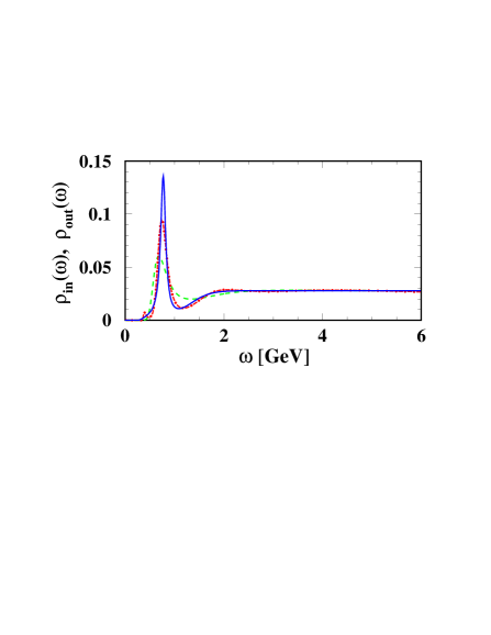
Figure 1: The solid line is $\rho_{in}(\omega)$. The dashed line and dash-dotted line are $\rho_{out}(\omega)$ obtained with parameter set (I) $a=0.0847$ fm, $1\leq\tau/a\leq 12$, $b=0.001$ and set (II) $a=0.0847$ fm, $1\leq\tau/a\leq 36$, $b=0.0001$, respectively.

4 MEM with lattice data

To apply MEM to actual lattice data, quenched lattice QCD simulations have been done with the plaquette gluon action and the Wilson quark action by the open MILC code with minor modifications [9]. The lattice size is $20^{3}\times 24$ with $\beta=6.0$, which corresponds to $a=0.0847$ fm ($a^{-1}=2.33$ GeV), $\kappa_{c}=0.1571$ [10], and the spatial size of the lattice $L_{s}a=1.69$ fm. Gauge configurations are generated by the heat-bath and over-relaxation algorithms with a ratio $1:4$. Each configuration is separated by 1000 sweeps. Hopping parameters are chosen to be $\kappa=$ 0.153, 0.1545, and 0.1557 with $N_{conf}=161$ for each $\kappa$. For the quark propagator, the Dirichlet (periodic) boundary condition is employed for the temporal (spatial) direction. We have also done the simulation with periodic boundary condition in the temporal direction and obtained qualitatively the same results. To calculate the two-point correlation functions, we adopt a point-source at $\vec{x}=0$ and a point-sink averaged over the spatial lattice-points.

We use data at $1\leq\tau_{i}/a\leq 12(24)$ for the Dirichlet (periodic) boundary condition in the temporal direction. To avoid the known pathological behavior of the eigenvalues of $C$ [4], we take $N_{conf}\gg N$.

We define SPFs for the PS and V channels as

$$A(\omega)=\omega^{2}\rho_{{}_{PS},_{V}}(\omega),$$ (7)

so that $\rho_{{}_{PS,V}}(\omega\rightarrow{\rm large})$ approaches a finite constant as predicted by perturbative QCD. For the MEM analysis, we need to discretize the $\omega$-integration in (2). Since $\Delta\omega$ (the mesh size) $\ll 1/\tau_{max}$ should be satisfied to suppress the discretization error, we take $\Delta\omega$ = 10 MeV. $\omega_{max}$ (the upper limit for the $\omega$ integration) should be comparable to the maximum available momentum on the lattice: $\omega_{max}\sim\pi/a\sim 7.3$ GeV. We have checked that larger values of $\omega_{max}$ do not change the result of $A(\omega)$ substantially, while smaller values of $\omega_{max}$ distort the high energy end of the spectrum. The dimension of the image to be reconstructed is $N_{\omega}\equiv\omega_{max}/\Delta\omega\sim 750$, which is in fact much larger than the maximum number of Monte Carlo data $N=25$.

In Fig.2 (a) and (b), we show the reconstructed images for each $\kappa$ in the case of the Dirichlet boundary condition. Here we use the continuum kernel $K_{cont}=\exp(-\tau\omega)$ in the Laplace transform. In these figures, we have used $m=m_{0}\omega^{2}$ with $m_{0}=2.0(0.86)$ for PS (V) channel motivated by the perturbative estimate of $m_{0}$ (see eq.(4) and the text below). We have checked that the result is not sensitive, within the statistical significance of the image, to the variation of $m_{0}$ by factor 5 or 1/5. The obtained images have a common structure: the low-energy peaks corresponding to $\pi$ and $\rho$, and the broad structure in the high-energy region. From the position of the pion peaks in Fig.2(a), we extract $\kappa_{c}=0.1570(3)$, which is consistent with $0.1571$ [10] determined from the asymptotic behavior of $D(\tau)$. The mass of the $\rho$-meson in the chiral limit extracted from the peaks in Fig.2(b) reads $m_{\rho}a=0.348(15)$. This is also consistent with $m_{\rho}a=0.331(22)$ [10] determined by the asymptotic behavior. Although our maximum value of the fitting range $\tau_{max}/a=12$ marginally covers the asymptotic limit in $\tau$, we can extract reasonable masses for $\pi$ and $\rho$. The width of $\pi$ and $\rho$ in Fig.2 is an artifact due to the statistical errors of the lattice data. In fact, in the quenched approximation, there is no room for the $\rho$-meson to decay into two pions.

As for the second peaks in the PS and V channels, the error analysis discussed in Fig.4 shows that their spectral “shape” does not have much statistical significance, although the existence of the non-vanishing spectral strength is significant. Under this reservation, we fit the position of the second peaks and made linear extrapolation to the chiral limit with the results, $m^{2nd}/m_{\rho}=1.88(8)(2.44(11))$ for the PS (V) channel. These numbers should be compared with the experimental values: $m_{\pi(1300)}/m_{\rho}=1.68$, and $m_{\rho(1450)}/m_{\rho}=1.90$ or $m_{\rho(1700)}/m_{\rho}=2.20$.

One should remark here that, in the standard two-mass fit of $D(\tau)$, the mass of the second resonance is highly sensitive to the lower limit of the fitting range, e.g., $m^{2nd}/m_{\rho}=2.21(27)(1.58(26))$ for $\tau_{min}/a=8(9)$ in the $V$ channel with $\beta=6.0$ [10]. This is because the contamination from the short distance contributions from $\tau<\tau_{min}$ is not under control in such an approach. On the other hand, MEM does not suffer from this difficulty and can utilize the full information down to $\tau_{min}/a=1$. Therefore, MEM opens a possibility of systematic study of higher resonances with lattice QCD data.

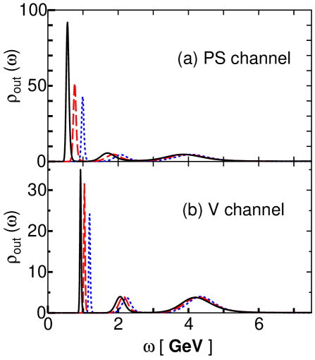
Figure 2: Reconstructed image $\rho_{out}(\omega)$ for the PS (a) and V (b) channels. The solid, dashed, and dotted lines are for $\kappa=$ 0.1557, 0.1545, and 0.153, respectively. For the PS (V) channel, $m_{0}$ is taken to be 2.0 (0.86). $\omega_{max}$ is 7.5 GeV in this figure and Fig.3.

As for the third bumps in Fig.2, the spectral “shape” is statistically not significant as is discussed in Fig.4, and they should rather be considered a part of the perturbative continuum instead of a single resonance. Fig.2 also shows that SPF decreases substantially above 6 GeV; MEM automatically detects the existence of the momentum cutoff on the lattice $\sim\pi/a$. It is expected that MEM with the data on finer lattices leads to larger ultraviolet cut-offs in the spectra. The height of the asymptotic form of the spectrum at high energy is estimated as

$$\mbox{}\rho_{{}_{V}}(\omega\simeq 6{\rm GeV})$$ (8)

$$\mbox{\hskip 14.22636pt}={1\over 4\pi^{2}}\left(1+{\alpha_{s}\over\pi}\right)\left({1\over 2\kappa Z_{{}_{V}}}\right)^{2}\simeq 0.86.$$

The first two factors are the $q\bar{q}$ continuum expected from perturbative QCD. The third factor contains the non-perturbative renormalization constant for the lattice composite operator. We adopt $Z_{{}_{V}}=0.57$ determined from the two-point functions at $\beta$ = 6.0 [11] together with $\alpha_{s}=0.21$ and $\kappa=0.1557$. Our estimate in eq.(4) is consistent with the high energy part of the spectrum in Fig.2(b) after averaging over $\omega$. We made a similar estimate for the PS channel using $Z_{{}_{PS}}=0.49$ [12] and obtained $\rho_{{}_{PS}}(\omega\simeq 6{\rm GeV})\simeq 2.0$. This is also consistent with Fig. 2(a). We note here that an independent analysis of the imaginary time correlation functions [2] also shows that the lattice data at short distance is dominated by the perturbative continuum.

In Fig.3(a) and (b), the results using the lattice kernel $K_{lat}$ are shown. $K_{lat}$ is obtained from the free boson propagator on the lattice. It reduces to $K_{cont}$ when $a\rightarrow 0$. The other parameters and boundary conditions are the same with Fig.2(a,b). The difference of Fig.2 and Fig.3 can be interpreted as a systematic error due to the finiteness of the lattice spacing $a$.

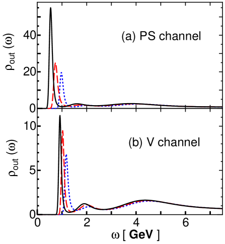
Figure 3: Same with Fig.2 except for the use of the lattice kernel $K_{lat}$.

5 Error analsis

The statistical significance of the reconstructed image can be studied by the following procedure [4]. Assuming that $P[A|DH\alpha m]$ has a Gaussian distribution around the most probable image $\hat{A}$, we estimate the error by the covariance of the image, $-\langle(\delta_{A}\delta_{A}Q)^{-1}\rangle_{A=\hat{A}}$, where $\delta_{A}$ is a functional derivative and $\langle\cdot\rangle$ is an average over a given energy interval. The final error for $A_{out}$ is obtained by averaging the covariance over $\alpha$ with a weight factor $P[\alpha|DHm]$. Shown in Fig.4 is the MEM image in the V channel for $\kappa=0.1557$ with errors obtained in the above procedure. The height of each horizontal bar is $\langle\rho_{out}(\omega)\rangle$ in each $\omega$ interval. The vertical bar indicates the error of $\langle\rho_{out}(\omega)\rangle$. The small error for the lowest peak in Fig.4 supports our identification of the peak with $\rho$. Although the existence of the non-vanishing spectral strength of the 2nd peak and 3rd bump is statistically significant, their spectral “shape” is either marginal or insignificant. Lattice data with better quality are called for to obtain better SPFs.

Figure 4: $\rho_{out}(\omega)$ in the $V$ channel for $\kappa=$ 0.1557 with error attached.

6 Summary

We have made a first serious attempt to reconstruct SPFs of hadrons from lattice QCD data. We have used MEM, which allows us to study SPFs without making a priori assumption on the spectral shape. The method works well for the mock data and actual lattice data. MEM produces resonance and continuum-like structures in addition to the ground state peaks. The statistical significance of the image can be also analyzed. Better data with finer and larger lattice will produce better images with smaller errors, and our study is a first attempt towards this goal.

There are many problems which can be explored by MEM combined with lattice QCD data. Some of the applications in the baryon excited states, hadrons at finite temperature, and heavy quark systems will be reported in future publications [13].

We appreciate MILC collaboration for their open codes for lattice QCD simulations, which has enabled this research. Our simulation was carried out on a Hitachi SR2201 parallel computer at Japan Atomic Energy Research Institute. M. A. (T. H.) was partly supported by Grant-in-Aid for Scientific Research No. 10740112 (No. 10874042) of the Japanese Ministry of Education, Science, and Culture.

References

- [1] E. V. Shuryak, Rev. Mod. Phys. 65,1 (1993).
- [2] M. -C. Chu, J. M. Grandy, S. Huang, and J. W. Negele, Phys. Rev. D 48, 3340 (1993).
- [3] Y. Nakahara, M. Asakawa and T. Hatsuda, hep-lat/9905034 (Phys. Rev. D in press).
- [4] See the review, M. Jarrell and J. E. Gubernatis, Phys. Rep. 269, 133 (1996).
- [5] R. N. Silver et al., Phys. Rev. Lett. 65, 496 (1990); W. von der Linden, R. Preuss, and W. Hanke, J. Phys. 8, 3881 (1996); N. Wu, The Maximum Entropy Method, (Springer-Verlag, Berlin, 1997).
- [6] D. B. Leinweber, Phys. Rev. D 51, 6369 (1995); D. Makovoz and G. A. Miller, Nucl. Phys. B468, 293 (1996); C. Allton and S. Capitani, Nucl. Phys. B526, 463 (1998); Ph. de Forcrand et al., Nucl. Phys. B (Proc. Suppl.) 63A-C, 460 (1998).
- [7] See e.g., J. Skilling, in Maximum Entropy and Bayesian Methods, ed. J. Skilling (Kluwer, London, 1989), pp.45-52; S. F. Gull, ibid. pp.53-71.
- [8] This formula is motivated by our lattice QCD data.
-
[9]
The MILC code ver. 5,
http://cliodhna.cop.uop.edu/~hetrick/milc . - [10] Y. Iwasaki et al., Phys. Rev. D 53, 6443 (1996); T. Bhattacharya et al., ibid. 6486.
- [11] L. Maiani and G. Martinelli, Phys. Lett. B178, 265 (1986).
- [12] M. Göckeler et al., Nucl. Phys. B544, 699 (1999).
- [13] M. Asakawa, T. Hatsuda and Y. Nakahara, in preparation.