Choice of Integrator in the Hybrid Monte Carlo Algorithm

Tetsuya Takaishi

Hiroshima University of Economics
Hiroshima 731-0192, JAPAN

1 Introduction

Inclusion of dynamical fermions is one of major difficulties in lattice QCD simulations since eventually one finds that the simulations require huge computational time. The standard algorithm for full QCD simulations is the hybrid Monte Carlo (HMC) algorithm[1]. While the basic idea of the HMC is a combination of molecular dynamics ( MD ) and Metropolis accept/reject steps, performance of its algorithm depends on tuning: matrix solver, parameter tuning, integration scheme etc. The matrix solver appears in the fermionic force calculations and takes the dominant time in the HMC simulations. The choice of an efficient matrix solver is an important subject to reduce CPU time [2]. Parameters ( $\beta$ and $\kappa$ etc ) of a MD Hamiltonian can be tuned so that the Metropolis acceptance rate increases [3].

One may choose any integrator for the MD step provided that the following two conditions are satisfied:

• area preserving

• time reversibility

Usually the ( 2nd order ) leapfrog integrator is used for the HMC. The leading integration errors are ${\cal O}(\Delta t^{3})$, where $\Delta t$ is the step size of an elementary MD step. Due to these errors the Hamiltonian is not conserved. Let $\Delta H$ be an energy violation at the end of a MD trajectory. To achieve the correct equilibrium a new configuration should be accepted by a global Metropolis test with a probability:

$$P\propto\min(1,\exp(-\Delta H)).$$ (1)

In order to have a high acceptance we may consider a more accurate integration scheme to reduce $\Delta H$. The multiple time scale method [4] which removes the dominant errors from the gauge part worked well. An idea [5] which controls the integration errors with an adaptive step size was also explored. However no practical gain appeared for QCD case [6]. One may employ a higher order integrator which has higher order integration errors in $\Delta t$. In general higher order integrators need more arithmetic operations than the 2nd order one. Therefore it is non-trivial whether the higher order integrators serve as an efficient speed-up source to the HMC. For QCD the 4th order one was studied on a $4^{4}$ lattice [4], and was found not to be efficient enough on such a small lattice.

When one compares higher order integrators, volume dependence must be considered. The average acceptance of an n-th order integrator is given by $\sim{\rm erfc}(cV^{1/2}\Delta t^{n})$, where $V$ is volume of the system considered and $c$ is a constant. To keep a constant acceptance, $\Delta t$ should scale $\sim 1/V^{1/2n}$. This scaling behaviour suggests that the higher order one will be efficient for a lattice bigger than a certain size. However we do not know the value of this lattice size. In this study we perform HMC simulations with 2nd, 4th and 6th order integrators and clarify which integrator is efficient for a given lattice. It now becomes feasible to perform a simulation on rather big lattices as $24^{3}\times 40-48$ lattices[7]. So it is worthwhile to study whether, on such lattices, the higher order integrators are more efficient than the standard leapfrog ( 2nd ) one.

In Sec.2 we describe the lattice QCD action used in our HMC simulations. In Sec.3 we describe the higher order integrators which we use. In Sec.4 we discuss the optimal efficiency, acceptance and step size of the HMC. In Sec.5 we give a criterion to compare various integrators. In Sec.6 we present our numerical results. Finally we summarize our results in Sec.7.

2 Lattice QCD action

We use the standard plaquette gauge action and two flavors Wilson fermion action [8]. The partition function is given by

$$Z=\int{\cal D}U\det[M(U)^{\dagger}M(U)]\exp(-S_{g}),$$ (2)

where $U$ stands for SU(3) link variables and

$$S_{g}=\frac{\beta}{3}\sum_{U_{p}}Tr(1-U_{p})$$ (3)

where $U_{p}$ stands for the plaquette and $\beta$ is the gauge coupling, and the Wilson fermion matrix $M(U)$ is given by

$$M_{ij}(U)=\delta_{i,j}+\kappa\sum_{\mu}[(\gamma_{\mu}-1)U_{i,\mu}\delta_{i,j+\mu}-(\gamma_{\mu}+1)U^{\dagger}_{i-\mu,\mu}\delta_{i,j+\mu}]$$ (4)

where $\kappa$ is the hopping parameter.

The expectation value of some operator $O(U)$ is given by

$$<O>=\int{\cal D}UO(U)\det[M(U)^{\dagger}M(U)]\exp(-S_{g})/Z.$$ (5)

Using pseudofermion fields $\phi$ we replace the determinant in Eq.(2) with a path-integral as

$$Z=\int{\cal D}U{\cal D}\phi^{*}{\cal D}\phi\exp[-S_{g}-\phi^{\dagger}(M(U)^{\dagger}M(U))^{-1}\phi].$$ (6)

Introducing momenta $p$ conjugate to link variables we define the Hamiltonian used in the HMC as

$$H=\frac{1}{2}p^{2}+S_{g}+\phi^{\dagger}(M(U)^{\dagger}M(U))^{-1}\phi$$ (7)

and the partition function will be

$$Z=\int{\cal D}U{\cal D}\phi^{*}{\cal D}\phi{\cal D}p\exp(-H),$$ (8)

which gives the same expectation values as that from Eq.(2).

3 Higher order integrators

In this section we describe higher order integrator scheme which we use for the present study. Let $H$ be a classical Hamiltonian,

$$H=\frac{1}{2}p^{2}+S(q)$$ (9)

where $q=(q_{1},q_{2},...)$ and $p=(p_{1},p_{2},...)$ are coordinate variables and conjugate momenta respectively, and $S(q)$ represents a potential term of the system. For simplicity we use scaler variables $p$ and $q$. The same discussion applies for QCD case where SU(3) link variables are used.

In the MD step we solve Hamilton’s equations,

$$\frac{dq_{i}}{dt}=\frac{\partial H}{\partial p_{i}}$$ (10)

$$\frac{dp_{i}}{dt}=-\frac{\partial H}{\partial q_{i}},$$ (11)

approximately by an appropriate integrator. In general these equations are not solvable analytically. Let $T_{MD}(\Delta t)$ be an elementary MD step with a time interval ( step size ) $\Delta t$, which evolves $(p,q)$ to $(p^{\prime},q^{\prime})$:

$$T_{MD}(\Delta t):(p,q)\longrightarrow(p^{\prime},q^{\prime}).$$ (12)

Requirements of the HMC to the integrator $T_{MD}(\Delta t)$ are (a) time reversible:

$$T_{MD}(-\Delta t):(p^{\prime},q^{\prime})\longrightarrow(p,q)$$ (13)

and (b) area preserving:

$$dpdq=dp^{\prime}dq^{\prime}$$ (14)

i.e. invariance of the measure. All integrators having the above requirements can be used for the HMC. The simplest integrator is the 2nd order leapfrog method which has been commonly used in the HMC of the current full QCD simulations. The 2nd order leapfrog scheme is explicitly written as

$$\left\{\begin{array}[]{ll}q(t+\frac{\Delta t}{2})&=q(t)+\frac{\Delta t}{2}p(t)\\ p(t+\Delta t)&=p(t)-\Delta t\frac{\partial S(q(t+\frac{\Delta t}{2}))}{\partial q}\\ q(t+\Delta t)&=q(t+\frac{\Delta t}{2})+\frac{\Delta t}{2}p(t+\Delta t).\end{array}\right.$$ (15)

While we start the integrator with variables $q$, alternatively we can use momenta $p$ for the starting variables. This 2nd order leapfrog integrator causes ${\cal O}(\Delta t^{3})$ integration error.

In order to construct a class of higher order integrators, it is convenient to use the Lie algebraic formalism [4, 11, 12, 14]. The Hamilton’s equation is written as

$$\frac{df}{dt}=\{f,H\}$$ (16)

where $f=p$ or $q$, and {,} stands for the Poisson bracket, i.e.

$$\{f,H\}=\sum_{i}(\frac{\partial f}{\partial q_{i}}\frac{\partial H}{\partial p_{i}}-\frac{\partial H}{\partial q_{i}}\frac{\partial f}{\partial p_{i}}).$$ (17)

Defining the linear ( Lie ) operator $L(H)$ as

$$L(H)f=\{f,H\},$$ (18)

we have the formal solution of the Hamilton’s equation:

$$f(t+\Delta t)=exp(\Delta tL(H))f(t).$$ (19)

Since $L(\cdot)$ is a linear operator, we have

$$L(H) = L(\frac{1}{2}p^{2})+L(S(q))$$ (20)

$$= T+V$$ (21)

where $T\equiv L(\frac{1}{2}p^{2})$ and $V\equiv L(S(q))$ stand for a kinetic and potential terms respectively. Using the Lie algebraic formalism, one finds that the 2nd leapfrog integrator corresponds to a decomposition of the exponential in Eq.(19) as

$$f(t+\Delta t) = \exp(\Delta t(T+V))f(t)$$ (22)

$$= \{exp(\frac{1}{2}\Delta tT)exp(\Delta tV)exp(\frac{1}{2}\Delta tT)+{\cal O}(\Delta t^{3})\}f(t).$$

Note that $T$ and $V$ do not commute with each other and ${\cal O}(\Delta t^{3})$ decomposition errors appear. An important observation here is that the order of the decomposition error coincides with that of the integration error.

An arbitrary order integrator can be found by decomposing the exponential with the desired order. In general, the exponential is decomposed as

$$exp(\Delta t(T+V))=\prod_{i}exp(c_{i}\Delta tT)exp(d_{i}\Delta tV)+{\cal O}(\Delta t^{n+1})$$ (23)

where $c_{i}$ and $d_{i}$ are determined so that the decomposition is correct up to ${\cal O}(\Delta t^{n})$. It is not obvious how to obtain such $c_{i}$ and $d_{i}$ in any order. Fortunately higher even-order integrators are known to be constructed from a combination of lower order integrators[11, 12, 13]. Let us call $G_{2nd}(\Delta t)$ the 2nd order decomposition ( or integrator),

$$G_{2nd}(\Delta t)\equiv exp(\frac{1}{2}\Delta tT)exp(\Delta tV)exp(\frac{1}{2}\Delta tT).$$ (24)

The 4th order integrator is given by a product of $three$ 2nd order integrators[10, 11, 12, 13],

$$G_{4th}(\Delta t)=G_{2nd}(a_{1}\Delta t)G_{2nd}(a_{2}\Delta t)G_{2nd}(a_{1}\Delta t)$$ (25)

where the coefficients $a_{i}$ are given by

$$a_{1}=\frac{1}{2-2^{1/3}},$$ (26)

$$a_{2}=-\frac{2^{1/3}}{2-2^{1/3}}.$$ (27)

This construction scheme is easily generalized for an arbitrary even-order one[11, 12, 13]. (2k+2)-th order integrator is given recursively by

$$G_{2k+2}(\Delta t)=G_{2k}(b_{1}\Delta t)G_{2k}(b_{2}\Delta t)G_{2k}(b_{1}\Delta t),$$ (28)

where the coefficient $b_{i}$ are

$$b_{1}=\frac{1}{2-2^{1/(2k+1)}}$$ (29)

$$b_{2}=-\frac{2^{1/(2k+1)}}{2-2^{1/(2k+1)}}.$$ (30)

While one can find an arbitrary higher even-order integrator with Eq.(28), the number of elementary steps ( 2nd order integrator ) grows with the order of the integrator as follows:

$$\#\mbox{ of 2nd order integrator}=\left\{\begin{array}[]{ll}1&2nd\\ 3&4th\\ 9&6th\\ \vdots&\vdots\\ 3^{n/2-1}&nth.\end{array}\right.$$ (31)

A bottleneck of the HMC for QCD is the force calculation $\partial S/\partial q$ which needs a large amount of computational time devoted to a matrix solver. Except for some small overhead, the computational cost of the HMC is proportional to the number of the force calculations. The 2nd order integrator contains one force calculation. Therefore the computational cost of the higher order algorithm can be counted by Eq.(31), which indicates that the cost grows rapidly with the order.

If one can find a higher order integrator consisting of fewer force calculations it may be useful for HMC. In Ref[12], such a higher order scheme is found numerically. In this study we also use the 6th order integrators of Ref[12] which consist of $seven$ 2nd order integrators instead of $nine$ as in Eq.(31). The 6th order integrators of Ref[12] are written as

$$G_{6th}(\Delta t) = G_{2nd}(w_{3}\Delta t)G_{2nd}(w_{2}\Delta t)G_{2nd}(w_{1}\Delta t)G_{2nd}(w_{0}\Delta t)$$ (32)

$$\times G_{2nd}(w_{1}\Delta t)G_{2nd}(w_{2}\Delta t)G_{2nd}(w_{3}\Delta t),$$

where values of $(w_{0},w_{1},w_{2},w_{3})$ are listed in Table 1.

Note that all the higher even-order integrators described here satisfy the time reversible and area preserving conditions since those are a product of the 2nd order integrators having the area preserving condition and are constructed in a symmetric way ( $G(\Delta t)G(-\Delta t)=1$ ) which yield the time reversible condition.

	Y1	Y2	Y3
$w_{1}$	-0.117767998417887e-1	-0.2132285222000144e+1	0.152886228424922e-2
$w_{2}$	0.235573213359357e+0	0.426068187079180e-2	-0.214403531630539e+1
$w_{3}$	0.784513610477560e+0	0.143984816797678e+1	0.144778256239930e+1

Table 1: Parameter sets (Y1-Y3) of the 6th order integrators by Yoshida [12]. $w_{0}$ is given by $w_{0}=1-w_{1}-w_{2}-w_{3}$.

4 Optimal efficiency, acceptance and step size

In this section we introduce an efficiency function which characterizes the speed of algorithm and derive formulae for the optimal acceptance and step size which define the optimal efficiency.

We define the efficiency function $E_{ff}$ by a product of step size $\Delta t$ and acceptance $P_{acc}(\Delta t)$:

$$E_{ff}(\Delta t)=P_{acc}(\Delta t)\Delta t.$$ (33)

High $E_{ff}$ results in fast Markov step when producing configurations. A particular length of trajectory does not affect $E_{ff}$ since the acceptance stays almost constant for any trajectory length longer than a certain characteristic length[15]. This is a feature of the symplectic type integrator [14]. We fix the trajectory length to the unit length (=1) which is sufficiently longer than the characteristic length for the present study.

The acceptance decreases as $\Delta t$ increases. In both limits of $\Delta t=0$ and $\infty$, $E_{ff}$ goes to zero. We expect that $E_{ff}$ has one maximum at a certain $\Delta t$, which we call optimal step size $\Delta t_{opt}$.

Using $\Delta t_{opt}$ we define the optimal acceptance $(P_{acc})_{opt}$:

$$(P_{acc})_{opt}=P_{acc}(\Delta t_{opt}),$$ (34)

and the optimal efficiency $(E_{ff})_{opt}$:

$$(E_{ff})_{opt} = \max(E_{ff}(\Delta t))=E_{ff}(\Delta t_{opt})$$ (35)

$$= (P_{acc})_{opt}\Delta t_{opt}.$$ (36)

When we have $(E_{ff})_{opt}$ the maximum speed of the algorithm is achieved. Comparison among various integrators will be done with this $(E_{ff})_{opt}$. At this stage, however, it is not obvious how to obtain $(E_{ff})_{opt}$ easily from Monte Carlo (MC) simulations. In the following consideration, we show that one coefficient governs $(E_{ff})_{opt}$ and it is easily obtainable from a MC simulation.

At large volumes, the average acceptance with an average energy difference is evaluated as [15]

$$\langle P_{acc}\rangle = {\rm erfc}(\frac{1}{2}\langle\Delta H\rangle^{1/2}).$$ (37)

Although Eq.(37) is applicable for the whole range of the acceptance, i.e. $1\geq\ \langle P_{acc}\rangle\geq 0$, we are not interested in low acceptance with which the algorithm may not be efficient. Typically we may need $\langle P_{acc}\rangle>50\%$. Instead of Eq.(37) we propose a simple exponential type formula:

$$\langle P_{acc}\rangle=\exp(-\frac{2}{\sqrt{\pi}}\langle\frac{1}{8}\Delta H^{2}\rangle^{1/2}).$$ (38)

In the limit of $\langle\Delta H\rangle\rightarrow 0$, Eq.(38) coincides with Eq.(37) ( See Appendix ). Even if $\langle\Delta H\rangle$ is not small enough ( $\langle\Delta H\rangle\simeq 1$ ), from numerical tests we confirm that Eq.(38) is a good approximation to the exact value. Fig.1 shows comparison of MC results and values from Eq.(38). Fig.2 shows a normalized error [(MC$-$Eq.(38))/Eq.(38)] as a function of $\langle\Delta H^{2}\rangle^{1/2}$. From the comparison of MC results and Eq.(38) we notice that Eq.(38) agrees quite well with the MC results within $5\%$ error up to $\langle\Delta H^{2}\rangle^{1/2}\leq 3$, which roughly corresponds to $\langle P_{acc}\rangle\geq 20\%$. Therefore we adopt Eq.(38) as our formula for $\langle P_{acc}\rangle$.

Let us now discuss $\Delta t$ dependence of $\langle\Delta H^{2}\rangle^{1/2}$ which appears in Eq.(38). The 2nd order integrator causes ${\cal O}(\Delta t^{3})$ integration errors after an elementary MD step. From the discussion of Ref.[15], however, $\Delta H\sim\Delta t^{2}$ rather than $\sim\Delta t^{3}$. This comes from the fact that $\Delta H$ does not grow with the trajectory length ( = the number of elementary MD steps $\times\Delta t$ ). Using $\langle\Delta H\rangle\approx\frac{1}{2}\langle\Delta H^{2}\rangle$ which is expected from Creutz’s equality[16] $\langle\exp(-\Delta H)\rangle=1$ at small $\Delta H$, we obtain

$$\langle\Delta H\rangle\sim\langle\Delta H^{2}\rangle\sim V\Delta t^{4}$$ (39)

where $V$ is the volume of the system. When we apply the same discussion for the n-th order integrator we have

$$\langle\Delta H^{2}\rangle\sim V\Delta t^{2n}.$$ (40)

Thus,

$$\langle\Delta H^{2}\rangle^{1/2}\sim V^{1/2}\Delta t^{n}.$$ (41)

For our later use we rewrite Eq.(41) as

$$\langle\Delta H^{2}\rangle^{1/2}=C_{n}V^{1/2}\Delta t^{n}+{\cal O}(\Delta t^{n+1}),$$ (42)

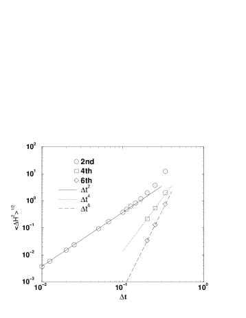
Figure 3: $\langle\Delta H^{2}\rangle^{1/2}$ for the 2nd, 4th and 6th order integrators as a function of $\Delta t$. The simulations ( quenched QCD ) were done on a $4^{4}$ lattice at $\beta=5.0$. Three lines in the figure are shown to guide the eye.

where $C_{n}$ is a Hamiltonian ( model ) dependent coefficient, which is not known a priori. We checked Eq.(42) by MC simulations, as shown in Fig.3. When $\Delta t$ is not too large, Eq.(42) holds.

Here we comment on the 6th order integrator. In the MC simulations for Fig.3, the standard construction scheme of Eq.(28) was used. We have other 6th order integrators defined by Eq.(32) which have less computational cost. These have the same power of $\Delta t$ to the leading term. The proportional coefficient $C_{n}$ ( here $n=6$ ), however, can be different for each 6th order integrator. We numerically calculated $C_{n}$ of each integrator using quenched QCD and quenched Schwinger ( QED₂ ) models. Fig.4 shows $\langle\Delta H^{2}\rangle^{1/2}$ as a function of $\Delta t$, where Stand indicates the standard construction scheme of Eq.(28). Others are from Eq.(32). The most efficient one is the integrator Y1 in Table 1, of which $C_{n}$ is roughly a factor of ten smaller than others. The results from others are more or less same. The same conclusion is also applied for the Schwinger model as shown in Fig.5. It seems that Y1 is always the most efficient one. Thus in the following analysis we use Y1 as our 6th order integrator.

Using Eq.(42) without higher order terms, we find a formula for the average acceptance, instead of Eq.(38), as

$$\langle P_{acc}\rangle=\exp(-\widetilde{C}_{n}V^{\frac{1}{2}}\Delta t^{n}),$$ (43)

where $\widetilde{C}_{n}=C_{n}/\sqrt{2\pi}$. Using this expression, we can easily obtain the optimal step size as

$$\Delta t_{opt}=\sqrt[n]{\frac{1}{n\widetilde{C}_{n}V^{\frac{1}{2}}}}.$$ (44)

Substituting this result to Eq.(34) we obtain the optimal acceptance as

$$\langle P_{acc}\rangle_{opt} = \exp(-\frac{1}{n})$$ (45)

$$= \left\{\begin{array}[]{ll}0.61&\mbox{2nd}\\ 0.78&\mbox{4th}\\ 0.85&\mbox{6th}.\end{array}\right.$$ (49)

Finally from Eq.(44) and Eq.(45) we obtain the optimal efficiency of the n-th order integrator:

$$(E_{ff})_{opt}^{n-th}=\exp(-\frac{1}{n})\sqrt[n]{\frac{1}{n\widetilde{C}_{n}V^{\frac{1}{2}}}},$$ (50)

and find that Eq.(50) is governed by only one unknown $\widetilde{C}_{n}$.

The result of Eq.(45) suggests that there exists an optimal acceptance depending only on the order of the integrator, not on the model. The optimal acceptance increases with increase of the order of the integrator. We verify this feature by MC simulations. First we show results of QCD for 2nd order one and then that of quenched Schwinger model ( QED₂ ) for 2nd,4th and 6th order ones. The Schwinger model is used to reduce the CPU time.

In Fig.6 results for the 2nd order integrator from three parameter sets among different $\beta=(5.3,5.0,0.0)$, $\kappa=(0,0.2)$ and volume $V=(6^{4},4^{4})$ are plotted. For all the cases the optimal acceptance locates around a value between $60-70\%$ which is in good agreement with the analytic estimate ( 61% ) of Eq.(49). The results with different lattice volume compare lattice size dependence on $(E_{ff})_{opt}$. Since QCD is a 4-dimensional model ( $V=L^{4}$ where $L$ is lattice size ) we find $(E_{ff})_{opt}\sim 1/L$ for the 2nd order integrator. The MC results from $4^{4}$ and $6^{4}$ lattices with slightly different $\beta$ agree with this expectation, i.e. $(E_{ff})_{opt}[4^{4}]/(E_{ff})_{opt}[6^{4}]\sim 1.5$ ( See Fig.6 ).

Fig.7 compares $(E_{ff})$ among 2nd, 4th and 6th integrators. It is clearly seen that the optimal acceptance increases with increase of the order, which is again in agreement with Eq.(49).

5 Comparison of various integrators

In this section we give a criterion to compare various integrators. Let us consider the n-th and m-th order integrators ($n>m$). As seen in the previous section, each integrator has the optimal efficiency given by Eq.(50). In order to have a better performance for the n-th order integrator than for the m-th one, the optimal efficiency of the n-th one should be larger than that of the m-th one. Furthermore we must consider the cost to perform the higher order one since the higher order one needs more arithmetic operations. Thus the following equation should be satisfied,

$$(E_{ff})^{n-th}_{opt}>k_{nm}(E_{ff})^{m-th}_{opt}$$ (51)

where $k_{nm}$ is a relative cost factor needed to implement the n-th order integrator against the m-th one.

Substituting Eq.(50) to Eq.(51), we obtain

$$\exp(-\frac{1}{n})\sqrt[n]{\frac{1}{n\widetilde{C}_{n}V^{\frac{1}{2}}}}>k_{nm}\exp(-\frac{1}{m})\sqrt[m]{\frac{1}{m\widetilde{C}_{m}V^{\frac{1}{2}}}}.$$ (52)

Rewriting Eq.(52), we obtain an expression for volume size with which the n-th order integrator performs better than the m-th order one,

$$V^{\frac{n}{2}-\frac{m}{2}}>(k_{nm}\exp(-\frac{1}{m}+\frac{1}{n}))^{nm}\left(\frac{1}{m\widetilde{C}_{m}}\right)^{n}(n\widetilde{C}_{n})^{m}.$$ (53)

In the present study we compare (A): 2nd and 4th order integrators, and (B): 4th and 6th order integrators.

(A): 4th order versus 2nd order

In this case $n=4$ and $m=2$. From Eq.(31) we find the relative cost is $k_{4,2}=3$. Substituting $k_{4,2}=3$ into Eq.(53) we obtain

$$V^{\frac{1}{2}}>(3\exp(-\frac{1}{4}))^{4}\left(\frac{1}{\widetilde{C}_{2}}\right)^{2}\widetilde{C}_{4}.$$ (54)

(B): 6th order versus 4th order

In this case $n=6$ and $m=4$. Since we use the scheme of Eq.(32), the relative cost $k_{6,4}$ is $7/3$. Thus we obtain

$$V^{\frac{1}{2}}>\left(\frac{7}{3}\exp(-\frac{1}{12})\right)^{12}\left(\frac{1}{4\widetilde{C}_{4}}\right)^{3}\left(6\widetilde{C}_{6}\right)^{2}.$$ (55)

6 Lattice size for higher order integrator

Now we come to the stage of determination of lattice sizes which are suitable for the higher order integrators. Eqs.(54)-(55) determine regions where the higher order integrators perform better than the lower one. In practice we solve Eqs.(54)-(55) equating both sides of the equations. The solutions ( in lattice size ) form a boundary which separates two regions: higher order and lower order preferred regions. Unknown $\widetilde{C}_{n}$ should be obtained from numerical simulations. We choose a small enough $\Delta t$ and compute $\langle\Delta H^{2}\rangle^{1/2}$. Applying Eq.(42) for $\langle\Delta H^{2}\rangle^{1/2}$ we extract $C_{n}(=\sqrt{2\pi}\widetilde{C}_{n})$.

First we study quenched QCD where $C_{n}$ are determined as a function of $\beta$, and then go to full QCD with two flavors of Wilson fermions where $C_{n}$ are a function of $\kappa$.

6.1 Quenched QCD

Numerical simulations were performed on a $4^{4}$ lattice. Fig.8 shows $C_{n}$ as a function of $\beta$. We also used an $8^{4}$ lattice at several $\beta$ to check the volume dependence appearing in Eq.(42). The values of $C_{n}$ obtained from both lattices were same, which suggests that we can get reliable values of $C_{n}$ on the lattice of this size.

Fig.9 shows results of the boundaries determined from Eqs.(54)-(55). The circle symbols form a boundary which separates the 2nd order preferred region ( lower region ) and the 4th order preferred one ( upper region ). Similarly the squares separate the 4th order one ( lower ) and the 6th order one ( upper ).

The boundary between the 2nd order one and the 4th order one (B2-4) increases as $\beta$ increases and reaches a plateau at $\beta\sim 3.0$. The corresponding lattice size is about $\sim 10^{4}$. On the other hand the boundary between the 4th and the 6th one (B4-6) decreases with $\beta$. At $\beta\sim 5.0$ the lattice size on B4-6 is about $20^{4}$. At $\beta\sim 5.0$, the 4th order integrator becomes efficient for $L>10$ and the 6th order one for $L>20$.

6.2 Full QCD

We use a model with two flavors of Wilson fermions. To consider fermion dynamics only we take $\beta=0$ and simulate the model with varying $\kappa$. An advantage of taking $\beta=0$ is that the critical kappa is known analytically, i.e. $\kappa_{c}=0.25$. Using the critical kappa the quark mass at $\beta=0$ is defined by $\widetilde{m}_{q}=m_{q}a=\ln(1+\frac{1}{2}(1/\kappa-1/\kappa_{c}))$.

Fig.10 shows $C_{n}$ as a function of quark mass. The simulations were done on a $4^{4}$ lattice. We see that $C_{n}$ behaves as a power of quark mass, i.e. $C_{n}\propto\widetilde{m}_{q}^{-\alpha}$. Using three data at small $\widetilde{m}_{q}(\kappa=0.215,0.225,0.230)$, $\alpha$ are estimated to be $\alpha\sim 1.55(8),4.58(11),7.65(11)$ for 2nd, 4th and 6th order respectively. For the 2nd order, this result is consistent with that of the staggered fermion[15]: $\alpha\approx 1.5$.

Fig.11 shows results of B2-4 and B4-6. Both B2-4 and B4-6 increase with decreasing quark mass. We estimate quark mass dependence of the boundaries as: B2-4 $\propto C_{4}^{1/2}/C_{2}\sim\widetilde{m}_{q}^{-0.74}$ and B4-6 $\propto C_{6}/C_{4}^{3/2}\sim\widetilde{m}_{q}^{-0.73}$. For both, values of the power are negative, which means that at small quark masses, the lattice size needed to have a gain with the higher order integrator increases. If we stay at $L<24(40)$ which is a lattice size available for the current ( or near-future ) full QCD simulations, the 4th order integrator can be efficient for $\widetilde{m}_{q}>0.3(0.1)$. The chiral limit ( $m_{q}\rightarrow 0$ ) is the primary interesting case in full QCD simulations. Therefore our results show that the standard leapfrog ( 2nd order ) integrator is the best one for most full QCD simulations except for heavy quarks.

For comparison we also give results of the Schwinger model with staggered quarks at $\beta=0.0$. Fig.12 shows $C_{n}$ as a function of staggered quark mass. The behaviour of $C_{n}$ is similar to that of the full QCD case, i.e. $C_{n}\propto\widetilde{m}_{q}^{-\alpha}$ : $\alpha$ is estimated to be 1.36(9), 3.36(27) and 5.41(23) for 2nd, 4th and 6th integrators respectively. The estimation is based on the data at small quark masses. Fig.13 shows B2-4 and B4-6. Here note that $V=L^{2}$ since the Schwinger model is a 2 dimensional model.

Although we considered $\beta=0.0$ case only, at finite $\beta$ we expect the similar diagram as in Fig.11 for small $m_{q}a$. The reason is the following. The fermionic force is expected to become dominant over the gauge force at small $m_{q}a$. In such a case, the integration error from the fermionic part also becomes dominant at small $m_{q}a$. As seen in Fig.8 all $C_{n}$ of quenched QCD at $\beta\sim 5.0$ are less than 10. On the other hand all $C_{n}$ at $m_{q}a<0.2$ are bigger than 100. Therefore the naive expectation is that the dominant contribution to $\langle\Delta H^{2}\rangle^{1/2}$ at small $m_{q}a$ comes from the fermionic part and values of $C_{n}$ at small $m_{q}a$ may not drastically change from that of $C_{n}$ at $\beta=0.0$. No change of $C_{n}$ results in no change of the boundaries ( B2-4 and B4-6 ).

We might also expect that the multiple time scale method [4] does not work for small $m_{q}a$ since it integrates finely only the gauge part and the dominant error from the fermionic part remains big at small quark masses.

To justify the above expectations, we calculate $C_{n}$ at various $\beta$ and illustrate how the dominant contribution to $\langle\Delta H^{2}\rangle^{1/2}$ comes from the fermionic part. For this purpose we choose the Schwinger model with staggered fermions, which requires less CPU time. Fig.14 shows $C_{2}$ versus $m_{q}a$ at $\beta=0.0$, 0.5 and 1.0. At large $m_{q}a$, the fermionic contributions are expected to be small and, in the limit of $m_{q}a\rightarrow\infty$ the values of $C_{n}$ go to those of quenched ones. In contrast to the situation at large $m_{q}a$, as $m_{q}a$ goes to small quark masses, values of $C_{2}$ at finite $\beta$ become similar to those of $C_{2}$ at $\beta=0.0$, which shows that the fermionic contribution becomes dominant and the values of $\beta$ are less important. We observed similar results for the higher order integrators. Therefore we deduce the similar result to that at $\beta=0.0$.

7 Summary

We have investigated higher order integrators for HMC with a criterion which compares among various integrators. The criterion is governed by one unknown parameter which is easily obtainable from a MC simulation. We have made comparison with quenched and full QCD models.

For quenched QCD the 4th order integrator performs better than the 2nd one for a lattice with size $L>10$ at $\beta\sim 5.0$. Of course usually the HMC is not used for quenched QCD simulations. If one uses a complicated action which is not implemented effectively with a local update algorithm the HMC with a higher order integrator could be an efficient algorithm for its simulation.

For full QCD the higher order integrators can be efficient only for large $m_{q}a$. For instance, on a currently accessible big lattice ( $L\sim 24$ ) the 4th order one performs better than the 2nd order one only for $m_{q}a>0.3$, which is out of interest for most full QCD simulations. Thus the 2nd order one is the best one for the current full QCD simulations.

The higher order integrators are turned out to be uninteresting at low $\beta$ ( Fig.9 ) and small $m_{q}a$ ( Fig.11 ). This may be due to the fact that QCD becomes more perturbative (i.e. close to a integrable system) at high $\beta$ and large $m_{q}a$. The Hamilton’s equations can be effectively integrated with higher order integrators in perturbative region. On the other hand, at low $\beta$ and small $m_{q}a$ (in non-perturbative region), the higher order integrators may not be efficient enough.

The optimal acceptance strongly depends on the order of the integrator. An interesting case is the 2nd order one, where the optimal acceptance is measured to be around 60-70% ( analytically estimated to be 61% ). This indicates that a very high acceptance like 80-90% or more is not required for the HMC with the 2nd order integrator. We suggest to take an acceptance around 60-70% for 2nd order HMC simulations of any model.

We have not considered finite temperature case. Ref.[15] found that quark mass dependence of the coefficient ( here $\sim C_{2}$ ) is very weak in the finite temperature phase. If this is also true for the higher order integrators the boundaries may not increase rapidly with decreasing quark mass as fast as in the zero temperature case.

ACKNOWLEDGMENTS

The author would like to thank Ph. de Forcrand for valuable comments and helpful discussions. He is also grateful to A.Nakamura and O.Miyamura for discussions. This work was supported in part by Hiroshima University of Economics, and by the Grant in Aid for Scientific Research by the Ministry of Education (No.11740159).

APPENDIX

When the argument $x$ is small, the error function erfc($x$) is approximated as follows.

$${\rm erfc}(x) = 1-{\rm erf}(x)$$ (56)

$$= 1-\frac{2}{\sqrt{\pi}}\int^{x}_{0}dte^{-t^{2}}$$

$$= 1-\frac{2}{\sqrt{\pi}}(x+x^{2}+...)$$

$$\approx \exp(-\frac{2}{\sqrt{\pi}}x).$$

Thus, using $\langle\Delta H\rangle\approx\frac{1}{2}\langle\Delta H^{2}\rangle$ at small $\langle\Delta H\rangle$, Eq.(37) is approximated as

$$\langle P_{acc}\rangle = {\rm erfc}(\frac{1}{2}\langle\Delta H\rangle^{1/2})$$ (57)

$$\approx {\rm erfc}(\langle\frac{1}{8}\Delta H^{2}\rangle^{1/2})$$ (58)

$$\approx \exp(-\frac{1}{\sqrt{2\pi}}\langle\Delta H^{2}\rangle^{1/2}).$$ (59)

Figure 1: Comparison of the average acceptance between $\exp(-\langle\Delta H^{2}\rangle^{1/2}/\sqrt[]{2\pi})$ and MC results as a function of $\langle\Delta H^{2}\rangle^{1/2}$.

Figure 2: Difference between $\exp(-\langle\Delta H^{2}\rangle^{1/2}/\sqrt{2\pi})$ and MC results. Error is defined by (MC data - $x$)/$x$, where $x=\exp(-\langle\Delta H^{2}\rangle^{1/2}/\sqrt{2\pi})$.

Figure 4: Comparison of $\langle\Delta H^{2}\rangle^{1/2}$ among various 6th order integrators as a function of $\Delta t$. Stand indicates the standard construction scheme of Eq.(28). Y1-Y3 indicate Yoshida’s construction scheme. The quenched QCD simulations were done on a $4^{4}$ lattice at $\beta=5.0$.

Figure 5: Same as in Fig.4 but for quenched Schwinger simulations on an $8^{2}$ lattice at $\beta=1.0$.

Figure 6: The efficiency $E_{ff}$ of the 2nd order integrator as a function of the average acceptance.

Figure 7: Comparison of the efficiency $E_{ff}$ among the 2nd, 4th and 6th order integrators for the quenched Schwinger model as a function of the average acceptance. Simulations were done on a $32^{2}$ lattice at $\beta=10.0$.

Figure 8: $C_{n}$ for quenched QCD as a function of $\beta$.

Figure 9: Results of the boundaries B2-4 and B4-6 for quenched QCD. Lines are shown to guide the eye.

Figure 10: $C_{n}$ for full QCD as a function of $m_{q}a$, where $m_{q}a=\ln(1+\frac{1}{2}(1/\kappa-1/\kappa_{c}))$.

Figure 11: Results of the boundaries B2-4 and B4-6 for full QCD at $\beta=0.0$. The dashed line is an anticipated boundary of B2-4.

Figure 12: $C_{n}$ for the Schwinger model with staggered quarks at $\beta=0.0$.

Figure 13: Results of the boundaries B2-4 and B4-6 for Schwinger model with staggered quarks at $\beta=0.0$.

Figure 14: $C_{2}$ versus $m_{q}a$ for the Schwinger model with staggered quarks at $\beta=0.0$, 0.5 and 1.0.

References

- [1] S.Duane, A.D.Kennedy, B.J.Pendleton and D.Roweth, Phys. Lett. B195, 216 (1987); S.Gottlieb, W.Liu, D.Toussaint, R.L.Renken and R.L.Sugar, Phys. Rev. D 35, 2531 (1987)
- [2] e.g. A.Frommer, Nucl. Phys. B ( Proc. Suppl. ) 53, 120 (1997)
- [3] R.Gupta,G.W.Kilcup and S.R.Sharpe, Phys. Rev. D 38, 1278 (1988)
- [4] J.C.Sexton, D.H.Weingarten, Nucl. Phys. B380, 665 (1992)
- [5] Ph. de Forcrand, Nucl. Phys. B ( Proc. Suppl. ) 47, 228 (1996)
- [6] Ph. de Forcrand and T.Takaishi, Phys. Rev. E 55, 3658 (1997)
- [7] TL-Collaboration, Nucl. Phys. B (Proc. Suppl.) 53, 222 (1997); CP-PACS Collaboration, Nucl. Phys. B (Proc. Suppl.) 73, 192 (1999)
- [8] K.G.Wilson, Phys. Rev. D 10, 2445 (1974); in New Phenomena in Subnuclear Physics, ed. A.Zichichi, 69 (New York, Plenum, 1975)
- [9] R.Gupta, A.Patel, C.F.Baillie, G.Guralnik, G.W.Kilcup and S.R.Sharpe, Phys. Rev. D 40, 2072 (1989)
- [10] M.Campostrini and P.Rossi, Nucl. Phys. B329, 753 (1990)
- [11] M.Creutz and A.Gocksch, Phys. Rev. Lett. 63, 9 (1989)
- [12] H.Yoshida, Phys. Lett. A150, 262 (1990)
- [13] M.Suzuki, Phys. Lett. A146, 319 (1990)
- [14] B.Gladman, M.Duncan and J.Candy, Celestial Mechanics 52, 221 (1991)
- [15] S.Gupta, A.Irbäck, F.Karch and B.Petersson, Phys. Lett. B242, 437 (1990)
- [16] M.Creutz, Phys. Rev. D 38, 1228 (1988) 1228