Crossing the c=1 Barrier in 2d Lorentzian Quantum Gravity

Abstract:

In an extension of earlier work we investigate the behaviour of two-dimensional Lorentzian quantum gravity under coupling to a conformal field theory with $c>1$. This is done by analyzing numerically a system of eight Ising models (corresponding to $c\!=\!4$) coupled to dynamically triangulated Lorentzian geometries. It is known that a single Ising model couples weakly to Lorentzian quantum gravity, in the sense that the Hausdorff dimension of the ensemble of two-geometries is two (as in pure Lorentzian quantum gravity) and the matter behaviour is governed by the Onsager exponents. By increasing the amount of matter to 8 Ising models, we find that the geometry of the combined system has undergone a phase transition. The new phase is characterized by an anomalous scaling of spatial length relative to proper time at large distances, and as a consequence the Hausdorff dimension is now three. In spite of this qualitative change in the geometric sector, and a very strong interaction between matter and geometry, the critical exponents of the Ising model retain their Onsager values. This provides evidence for the conjecture that the KPZ values of the critical exponents in 2d Euclidean quantum gravity are entirely due to the presence of baby universes. Lastly, we summarize the lessons learned so far from 2d Lorentzian quantum gravity.

1 Introduction

It may come as a surprise to practitioners of two-dimensional gravity that there is more than one way of constructing a viable quantum theory by path-integral methods, and that there is indeed “life beyond Liouville gravity”. The new, alternative theory of 2d quantum gravity in question was first constructed as the continuum limit of an exactly soluble model of dynamically triangulated two-geometries [1], which could be interpreted as representing Lorentzian geometries with a causal structure and a preferred time direction. It has recently been shown that there is a whole universality class of such Lorentzian models, some of which are obtained by adding a curvature term to the gravity action or by using building blocks different from triangles in the construction of geometries [2].

An investigation of Lorentzian gravity coupled to Ising spins led to the conclusion that in spite of strong fluctuations of the underlying geometries, the critical matter behaviour in the coupled system is governed by the Onsager exponents [3] (which one also finds for the Ising model on a fixed, regular lattice). This immediately raises the following questions: If we continue to add matter to the system, do we eventually observe a qualitative change in the behaviour of geometry and/or matter? Is there an analogue of the $c\!=\!1$ barrier of Liouville quantum gravity beyond which the combined gravity-matter system degenerates? We address these and related issues below, by studying numerically 8 Ising models (corresponding to a $c\!=\!4$ conformal field theory) coupled to Lorentzian quantum gravity.

In order to set the stage for our present investigation, let us recall some salient features of the Lorentzian gravity model [1, 4]. One idea behind the formulation of such a model is to take the Lorentzian structure seriously within a path-integral approach and in this way bridge the gap between the canonical quantization and the (Euclidean) path-integral formulation of gravity. The Lorentzian aspects of the model are two-fold: compared with the Euclidean case, the state sum is taken over a restricted class of triangulated two-geometries, namely, those which are generated by evolving a one-dimensional spatial slice and allow for the introduction of a causal structure. Secondly, the Lorentzian propagator is obtained by a suitable analytic continuation in the coupling constant. During time evolution, we do not permit the spatial slice to split into several components (i.e. change its topology), because the resulting space-time geometry would not be compatible with our discrete notion of causality. (In a continuum picture, the local lightcone structure associated with a Lorentzian metric must necessarily become degenerate at such branching points.) This is exactly the situation described by usual canonical (quantum) gravity.

In the pure gravity model, the loop-loop correlator and various geometric properties can be calculated exactly and compared to Euclidean 2d quantum gravity, as given by Liouville gravity or 2d quantum gravity defined by dynamical triangulations or matrix models. The two models turn out to be inequivalent. For example, the Hausdorff dimension of the Lorentzian quantum geometry is $d_{H}=2$, indicating a much smoother behaviour than that of the Euclidean case where $d_{H}\!=\!4$. The difference between the fractal structures of Lorentzian and Euclidean quantum gravity can be traced to the absence or presence of so-called baby universes. These are outgrowths of the geometry taking the form of branchings-over-branchings, which are known to dominate the typical geometry contributing to the Euclidean state sum. Such branchings and associated topology changes with respect to the preferred spatial slicing are absent from the histories contributing to the Lorentzian state sum.

Baby universes, i.e. discrete evolution moves resulting in spatial topology changes may be re-introduced by hand in the Lorentzian formulation (if one is willing to give up causality). This corresponds to “switching on” an additional term in the differential equation for the propagator, in such a way that the scaling limit must be modified in order to produce well-defined continuum physics.

A further difference between 2d Lorentzian and Euclidean gravity is revealed by coupling them to conformal matter. In the Euclidean case this is governed by the famous KPZ scaling relations. They describe how the critical exponents of a conformal field theory change when it is coupled to Euclidean quantum gravity, and how the entropy exponent $\gamma_{str}$ for two-geometries (the so-called string susceptibility) changes due to their coupling to the conformal matter fields.

In 2d Lorentzian gravity, the continuum limit of the quantum geometry was found to be unchanged under coupling to a $c\!=\!1/2$ conformal field theory, in the form of an Ising model at its critical point. The Hausdorff dimension remains equal to two, and an appropriately rescaled distribution of spatial volumes coincides with the distribution found in pure Lorentzian gravity. In addition, the values of the critical exponents of the Ising model agree with those of the Ising model on a regular lattice. In other words, coupling the Ising model to Lorentzian gravity does not affect the nature of its (second-order) phase transition. Summarizing, one may say that the coupling between $c\!=\!1/2$ conformal matter and geometry in Lorentzian quantum gravity is weak.

To avoid a frequent misunderstanding, we must emphasize that this is not a trivial consequence of the fact that $d_{H}\!=\!2$ in Lorentzian quantum gravity. Although a flat space-time implies $d_{H}\!=\!2$ for the Hausdorff dimension, the converse is by no means true. In fact, the geometry does fluctuate strongly in Lorentzian gravity, as was demonstrated in [1, 3]. There are other examples to illustrate that the Hausdorff dimension is only a very rough measure of geometry. Consider 2d Euclidean quantum gravity coupled to conformal field theories with $c>1$: in these models the geometry fluctuates so wildly that the two-dimensional surfaces are torn apart and degenerate into so-called branched polymers, which again have $d_{H}=2$, the same as for smooth surfaces!

An important conclusion one can draw from the results obtained in [3] is that the strong coupling between Euclidean quantum gravity and conformal matter is directly caused by the presence of baby universes. Various qualitative arguments have been put forward in the past to support this idea, which is of course not new. However, one never had a model which prohibited the creation of baby universes, and which could be used to verify explicitly that the coupling between geometry and matter in this case is weak. The observed weak-coupling behaviour in the Lorentzian model opens up the intriguing possibility that one might be able to cross the $c\!=\!1$ barrier in Lorentzian 2d quantum gravity coupled to matter. This is the issue we will study numerically in the remainder of this article, by coupling eight Ising models to Lorentzian quantum gravity, corresponding at the critical point of the combined system to a $c\!=\!4$ conformal field theory.

2 Coupling gravity to multiple Ising spins

In our previous work [1] we have defined the two-loop function of Lorentzian 2d gravity as the state sum

$$G(\lambda,t)=\sum_{T\in{\cal T}_{t}}e^{-\lambda N_{T}},$$ (1)

where the summation is over all triangulations $T$ of cylindrical topology with $t$ time-slices, $N_{T}$ counts the number of triangles in the triangulation $T$, and $\lambda$ is the bare cosmological constant. Since we are primarily interested in the bulk behaviour of the gravity-Ising system, we use periodic boundary conditions by identifying the top and bottom spatial slices of the cylindrical histories contributing to the state sum (1). Clearly this is not going to affect the local properties of the model. A geometry characterized by a toroidal triangulation $T$ of volume $N_{T}$ contains $N_{T}$ time-like links, $N_{T}/2$ space-like links, $N_{T}/2$ vertices and $3N_{T}/2$ nearest-neighbour pairs.

The partition function of $n$ Ising models coupled to 2d Lorentzian quantum gravity is given by

$$G(\lambda,t,\beta)=\sum_{T\in{\cal T}_{t}}e^{-\lambda N_{T}}Z_{T}^{n}(\beta),$$ (2)

where $T$ is now a triangulation with toroidal topology. The partition function for a single Ising model on the triangulation $T$ is denoted by $Z_{T}(\beta)$, where the spins are located at the vertices of $T$ and $\beta$ is the inverse temperature of the Ising model.

On a fixed lattice there are no interactions among the $n$ Ising spin copies if the partition function is simply taken as the $n$-fold product of $Z(\beta)$ for a single Ising model. In the presence of gravity, given by the definition (2), the situation is different. Although the spin partition function $Z_{T}^{n}(\beta)$ still factorizes for any given $T$, this is no longer the case after the sum over $T$ has been performed. The different spin copies are effectively interacting via the triangulations (or in a continuum language: via the geometry); the weight of each triangulation is a function of all the $n$ Ising models.

It is straightforward to perform computer simulations of the combined gravity-matter system given by (2) (see [3] for details). The only non-trivial aspect of the Monte Carlo simulation is the updating of geometry, and for this the procedure used in [3] can readily be generalized to the extended spin system of (2). All results discussed in the following have been obtained at the critical coupling $\beta$ of the combined gravity-matter system (2), with $n\!=\!8$, i.e. with central charge $c\!=\!4$. Our motivation for choosing $c\!=\!4$ comes from our experience with Euclidean quantum gravity coupled to matter fields. In that case the phase transition at $c=1$ is not very clearly visible in simulations. Only for $c\geq 4$ can the changes in geometry be detected easily. We have therefore chosen to work with 8 Ising spins in Lorentzian quantum gravity, to have both $c$ sufficiently large to detect potential effects on the geometry, but still small enough to make computer simulations feasible within a limited amount of time.

3 Numerical results

We have performed our simulations on dynamically triangulated surfaces of torus topology with $N_{T}$ triangles (corresponding to $N\!=\!N_{T}/2$ vertices) and $t$ time slices. For reasons that will become apparent in the following we have used geometric configurations with different ratios of temporal length $t$ versus average spatial extent, satisfying $N=t^{2}/\tau$ with $\tau=1,2,3$ and $4$. The choice $\tau=1$, previously used in [3], corresponds to a square lattice (with opposite sides identified), while for $\tau>1$ one obtains tori elongated in the $t$-direction. The system sizes $N$ used in the simulations at various values of $\tau$ are listed in Table 1.

$\tau$=1	$\tau$=2	$\tau$=3	$\tau$=4
1024	1058	1200	1156
2025	2048	2352	2116
4096	4232	4800	4624
8100	8192	9408	8464
16384		19200
32400		36963

Table 1: System sizes in terms of the number $N$ of vertices used in simulations at $\tau\equiv t^{2}/N\!=\!1,2,3,4$.

The geometry is updated using the move described in [3], and for each geometry update (corresponding to approximately $N$ accepted moves) the Ising spins are updated with the Swendsen–Wang algorithm. The focus of our attention is on the multiple Ising model with $c\!=\!4$, although for comparison some data for $c\!=\!0,1/2$ will also be reported.

The first step of the numerical simulation consists in determining the critical values $(\lambda_{c},\beta_{c})$ of the cosmological and the matter coupling constants. For the pure gravity model ($c\!=\!0$), the cosmological constant $\lambda_{c}\!=\!\ln 2$ is known exactly [1]. For a single Ising model ($c\!=\!1/2$), we know from our previous simulations that $(\lambda_{c},\beta_{c})\!=\!(0.742(5),0.2521(1))$ [3], where the normalization for $\lambda_{c}$ is such that $\lambda_{c}=\ln 2$ at $\beta=\infty$. For the case of eight Ising models, using finite-size scaling as in [3], for system sizes $N\!=\!1K$–$8K$ and $\tau\!=\!1,3$ we have obtained $(\lambda_{c},\beta_{c})\!=\!(1.081(5),0.2480(4))$. As expected, this result is insensitive to the value of $\tau$. Having established the critical values, we investigate finite-size scaling of the system at $(\lambda_{c},\beta_{c})$. The statistics vary, for example, we performed $1.88\times 10^{6}$ sweeps for the $N\!=\!19200$ system and $0.6\times 10^{6}$ sweeps for the $N\!=\!36963$ system. The data are binned for errors.

We apply finite-size scaling to a variety of observables, in order to extract universal properties which characterize both the quantum geometry and the matter interacting with it. The first of them involves a measurement of the distribution $SV(l)$ of spatial volumes (c.f. [3]), that is, the lengths $l$ of slices at constant time $t$. For sufficiently large lengths $l$ and space-time volumes $N$, one expects a finite-size scaling relation of the form

$$SV_{N}(l)=F_{S}(l/N_{T}^{1/\delta_{h}}),$$ (3)

for some function $F_{S}$. If such a relation holds, it defines a relative dimensionality of space (characterized by the average length $\left\langle l\right\rangle$) and (proper) time since from

$$N_{T}\sim t\cdot\left\langle l\right\rangle\;\Longrightarrow\;t\sim N_{T}^{1-1/\delta_{h}},\quad\left\langle l\right\rangle\sim N_{T}^{1/\delta_{h}}.$$ (4)

By relating the geodesic distance $t$ in time direction to the total volume, we can define a global or cosmological Hausdorff dimension $d_{H}$ of space-time through

$$t\sim N_{T}^{1/d_{H}}\;\Longrightarrow\;d_{H}=\frac{\delta_{h}}{\delta_{h}-1}.$$ (5)

This definition is motivated by a similar notion in Euclidean quantum gravity. In that case there is no distinction between spatial and time directions, and one can extract the global Hausdorff dimension by measuring the volumes of spherical shells at geodesic distance $r$ (the analogue of the geodesic time $t$ above) from a given point. (Note that a “shell” need not be a connected curve.) In a discretized context this amounts to counting the number $n_{N}(r)$ of vertices at geodesic (link) distance $r$. For this quantity one expects a scaling behaviour [5, 6] of the type

$$n_{N}(r)=N_{T}^{1-1/d_{H}}F_{1}(x),\qquad x=\frac{r}{N_{T}^{1/d_{H}}},$$ (6)

which has been verified for the case of 2d Euclidean quantum gravity. Eq. (6) is a typical example of a finite-size scaling relation. It tells us how a radial or proper time coordinate has to scale with space-time volume in order to obtain a non-trivial continuum limit ($N\to\infty$, $r\to\infty$). In this sense $d_{H}$ describes long-range properties of the system, which is our rationale for calling it the cosmological Hausdorff dimension. It does not necessarily tell us about the short-distance behaviour of space-time, for example, how the volume of a spherical shell behaves at small radius $r\ll N_{T}^{1/d_{H}}$ (but still with $r$ much larger than the lattice spacing, to avoid lattice artifacts). At such distances one expects the shell volume to grow with a power law

$$n_{N}(r)\sim r^{d_{h}-1},$$ (7)

where $d_{h}$ is now a “short-distance” fractal dimension [7]. There is no a priori reason for $d_{h}$ to coincide with the cosmological Hausdorff dimension. However, in models of simplicial Euclidean quantum gravity we have always observed $d_{h}\!=\!d_{H}$, such that (6) was valid for all $r$ (much larger than the lattice spacing). This points to a unique fractal structure of space-time, with $F_{1}(x)\!=\!x^{d_{h}-1}$ for $x\ll 1$. Nevertheless, there also exist related models with $d_{h}\neq d_{H}$ [8]. We will see below that Lorentzian gravity coupled to sufficiently much matter provides another example of this kind.

For illustrative purposes we have generated 3D visualizations of the two-dimensional dynamically triangulated geometries produced during the simulations. For Lorentzian geometries this can easily be done: as a consequence of the causality requirement each 2d history consists of an ordered sequence of 1d spatial slices of constant time. Each such slice is embedded isometrically in three-dimensional flat space and then the vertices of neighbouring slices are connected. Different colours indicate clusters of spin-up and spin-down states. For the case of multiple Ising models, one of them is chosen arbitrarily to determine the surface colouring. We have cut open the toroidal geometries along one of their spatial slices, so that in the pictures they appear as cylinders (with top and bottom slices to be identified). The visualizations are well suited for comparing the qualitative behaviour of the geometric and spin degrees of freedom as well as their interaction, for different values of the conformal charge $c$. Animations of some of the simulations can be found at [9].

3.1 Lorentzian quantum gravity with $c\leq 1/2$

To put our current results into context, let us recall the situation for pure Lorentzian gravity ($c\!=\!0$) and for Lorentzian gravity coupled to one critical Ising model ($c\!=\!1/2$). In that case, independent measurements of $SV_{N}(l)$ and $n_{N}(t)$ both yield $\delta_{h}\!=\!d_{H}\!=\!2$, corroborating the existence of a universal fractal dimension $d\!=\!2$, which moreover coincides with the naïvely expected continuum value. In addition, we have found the Onsager exponents for the case of a single Ising model coupled to Lorentzian gravity. The fact that both the fractal dimensions and the critical matter exponents retain their “canonical” values is in sharp contrast with the situation in 2d dynamically triangulated Euclidean quantum gravity.

For later comparison with the case of eight Ising models coupled to Lorentzian gravity, we show in Fig. 1 two typical configurations of the pure-gravity system for $N\!=\!8100$, $\tau\!=\!1$, and for $N\!=\!9408$, $\tau\!=\!3$, generated during the Monte Carlo simulations. Apart from an overall rescaling, the $\tau\!=\!1$ geometry looks qualitatively similar to its $\tau\!=\!3$ counterpart. This observation can be made into a quantitative statement by showing that the distribution $SV_{N}(l)$ is independent of $\tau$, as indeed we have done.

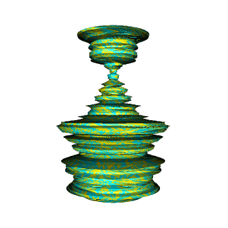
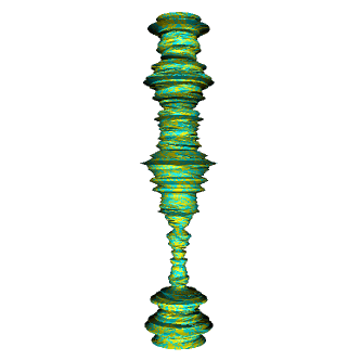
Figure 1: Typical configurations for $c\!=\!0$, with volumes $N\!=\!8100$ ($\tau\!=\!1$) and $N\!=\!9408$ ($\tau\!=\!3$). The spin configurations are those of a $\beta\!=\!0$ system.

From the point of view of the space-time geometry, the situation is similar for $c\!=\!1/2$ coupled to Lorentzian gravity. We illustrate this by two typical configurations, depicted in Fig. 2. Also in this case we have checked that the distribution $SV_{N}(l)$ is independent of the relative temporal extension $\tau$ of space-time.

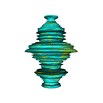
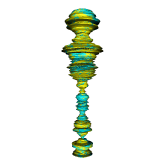
Figure 2: Typical configurations for $c\!=\!1/2$, with volumes $N\!=\!8100$ ($\tau\!=\!1$) and $N\!=\!9408$ ($\tau\!=\!3$).

3.2 Properties of the quantum geometry for $c=4$

3.2.1 The length distribution $SV_{N}(l)$ and the dimension of proper time

In the same manner as discussed above, we can extract some large-scale characteristics of the quantum geometry of the $c\!=\!4$ system coupled to Lorentzian gravity by studying the scaling properties of the distribution $SV_{N}(l)$ of one-dimensional spatial slices of volume $l$. It turns out that for $c\!=\!4$ one has to simulate systems with $\tau\geq 3$ to observe a clear scaling behaviour. As illustrated by Fig. 3,

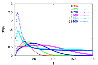
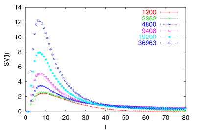
Figure 3: The appearance of spatial slices of very short length for $c\!=\!4$, and for $\tau\!=\!1$ (left) and $\tau\!=\!3$ (right).

the system exhibits a tendency for developing a large number of very short spatial slices, with length of the order of the cut-off. The length distribution $SV_{N}(l)$ has a peak at small $l$, whose height increases with $N$, but whose position has a very weak dependence on the system size. Since the volume is kept fixed, there are strong finite-size effects which artificially prohibit the system from forming such a peak whenever $N$ and $\tau$ are simultaneously small. This is obvious from the data taken for the $\tau\!=\!1$ system (Fig. 3). In that case the peak appears clearly only for a system with more than $8100$ vertices. Such finite-size effects are absent for the $\tau\!=\!3$ system.

These properties are well illustrated by Figs. 4 and 5, which show some typical geometries at $c\!=\!4$. They should be compared to our previous Figs. 1 and 2 for $c\leq 1/2$.

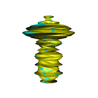
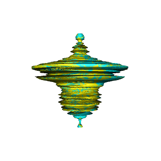
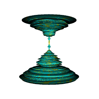
Figure 4: Typical configurations for $c\!=\!4$, $\tau\!=\!1$ and volumes $N\!=\!1024,8100$ and $32400$.

Fig. 4 contains space-time configurations at $\tau\!=\!1$, for three different volumes $N$. Their tendency to separate into two distinct regions increases with $N$ (remember that the time direction has been chosen periodic). This is a typical finite-$N$ behaviour associated with a phase transition, in this case, of the geometry. Likewise, for increasing $\tau$ (and constant volume) it becomes easier to form long and thin “necks”, along which the spatial volumes $l$ stay close to the cut-off size (see Fig. 5). Note in particular the space-time history with the largest volume ($N\!=\!36963$), where the separation of space-time into two different phases is very pronounced, underscoring at the same time the effect of increasing $N$. This figure also illustrates the fact that in the limit as $N\to\infty$, the neck region will carry a vanishing space-time volume.

It happens only rarely that the extended region shows a tendency to break up into smaller parts. Generally speaking, the fluctuations in its shape constitute the slowest modes of the simulation. Occasionally we observe a (much) smaller extended region splitting off from the main one. However, our statistics was insufficient to establish whether for large $\tau$ there is an underlying pattern governing the size and frequency of these events. For our present purposes, this effect can be safely ignored, since the number and size of such secondary space-time regions was small.

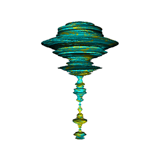
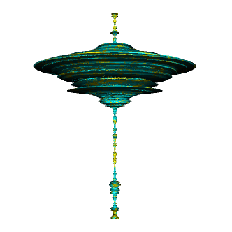
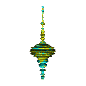
Figure 5: Typical configurations for $c\!=\!4$, with volumes $N\!=\!8192$ ($\tau\!=\!2$), $N\!=\!36963$ ($\tau\!=\!3$) and $N\!=\!8464$ ($\tau\!=\!4$).

Let us now quantify the scenario just outlined by a study of the scaling properties of $SV_{N}(l)$. As expected, the length distributions $SV_{N}(l)$ show no sign of scaling for small $l$. For large $l$, however, a scaling relation of type (3) is well satisfied, as illustrated by the plots in Fig. 6.

$\tau$=1	$\tau$=2	$\tau$=3	$\tau$=4
1.70(3)	1.65(5)	1.54(3)	1.50(3)

Table 2: The optimal values of the exponent $\delta_{h}$ for best scaling of $SV(l)$ fitting (3).

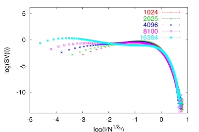
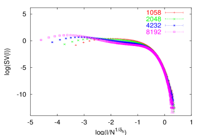
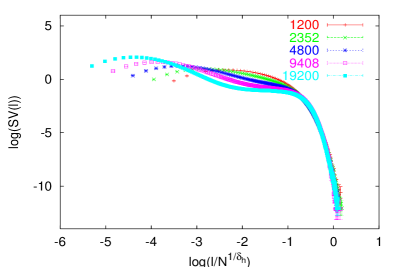
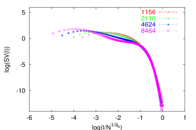
Figure 6: The distributions $SV(l)$ for the $c\!=\!4$, $\tau\!=\!1,2,3$ and $4$ systems.

The optimal values for $\delta_{h}$ are contained in Table 1. There is a clear tendency for $\delta_{h}\rightarrow 3/2$ as $\tau$ becomes large. From Fig. 6 we can read off at which value of the parameter $x=l/N_{T}^{\delta_{h}}$ the scaling sets in. This happens for $x\geq c$, where $c\approx 0.5$, or (setting $\delta_{h}\!=\!3/2$) for lengths

$$l\geq c\,N_{T}^{2/3}.$$ (8)

As mentioned above, the neck region does not contribute significantly to the volume for large $N$. We have measured that the volume $V_{ext}$ of the extended phase (now defined as the scaling region of $SV(l)$) is asymptotically proportional to the total volume $V$($\equiv N_{T}$) of the surface. Let $t_{ext}$ denote the temporal extension of this extended region and $l_{ext}$ the typical length of a spatial slice in that region (such that $t_{ext}\cdot l_{ext}=V_{ext}\propto N$). If we assume for the sake of definiteness that indeed $\delta_{h}\!=\!3/2$, it follows from (5) and (4) that

$${\rm dim}\,V_{ext} = \frac{3}{2}\,{\rm dim}\,l_{ext}.$$ (9)

From this we immediately deduce the relations

$${\rm dim}\,l_{ext} = 2\,{\rm dim}\,t_{ext},$$ (10)

$${\rm dim}\,V = 3\,{\rm dim}\,t_{ext},\,$$ (11)

and that the cosmological Hausdorff dimension is given by $d_{H}\!=\!3$.

Our main conclusion is that the coupling of 8 Ising models to Lorentzian gravity produces a phase transition in which some universal properties of the geometry are changed. At large distances, proper time and spatial length develop anomalous dimensions relative to each other and to the space-time volume, as expressed by eqs. (10) and (11).

3.2.2 The shell volume $n_{N}(r)$ and the short-distance dimension $d_{h}$

Next we discuss the measurement of the one-dimensional volumes $n_{N}(r)$ of spherical shells at distance $r$. It turns out that for $c\!=\!4$ Lorentzian gravity plus matter, these functions do not exhibit the universal scaling properties found elsewhere in models of two-dimensional gravity [5, 6, 8]. (That a universal behaviour at all length scales is unlikely is already illustrated by the separation of typical configurations into a thin and an extended region apparent in Fig. 5.) As discussed at the beginning of this section, this is no reason for concern; it simply reflects the fact that the underlying quantum geometry is more complex. We will identify several well-defined scaling regions and encounter the more general situation where the short-distance and the cosmological Hausdorff dimensions are different.

As can be seen in Fig. 7, the short-distance behaviour of $n_{N}(r)$ is independent of $N$ and can be fitted nicely to $n_{N}(r)\sim r^{d_{h}-1}$, with $d_{h}\approx 2$ (which coincides with the value found for $c\!=\!1/2$ and also happens to be the “canonical” dimension expected from classical considerations). The best fit gives $d_{h}=2.1(2)$.

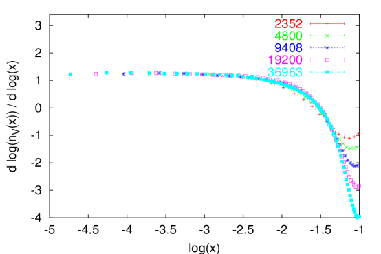
Figure 7: Small-distance scaling of the correlation function $n_{N}(r)$ for the $c\!=\!4$ system.

Going out to length scales of the order $r\sim N^{1/3}$, we see a different scaling behaviour. Here (6) is valid with a cosmological Hausdorff dimension $d_{H}\!=\!3$, in accordance with the value extracted from the measurements of the length distribution $SV_{N}(l)$. Finite-size scaling in this region, computed from the scaling of the peaks of $n_{N}(r)$ (Fig. 8), yields $d_{H}=3.07(9)$.

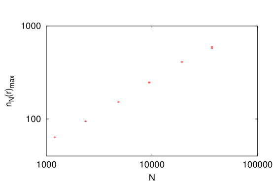
Figure 8: Scaling of the peaks of the correlation function $n_{N}(r)$ for the $c\!=\!4$ system.

Finally, at very large $r$ near the tail of the distribution, we found that the value of $n_{N}(r)$ is almost independent of $N$, indicating a dominance of configurations with $d_{H}\!=\!1$. Recalling the typical shape of configurations at $c\!=\!4$ (Fig. 5), this suggests the following interpretation. Each measurement of $n_{N}(r)$ involves the choice of a reference point, from which the geodesic distances $r$ are measured. Since almost no space-time volume is contained in the thin necks, the randomly chosen reference point will typically be located somewhere in the extended region. However, moving outwards from such a bulk point in spherical shells will for large $r$ eventually bring us back to the neck region, which in the large-$N$ limit has a length proportional to $\sqrt{N}$ (simply because $N\propto t^{2}$). Once the spherical shells have reached the neck region, the volume function $n_{N}(r)$ will just measure a one-dimensional structure.

3.3 Matter behaviour in the extended phase

We have seen above how a Lorentzian geometry separates into two distinct regions under the coupling to 8 Ising models. Since the thin, stalk-like region is effectively one-dimensional, a non-trivial matter behaviour can be expected only in the remaining, spatially extended space-time region. The computation of the matter exponents in this phase is subtle and requires some care. At the critical matter coupling $\beta_{c}$ we have measured the same set of observables as in our previous simulations [3]. Together with their expected finite-size scaling behaviour they are

$$\chi=N(\left\langle m^{2}\right\rangle-\left\langle|m|\right\rangle^{2})\sim N^{\gamma/\nu d_{H}}~{}~{}~{}~{}~{}~{}~{}~{}~{}~{}~{}~{}{\rm(susceptibility)}$$ (12)

$$D_{\ln|m|}=N\Big{(}\left\langle e\right\rangle-\frac{\left\langle e|m|\right\rangle}{\left\langle|m|\right\rangle}\Big{)}\sim N^{1/\nu d_{H}}~{}~{}~{}~{}~{}~{}(D_{\ln|m|}\equiv\frac{d\ln|m|}{d\beta})$$ (13)

$$D_{\ln m^{2}}=N\Big{(}\left\langle e\right\rangle-\frac{\left\langle em^{2}\right\rangle}{\left\langle m^{2}\right\rangle}\Big{)}\sim N^{1/\nu d_{H}}~{}~{}~{}~{}~{}(D_{\ln m^{2}}\equiv\frac{d\ln m^{2}}{d\beta}),$$ (14)

where $\gamma$ and $\nu$ are the critical exponents of the susceptibility and of the divergent spin-spin correlation length.

Initially we checked that for the case of a single Ising model, extending the geometries in the temporal direction (i.e. taking $\tau>1$) does not affect the Onsager exponents found in [3]. The results are tabulated in Table 3, and do not differ significantly from our previous results.

Observable	Exponent
$\chi$	$\frac{\gamma}{\nu d_{H}}$	0.84(1)
$D_{\ln|m|}$	$\frac{1}{\nu d_{H}}$	0.552(5)
$D_{\ln m^{2}}$	$\frac{1}{\nu d_{H}}$	0.550(4)

Table 3: Matter exponents for the $c\!=\!1/2$, $\tau\!=\!3$ model.

If one repeats this analysis naïvely for $c\!=\!4$, without taking into account geometric properties, no consistent scaling behaviour is found. For example, we find Onsager exponents for $\tau\!=\!1$, but these change when $\tau$ is increased. Although the spins in the “thin” phase cannot be critical, and contribute little to the space-time volume, the “transition” region, where the spatial length $l$ changes from cut-off length to $l$’s satisfying (8), apparently spoils the measurements, and there are considerable finite-size effects. The situation does not improve when the volume $V_{ext}$ is used instead of the total volume in the finite-size scaling.

It seems that the only way to study the critical matter behaviour for the case of eight Ising models is to isolate explicitly the contributions from the spins on the extended part of the Lorentzian geometry. For this we adopt the following procedure: for each configuration we measure the energy $E$ and magnetization $M$ on all vertices belonging to spatial slices whose length is greater than a cut-off $l_{0}(N)=c_{\tau}N^{1/\delta_{h}}$, and on all links contained in such slices or connecting two of them. The constants $c_{\tau}$ and $\delta_{h}$ are determined from the scaling regions of the length distributions $SV_{N}(l)$, with $c_{\tau}\approx 0.5$, as discussed in connection with eq. (8). Denote the numbers of such vertices and links by $N^{\prime}$ and $N_{L}^{\prime}$. We then compute the averages $e=E/N_{L}^{\prime}$ and $m=M/N^{\prime}$, and measure the expectation values $\left\langle N^{\prime}\right\rangle$ and $\left\langle N_{L}^{\prime}\right\rangle$.

Looking at the Monte Carlo time histories, we observe that whenever $N^{\prime}\neq 0$, $e$ and $m$ fluctuate stably around their mean values (even when the vertex number $N^{\prime}$ is close to $0$), whereas $E$ and $M$ vary slowly but considerably together with $N^{\prime}$. We can thus safely ignore the (relatively few) configurations with $N^{\prime}\!=\!0$. We have also computed the volume $V^{\prime}\equiv V_{ext}$ contributing to the scaling region of $SV(l)$ and performed finite-size scaling of the observables computed from the modified energy and magnetization averages $e$ and $m$. The results of this final analysis are summarized in Table 4. We have used a variety of different definitions of the system size, to demonstrate that the critical matter exponents extracted from finite-size scaling do not depend on them. We conclude that the critical matter behaviour of our model of eight Ising spins, on the part of space-time that possesses a non-trivial spatial extension, is governed by the Onsager exponents, and therefore lies in the same universality class as the model containing only a single copy of Ising spins.

Observable	Exponent	Onsager Value	$V^{\prime}$-scaling	$\left\langle N^{\prime}\right\rangle$-scaling	$\left\langle N_{L}^{\prime}\right\rangle$-scaling
$\chi$	$\frac{\gamma}{\nu d_{H}}$	0.875	0.85(1)	0.86(1)	0.85(1)
$D_{\ln|m|}$	$\frac{1}{\nu d_{H}}$	0.5	0.520(5)	0.520(2)	0.48(1)
$D_{\ln m^{2}}$	$\frac{1}{\nu d_{H}}$	0.5	0.511(5)	0.512(4)	0.48(1)

Table 4: Critical matter exponents for the $c\!=\!4$, $\tau\!=\!3$ model. We compare scalings with respect to different definitions of system size.

4 Discussion

In order to provide an interpretation for some of our results on 2d Lorentzian gravity coupled to multiple Ising spins, we first need to recall some characteristic geometric features of 2d Euclidean gravity. Consider the one-dimensional spherical “shell” consisting of all points separated from a given reference point by a geodesic distance $r$. This curve will in general be multiply connected. Let $\rho(l,r)$ denote the number of connected shell components of length $l$ at distance $r$. It is a remarkable and universal result in 2d Euclidean quantum gravity that $r$ and $l$ have a relative anomalous scaling of the form

$$l\propto r^{2}.$$ (15)

For pure 2d Euclidean quantum gravity this was first proved analytically in [10], where in the limit of infinite space-time volume $\rho$ was found to be

$$\rho(l,r)\propto\frac{1}{r^{2}}\left(c_{1}z^{-5/2}+c_{2}z^{-1/2}+c_{3}z^{1/2}\right)\mbox{e}^{-z},~{}~{}~{}z=l/r^{2}.$$ (16)

It was later checked numerically [8, 11] for various values $c<1$ of the central charge that in the infinite-volume limit the length distribution $r^{2}\rho(l,r)$ is only a function of the variable $z\!=\!l/r^{2}$. In addition, for $z>1$ the functional dependence on $c$ turns out to be rather weak. For a finite space-time volume $N$, it was found that $r^{2}\rho(l,r)$ can be approximated well by

$$r^{2}\rho(l,r)\propto f(z,l/N^{2/d_{H}}).$$ (17)

We can use this relation to calculate the expectation values of integer powers of the length $l$,

$$\left\langle l^{n}\right\rangle_{r,N}\equiv\sum_{l}l^{n}\rho(l,r)\buildrel N\;{\rm large}\over{\longrightarrow}N^{2n/d_{H}}F_{n}(r/N^{1/d_{H}}),~{}~{}~{}~{}n>1,$$ (18)

where the functions $F_{n}$ behave like [8]

$$F_{n}(x)\sim x^{2n}~{}~{}~{}{\rm for}~{}~{}~{}x<1.$$ (19)

For small $r\ll N^{1/d_{H}}$ we thus obtain

$$\left\langle l^{n}\right\rangle_{r,N}\sim r^{2n}~{}~{}~{}{\rm for}~{}~{}~{}n>1,$$ (20)

which is in accordance with relation (15), whereas for “cosmological” distances $r\sim N^{1/d_{H}}$ one finds

$$\left\langle l^{n}\right\rangle_{r,N}\sim N^{2n/d_{H}}~{}~{}~{}~{}{\rm for}~{}~{}~{}n>1.$$ (21)

It should be emphasized again that eqs. (19) and (20) seem to be universally true for 2d Euclidean quantum gravity theories with $c<1$ and require no cut-off in the continuum limit. To our knowledge they are the only non-trivial relations in 2d Euclidean quantum gravity independent of the central charge $c$.

For Lorentzian gravity coupled to a $c\!=\!4$ conformal field theory we saw above that the geometry had undergone a phase transition compared to $c\!=\!0$ and $c\!=\!1/2$. In those cases, a continuum limit could only be obtained if time and space had identical scaling dimensions, dim$\,l$ = dim$\,t$. Under the natural identification of Lorentzian proper time $t$ with the geodesic distance $r$ of the Euclidean formulae, this should be contrasted with dim$\,l$ = 2 dim$\,r$, which follows immediately from relation (15). The analogue of relation (21) for Lorentzian gravity with $c\!=\!0,1/2$ is given by

$$\left\langle l^{n}\right\rangle_{t,N}=N^{n/d_{H}},~{}~{}~{}~{}d_{H}=2,\hskip 28.45274ptn>0.$$ (22)

More precisely, eq. (22) can be computed exactly for $c\!=\!0$ and is deduced for $c\!=\!1/2$ by numerical comparison of the length distributions. However, the scaling relation we observed for $c\!=\!4$ was not (22), but (21) (for $n>0$)! The surprising conclusion is that with increasing central charge $c$ the geometry undergoes a transition from a state characterized by (22), to one satisfying (21), which is a generic property of Euclidean quantum gravity with $c<1$.

What causes this transition as more and more matter is added to the model? As discussed in [12, 13], matter has a tendency to “squeeze off” parts of space-time. In 2d Euclidean quantum gravity this pinching can take place anywhere and results in an ever-increasing number of baby universes. Eventually, for $c>1$, the fractal geometry degenerates into branched polymers, which can simply be viewed as a conglomerate of baby universes of the size of the cut-off.

In the Lorentzian case by construction no baby universes can be formed. The only possible way for matter to squeeze the geometry is to pinch constant-time slices to their minimal allowed spatial length $l\!=\!1$. This effect is very obvious in the Monte Carlo simulations and becomes more pronounced as the central charge is increased. In going to $c\!=\!4$ the influence of the matter has become so strong that a genuine phase transition has taken place. Only $t^{2/3}$ of the $t$ spatial slices (which typically occur together in a single extended region) have an extension beyond the cut-off scale. On the other hand their average spatial extension behaves like $t^{4/3}$. The remaining spatial slices have been pinched to the cut-off scale. On the fraction of slices with a macroscopic extension, one can then define a scaling limit, which at large distances is characterized by a Hausdorff dimension $d_{H}\!=\!3$. Likewise the relative dimensions of space and time are changed from their naïve canonical values dim$\,l$ = dim$\,r$, derived from (22), to dim$\;l$ =2 dim$\;r$, dictated by (21).

From our experience with Euclidean quantum gravity, this behaviour may seem unexpected. In that case, a large influence of the matter on the geometry is always accompanied by a large back reaction of the geometry on the matter, in the sense that the critical matter and gravity exponents always change simultaneously. (An exception to this is the relation (21), which is valid for all $c<1$ and therefore contains no information about the conformal field theory and its coupling to geometry.) The Lorentzian gravity model behaves differently: the matter strongly affects the geometry (changing bulk properties like the Hausdorff dimension and the relative scaling between time and spatial directions), but these apparently drastic changes are still not sufficient to alter any of the universal matter properties. Even when 8 Ising models are coupled to Lorentzian gravity, the critical matter exponents still retain their Onsager values.

This situation provides further support for the viewpoint advanced in our previous work [1, 3] that the critical gravity and matter behaviour of the Euclidean models is entirely determined by the presence of baby universes. In the light of our new results, the argument may be put as follows. So far it has been unclear whether the change in the critical exponents of conformal field theories when coupled to Euclidean quantum gravity was due to the strong back reaction of the geometry on the matter or to the baby universes that were present a priori. Lorentzian gravity with 8 Ising spins provides an example where undeniably the interaction of the matter and gravity sectors is strong. Nevertheless the critical Ising exponents remain unchanged. This strongly suggests that in the Euclidean case it is really the baby universes which are responsible for the observed changes in the universal properties of the matter.

While we have not undertaken a systematic search for the exact value of $c$ where the phase transition in geometry takes place, it is tempting to conjecture that it occurs at $c_{\it crit}\!=\!1$. Independent of the exact value of $c_{\it crit}$, we have identified a weak analogue of the $c\!=\!1$ barrier also in Lorentzian gravity. From the point of view of matter, nothing dramatic happens when the barrier is crossed. However, the behaviour of the quantum geometry undergoes a qualitative change and even shares some features with the non-singular part of the quantum geometries described by 2d Euclidean gravity coupled to matter with $c<1$. This highlights the universal nature of the relation $l\propto r^{2}$ and motivates the search for a simple underlying explanation, which may have a status similar to that of $d_{H}\!=\!2$ for Brownian motions.

5 Outlook

In closing, let us step back to examine the potential larger implications of all we have learned so far about two-dimensional Lorentzian quantum gravity. Our original aim was to find a non-perturbative path-integral formulation for quantum gravity. Previous attempts in this direction had largely been confined to the sector of Euclidean space-time metrics. Since for general metrics there is no straightforward analogue of the Wick rotation, a path integral over Lorentzian geometries is likely to require a more radical modification (compared with the Euclidean theory) than a mere analytic continuation of the action.

We chose to make the path integral Lorentzian by requiring each individual space-time geometry contributing to the state sum to carry a causal structure associated with a Lorentzian geometry. In order to make the construction well defined, a regularization is necessary, and we used the method of dynamical triangulations (where geometric manifolds are represented as gluings of $d$-dimensional simplices), which had previously been employed successfully in a Euclidean context. An ideal testing ground for such a proposal is gravity in dimension $d\!=\!2$, whose Euclidean sector (“Liouville gravity”) has been studied extensively by a variety of methods. We performed the Lorentzian state sum exactly, over a set of dynamically triangulated 2-geometries satisfying a (discrete analogue) of causality, and taking a continuum limit.

Maybe surprisingly, the resulting continuum theory turned out to be a new, bona fide theory of 2d quantum gravity fundamentally different from (Euclidean) Liouville gravity. As already mentioned in the introduction, it describes an ensemble of strongly fluctuating geometries, with local curvature degrees of freedom. Nevertheless, the geometry is less fractal than its Euclidean counterpart, and therefore closer to our intuitive, classical notions of smooth geometry.

The existence of at least two different quantum gravities constructed by rigorous path-integral methods in 2d raises the question of “which one is the right theory?” There is no ultimate answer to this, since two-dimensional gravity (never mind its signature) does not describe any phenomena of the real world. Aficionados of Liouville gravity might object by saying that the Lorentzian version of quantum geometry was surely the less interesting, with not enough “happening” compared with the Euclidean case where, for example, the Hausdorff dimension $d_{H}$ changes with the matter content. However, even if this were the case, it would not disqualify Lorentzian gravity from being a good candidate for a quantum gravity theory, since we do not know what the geometry of “real” quantum gravity looks like at the Planck scale. So far there is little evidence to suggest non-smoothness of the space-time geometry up to the grand unified scale, which itself after all is only a few orders of magnitude removed from the Planck scale.

At any rate, our present investigation shows that also in two-dimensional Lorentzian gravity things “do happen”. There is a strong interaction if one couples a sufficient amount of matter to Lorentzian geometry, affecting the universal properties of the combined system. In fact, one can argue that the resulting structure of quantum geometry is richer than that of the corresponding Euclidean model with matter, since its fractal structure (measured by the Hausdorff dimension) acquires a scale-dependence. Moreover, the interaction in Lorentzian gravity is strong, but – unlike in Euclidean gravity – not too strong in the sense of leading to a complete degeneration of the carrier geometry.

In a similar vein, evidence is accumulating that the structure of Euclidean quantum gravity with and without matter is governed entirely by the presence of baby universes (branching configurations not present in the Lorentzian version because of their incompatibility with causality). There is nothing wrong with this: statistical mechanical models of Euclidean gravity provide examples of generally covariant systems which are highly interesting in their own right. What they might teach us about quantum gravity proper is much less clear, since related (and from a classical point of view highly degenerate) branched-polymer configurations and their associated fractal structure play a central role in Euclidean gravity in higher dimensions too. There they seem to affect the theory in an undesirable way, making it difficult to obtain an interesting continuum limit of the statistical models of Euclidean quantum gravity in dimension $d>2$.

There is then a conclusion to be drawn for our eventual goal, the quantization of the physical theory of gravity in four space-time dimensions, whose character we know to be Lorentzian. Judging from our experience in two dimensions, the Lorentzian and Euclidean theories (if they both exist and are unique) may not be as closely related as is sometimes hoped for, invoking the example of standard, non-generally covariant quantum field theory. Our research has highlighted the importance of imposing causality (and thereby suppressing spatial topology changes) in the path integral over geometries. It remains to be seen which effect an analogous prescription has for quantum gravity theories in higher dimensions.