UKQCD’s latest results for the static quark potential and light hadron spectrum with $O(a)$ improved dynamical fermions.

Abstract

We present UKQCD’s latest results for the static quark potential and light hadron spectrum obtained from matched simulations using two flavours of dynamical quarks. We report that using matched ensembles helps disentangle screening effects from discretisation errors in the static quark potential.

1 Introduction

Previous simulations at fixed $\beta$ with several values of $\kappa_{\rm sea}$, have shown a strong dependence on the lattice spacing as $\kappa_{\rm sea}$ is varied [1]. This complicates the chiral extrapolations and obscures comparisons with quenched simulations. UKQCD have proposed that simulations should be carried out at fixed lattice spacing, $a$, for different values of $\kappa_{\rm sea}$. In this way it is possible to study the effect of varying the sea quark mass at the same effective lattice volume.

The lattice spacing is fixed by tuning the bare parameters, $\beta$ and $\kappa_{\rm sea}$. This is achieved by comparing a lattice observable with the physical value. In our case the Sommer scale, $r_{0}$,  [2] has been used, where,

$$F(r_{0}/a)(r_{0}/a)^{2}=1.65,\qquad r_{0}=0.49{\rm fm}$$ (1)

and $F(r_{0}/a)$ is the force between a static quark anti-quark pair. The Sommer scale was selected as it can be determined with good statistical precision and is independent of the valence quarks, avoiding the need for extrapolations. The details of the matching technique can be found in [3].

2 Simulation parameters

The simulations are performed with two flavours of dynamical fermions. We use the standard Wilson gauge action together with the $O(a)$ improved Wilson fermion action. The clover coefficient used was determined non-perturbatively by the Alpha Collaboration.

All simulations were carried out on a $16^{3}\times 32$ lattice. The parameters for the matched ensembles are shown in Table 1. The last entry shows a simulation at the lightest $\kappa_{\rm sea}$ which is not matched.

Table 1: Simulation parameters

$\beta$	$c_{\rm sw}$	$\kappa_{\rm sea}$	$\kappa_{\rm val}$	Conf.
5.29	1.92	0.1340	0.1335, 0.1340,	101
			0.1345, 0.1350
5.26	1.95	0.1345	0.1335, 0.1340	101
			0.1345, 0.1350
5.2	2.02	0.1350	0.1335, 0.1340,	150
			0.1345, 0.1350
5.9	1.89	Quen.	0.1325, 0.1330	100
			0.1335
Lightest $\kappa_{\rm sea}$ simulation.
5.2	2.02	0.1355	0.1340, 0.1345,	102
			0.1350, 0.1355

Table 2 shows the results for the lattice spacing and $r_{0}/a$ which were obtained using the method described in [4]. This corresponds to an effective lattice volume of approximately 1.7 fm for the matched simulations.

Table 2: Lattice spacing and $r_{0}/a$. The statistical error is in parentheses and the second error is an estimate of the systematic errors.

$\beta$	$\kappa_{\rm sea}$	$r_{0}/a$	$a[\rm fm]$
5.9	Quen.	4.332(45)	0.1131(12)$\;\begin{array}[]{@{}l@{}}\makebox[5.0pt][c]{$+$}\makebox[10.85004pt][r]{33}\\[-0.83997pt] \makebox[5.0pt][c]{$-$}\makebox[10.85004pt][r]{120}\end{array}$
5.29	.1340	4.450(61)$\;\begin{array}[]{@{}l@{}}\makebox[5.0pt][c]{$+$}\makebox[10.85004pt][r]{29}\\[-0.83997pt] \makebox[5.0pt][c]{$-$}\makebox[10.85004pt][r]{61}\end{array}$	0.1101(15)$\;\begin{array}[]{@{}l@{}}\makebox[5.0pt][c]{$+$}\makebox[10.85004pt][r]{13}\\[-0.83997pt] \makebox[5.0pt][c]{$-$}\makebox[10.85004pt][r]{7}\end{array}$
5.26	.1345	4.581(59)$\;\begin{array}[]{@{}l@{}}\makebox[5.0pt][c]{$+$}\makebox[10.85004pt][r]{0}\\[-0.83997pt] \makebox[5.0pt][c]{$-$}\makebox[10.85004pt][r]{120}\end{array}$	0.1070(14)$\;\begin{array}[]{@{}l@{}}\makebox[5.0pt][c]{$+$}\makebox[10.85004pt][r]{30}\\[-0.83997pt] \makebox[5.0pt][c]{$-$}\makebox[10.85004pt][r]{0}\end{array}$
5.2	.1350	4.576(80)$\;\begin{array}[]{@{}l@{}}\makebox[5.0pt][c]{$+$}\makebox[10.85004pt][r]{14}\\[-0.83997pt] \makebox[5.0pt][c]{$-$}\makebox[10.85004pt][r]{130}\end{array}$	0.1071(19)$\;\begin{array}[]{@{}l@{}}\makebox[5.0pt][c]{$+$}\makebox[10.85004pt][r]{40}\\[-0.83997pt] \makebox[5.0pt][c]{$-$}\makebox[10.85004pt][r]{3}\end{array}$
5.2	.1355	4.914(82)$\;\begin{array}[]{@{}l@{}}\makebox[5.0pt][c]{$+$}\makebox[10.85004pt][r]{70}\\[-0.83997pt] \makebox[5.0pt][c]{$-$}\makebox[10.85004pt][r]{19}\end{array}$	0.0997(17)$\;\begin{array}[]{@{}l@{}}\makebox[5.0pt][c]{$+$}\makebox[10.85004pt][r]{40}\\[-0.83997pt] \makebox[5.0pt][c]{$-$}\makebox[10.85004pt][r]{14}\end{array}$

3 Static quark potential

The standard form for the static quark potential

$$V(r)=V_{0}+\sigma r-\frac{e}{r},$$ (2)

can be rescaled in terms of $r_{0}$ as

$$[V(r)-V(r_{0})]r_{0}=(1.65-e)\left(\frac{r}{r_{0}}-1\right)-e\left(\frac{r_{0}}{r}-1\right)$$ (3)

Figure 1 shows the results for the static quark potential compared with eqn. 3. We observe good agreement with the universal fit $\pi/12r+\sigma r$. With these results there is no indication of string breaking at large $r/r_{0}$. However the plot of the deviation from the model shows significant discretisation errors. At short distances where the fits have to take this into account, there is some evidence that the lighter quark data lie below the heavier quark data.

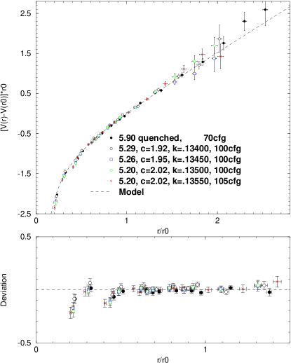
Figure 1: Rescaled static potential on matched ensembles compared with the string model.

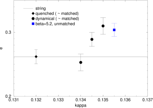
Figure 2: Fitted values of the parameter $e$ as a function of $\kappa_{\rm sea}$. The solid line is the Lüscher value $e=\frac{\pi}{12}$.

Parametric fits for the $1/r$ coefficient $e$, see Figure 2, show an increase for the dynamical data of $15\%\pm 4\%$. This is consistent with perturbation theory [5] which suggests an increase for $e$ of around $14\%$ for ${\rm N_{\rm f}}=2$.

Table 3: $m_{\rm PS}/m_{\rm V}$ ratios for dynamical data sets.

$\beta$	$\mbox{$\kappa_{\rm sea}$}=\mbox{$\kappa_{\rm val}$}$	$m_{\rm PS}/m_{\rm V}$
5.29	0.1340	0.830$\;\begin{array}[]{@{}l@{}}\makebox[5.0pt][c]{$+$}\makebox[10.85004pt][r]{8}\\[-0.83997pt] \makebox[5.0pt][c]{$-$}\makebox[10.85004pt][r]{6}\end{array}$
5.26	0.1345	0.785$\;\begin{array}[]{@{}l@{}}\makebox[5.0pt][c]{$+$}\makebox[10.85004pt][r]{9}\\[-0.83997pt] \makebox[5.0pt][c]{$-$}\makebox[10.85004pt][r]{9}\end{array}$
5.2	0.1350	0.693$\;\begin{array}[]{@{}l@{}}\makebox[5.0pt][c]{$+$}\makebox[10.85004pt][r]{11}\\[-0.83997pt] \makebox[5.0pt][c]{$-$}\makebox[10.85004pt][r]{13}\end{array}$
5.2	0.1355	0.584$\;\begin{array}[]{@{}l@{}}\makebox[5.0pt][c]{$+$}\makebox[10.85004pt][r]{25}\\[-0.83997pt] \makebox[5.0pt][c]{$-$}\makebox[10.85004pt][r]{16}\end{array}$

4 Light hadron spectrum

Hadron masses were obtained from correlated least-$\chi^{2}$ fits. The mesons have been fitted by a double cosh fit to local and fuzzed correlators simultaneously. Baryons are fitted by a single exponential fit to fuzzed correlators only. The ratio of the pseudoscalar to vector masses is shown in Table 3 for $\mbox{$\kappa_{\rm sea}$}=\mbox{$\kappa_{\rm val}$}$. One way to look for dynamical effects in the spectrum is to compare the pseudoscalar and vector meson masses as $\kappa_{\rm sea}$ is varied. Figure 3 shows a plot of $m_{\rm V}$ against $m^{2}_{\rm PS}$ for all data sets. Since $\beta$ is different for each data set, the results for the meson masses are shown in units of $r_{0}$. Points corresponding to $\mbox{$\kappa_{\rm sea}$}=\mbox{$\kappa_{\rm val}$}$ are indicated by arrows. This plot shows that there is a trend towards the experimental points as $\kappa_{\rm sea}$ becomes lighter.

Figure 3: Vector mass against pseudoscalar mass squared in units of $r_{0}$. The arrows indicate those points where $\mbox{$\kappa_{\rm sea}$}=\mbox{$\kappa_{\rm val}$}$.

Preliminary analysis of the spectrum has been conducted in the partially quenched scheme where the partially quenched quark mass is defined as

$$m_{q}^{\rm PQ}=\frac{1}{2}\left(\frac{1}{\mbox{$\kappa_{\rm val}$}}-\frac{1}{\kappa_{\rm crit}}\right)$$ (4)

Here $\kappa_{\rm crit}$ has been determined from an extrapolation in the improved valence quark mass for each data set, $am_{\rm PS}^{2}\propto\tilde{m}_{q}(\mbox{$\kappa_{\rm val}$})$, using $b_{\rm m}$ from perturbation theory.

The pseudoscalar extrapolation as a function of $m_{q}^{\rm PQ}$ is shown for all data sets in Figure 4. A straight line has been fitted to the matched data sets, including the quenched simulation, using an uncorrelated fit. Data points from the lightest $\kappa_{\rm sea}$ simulation have been included in the plot. These points clearly have a different slope from the matched data sets.

Figure 4: Pseudoscalar extrapolation as a function of the partially quenched quark mass in lattice units.

5 Conclusions

We have seen some evidence of screening in the static quark potential for dynamical ${\rm N_{\rm f}}=2$ simulations. Using data sets which have been matched to have the same effective lattice volume helps to disentangle the screening effects from the discretisation errors in the potential. Extrapolations of the pseudoscalar mass as a function of the partially quenched quark mass, show that the slope is consistent for the matched ensembles. Further analysis of this type of extrapolation is in progress.

References

• [1] UKQCD, Phys.Rev.D ย 60 (1999) 034507
• [2] R.ย Sommer, Nucl.Phys.B ย 411 (1994) 839
• [3] A.C.ย Irving et al., Phys.Rev.D ย 58 (1998) 114504
• [4] R.G.ย Edwards et al., Nucl.Phys.B ย 517 (1998) 337
• [5] El. Khadra et al., Phys.Rev.Lett ย 69 (1992) 729