Truncated Overlap Fermions

Abstract

In this talk I propose a new computational scheme with overlap fermions and a fast algorithm to invert the corresponding Dirac operator.

1 INTRODUCTION

After many years of research in lattice QCD, it was possible to formulate QCD with chiral fermions on the lattice [1, 2, 3, 4].

The basic idea is an expanded flavor space which may be seen as an extra dimension with left and right handed fermions defined in the two opposite boundaries or walls.

Let $N$ be the size of the extra dimension, $D_{W}$ the Wilson-Dirac operator, and $m$ the bare fermion mass. Then, the theory with Domain Wall Fermions is defined by the action [1, 2]:

$$\begin{array}[]{l}S_{DW}:=\bar{\Psi}{\cal{M}}\Psi=\sum_{i=1}^{N}\bar{\psi}_{i}[(D^{||}-1)\psi_{i}\\ +P_{+}\psi_{i+1}+P_{-}\psi_{i-1}],\\ P_{+}(\psi_{N+1}+m\psi_{1})=0,~{}~{}P_{-}(\psi_{0}+m\psi_{N})=0\end{array}$$ (1)

where $\cal{M}$ is the five-dimensional fermion matrix of the regularized theory and $D^{||}=M-D_{W}$ with $M\in(0,2)$ being a mass parameter.

In this talk I define a theory with Truncated Overlap Fermions in complete analogy with the Domain Wall Fermions by substituting

$$\begin{array}[]{l}P_{+}\psi_{i+1}\rightarrow(D^{||}+1)P_{+}\psi_{i+1}\\ P_{-}\psi_{i-1}\rightarrow(D^{||}+1)P_{-}\psi_{i-1}\end{array}$$ (2)

while the boundary conditions remain the same as before.

Both theories can be compactified in the walls of the extra fifth dimension as low energy effective theories (see below) with the chiral Dirac operator $D$ satisfying the Ginsparg-Wilson relation [5]:

$$\gamma_{5}D^{-1}+D^{-1}\gamma_{5}=2a\gamma_{5}R,$$ (3)

where $a$ is the lattice spacing and $R$ is a local operator trivial in the Dirac space (see below for $R$-locality tests). From now on I set $a=1$.

I defined Truncated Overlap Fermions such that in the large $N$ limit one obtains Overlap Fermions [3] with the Dirac operator given by [6]:

$$D_{OV}=\frac{1+m}{2}-\frac{1-m}{2}\gamma_{5}\mbox{sgn}(H)$$ (4)

where $H=\gamma_{5}D^{||}$.

Until now computations with chiral fermions and standard algorithms have been very expensive. The extra fermion flavors introduce a large overhead. One multiplication with the fermion matrix costs ${\cal{O}}(n)$ $D_{W}$-multiplications with $n\sim N$ for Domain Wall Fermions and much larger for the overlap operator [7, 8, 9].

In this talk I propose a fast algorithm which makes these simulations an order of magnitude faster. The key observation is the lack of gauge connections along the fifth dimension.

2 TRUNCATED OVERLAP FERMIONS

I recall the action of the Truncated Overlap Fermions:

$$\begin{array}[]{l}S_{TOV}:=\bar{\psi}_{1}[(D^{||}-1)\psi_{1}\\ +(D^{||}+1)P_{+}\psi_{2}-m(D^{||}+1)P_{-}\psi_{N}]\\ +\sum_{i=2}^{N-1}\bar{\psi}_{i}[(D^{||}-1)\psi_{i}\\ +(D^{||}+1)P_{+}\psi_{i+1}+(D^{||}+1)P_{-}\psi_{i-1}]\\ +\bar{\psi}_{N}[(D^{||}-1)\psi_{N}\\ -m(D^{||}+1)P_{+}\psi_{1}+(D^{||}+1)P_{-}\psi_{N-1}]\end{array}$$ (5)

Let $P^{T}$ be the matrix representing the unitary transformation:

$$\begin{array}[]{l}\chi_{1}=P_{+}\psi_{1}+P_{-}\psi_{N},\\ \chi_{i}=P_{+}\psi_{i}+P_{-}\psi_{i-1},~{}~{}i=2,\ldots,N\end{array}$$ (6)

and $S$ the matrix representing the diagonal transformation: $\bar{\chi}_{i}=\bar{\psi}_{i}\gamma_{5}(H-1),~{}~{}i=1,\ldots,N$. Let also the transfer matrix along the fifth dimension be defined by: $T=\frac{1+H}{1-H}$.

In the new basis I obtain the following action:

$$\begin{array}[]{l}S_{TOV}=\bar{\chi}_{1}[(P_{+}-mP_{-})\chi_{1}-T\chi_{2}]\\ +\sum_{i=1}^{N-1}\bar{\chi}_{i}(\chi_{i}-T\chi_{i+1})\\ +\bar{\chi}_{N}[\chi_{N}-T(P_{-}-mP_{+})\chi_{1}]\end{array}$$ (7)

Integrating over the Grassmann fields I get:

$$\mbox{det}{\cal{M}}=\mbox{det}[(P_{+}-mP_{-})-T^{N}(P_{-}-mP_{+})]$$ (8)

where I ignore the Jacobian factor coming from the diagonal transformation.

If ${\cal{M}}_{1}$ is the same matrix as $\cal{M}$ but with the special choice $m=1$, I define the effective low energy theory with the Dirac operator given by the equations:

$$D=(P^{T}{\cal{M}}_{1}^{-1}{\cal{M}}P)_{1,1},~{}D^{-1}=(P^{T}{\cal{M}}^{-1}{\cal{M}}_{1}P)_{1,1}$$ (9)

where the subscript $1,1$ stands for the $(1,1)$ block of an $N$x$N$ partitioned matrix along the fifth dimension.

In terms of the transfer matrix the Dirac operator can be written as:

$$D=\frac{1+m}{2}+\frac{1-m}{2}\gamma_{5}\frac{1-T^{N}}{1+T^{N}}$$ (10)

I can repeat this derivation for the Domain Wall Fermions with the sole changes $\bar{\chi}_{i}=\bar{\psi}_{i}\gamma_{5}(HP_{+}-1),~{}~{}i=1,\ldots,N$ and $T=\frac{1}{1-HP_{+}}(1+HP_{-})$, the rest of the formulae remaining the same.

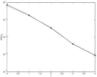
Figure 1: Norm of $D$ kernel in spin and color space with the distance $r$ from the origin for $N=4$ (circles) and $N=32$ (crosses).

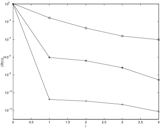
Figure 2: Norm of $R$ kernel in spin and color space with the distance $r$ from the origin for $N=4$ (circles), $N=32$ (crosses) and $N=64$ (pluses).

3 LOCALITY AND GINSPARG- WILSON RELATION TESTS

I test the Ginsparg-Wilson relation for the Truncated Overlap Fermions, so that they can be used like Domain Wall Fermions.

I computed the norm of $D$ and $R$ kernels in spin and color space with the distance $r=\sqrt{x_{\mu}x_{\mu}}$ from the origin on $4^{4}$ lattices at $\beta=6.0$. In Figs. 1 and 2 I show the maximum values at on-axis distances. Note that $x_{\mu},\mu=1,2,3,4$ is measured modulo lattice size in that direction.

Fig. 1 suggests exponential fall-off of $||D(r)||_{2}$, whereas Fig. 2 shows that $R$ approaches a Kronecker-Delta function as $N$ grows.

4 A FAST INVERSION ALGORITHM

I use Truncated Overlap fermions to define the following

ALGORITHM1 (Generic) for solving the system $D_{OV}x=b$:

$$\begin{array}[]{l}\mbox{Given}~{}N,~{}x_{0},~{}r_{0}(=b),~{}tol,~{}tol_{1},~{}\mbox{set}~{}tol_{0}=1\\ \mbox{and iterate:}\\ for~{}i=1,\ldots\\ ~{}~{}~{}~{}tol_{0}=tol_{0}tol_{1}\\ ~{}~{}~{}~{}{\bf\mbox{Solve}~{}Dy=r_{i-1}~{}\mbox{within}~{}tol_{0}}\\ ~{}~{}~{}~{}x_{i}=x_{i-1}+y\\ ~{}~{}~{}~{}{\bf r_{i}=b-D_{OV}x_{i}}\\ ~{}~{}~{}~{}if||r_{i}||_{2}<tol,~{}end~{}for\\ \end{array}$$ (11)

where by $o$ is denoted a vector with zero entries and $tol_{1},tol$ are tolerances. $tol_{1}$ is typically orders of magnitude larger than $tol$ such that the work per $D_{OV}$ inversion is minimized.

Remark 1. Bold face equations represent the smaller system soultion and the correction of the right-hand side. The straightforward application of the $ALGORITHM1$ gives a two-level algorithm. By calling it again in solving the smaller system and iterating, one gets a multi-level algorithm.

In Fig. 3 I compare the norm of the residual $r_{i}=b-D_{OV}x_{i}$ of the Conjugate Residual (CR) algorithm (which is optimal since $D_{OV}$ is normal [10]) and $ALGORITHM1$. I gain about an order of magnitude (in average) on $30$ $4^{4}$-configurations at $\beta=6.0$ and $m=0.1$. For the coarse lattice I used $N=6$ with the Truncated Overlap Fermions and the Lanczos method to compute $D_{OV}$ [7].

Remark 2. Dynamical fermions can be implemented similarly. The corresponding Hybrid Monte Carlo (HMC) algorithm can be obtained by working with an approximate Hamiltonian in the coarse lattice and by a global correction on the fine lattice.

One may use also as a starting point Truncated Overlap Fermions: det$D=$det${\cal M}/$det${\cal M}_{1}$. This way, all known simulation algorithms for dynamical fermions apply.

5 CONCLUSIONS

I showed that Truncated Overlap Fermions may be used in two ways:

a) to implement Overlap Fermions in the same fashion as Domain Wall Fermions;

b) to construct a multi-level inversion algorithm for Overlap Fermions which saves an order of magnitude of computer time compared to the state of the art methods.

Further tests are needed to verify these results on larger lattices.

Recently, the possibility of a Multigrid algorithm along all dimensions is raised [11]. In this case a gauge fixing is needed.

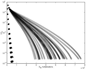
Figure 3: Norm of the residual error vs. the number of $D_{W}$ multiplications on 30 configurations. Circles stand for the straightforward inversion and stars for the new algorithm.

6 Acknowledgements

The author would like to thank John Ellis for the hospitality at CERN where these ideas initiated and for discussions on the chiral fermions.

I would like to thank Philippe de Forcrand for suggestions on how to improve the $ALGORITHM1$ which I will consider in the future.

The author thanks PSI where this work was done and SCSC Manno for the allocation of computer time on the NEC SX4.

References

- [1] D.B. Kaplan, Phys. Lett. B 228 (1992) 342.
- [2] Y. Shamir, Nucl. Phys. B 406 (1993) 90; V. Furman and Y. Shamir, Nucl. Phys. B (1995) 54.
- [3] R. Narayanan, H. Neuberger, Phys. Lett. B 302 (1993) 62, Nucl. Phys. B 443 (1995) 305.
- [4] P. Hasenfratz, V. Laliena and F. Niedermayer, Phys. Lett. B 427 (1998) 125.
- [5] P. H. Ginsparg and K. G. Wilson, Phys. Rev. D 25 (1982) 2649.
- [6] H. Neuberger, Phys. Lett. B 417 (1998) 141, Phys. Rev. D 57 (1998) 5417.
- [7] A. Boriçi, Phys. Lett. B 453 (1999) 46.
- [8] H. Neuberger, Phys. Rev. Lett. 81 (1998) 4060.
- [9] R. G. Edwards, U. M. Heller and R. Narayanan, FSU-SCRI-98-71, and hep-lat/9807017.
- [10] A. Boriçi, Krylov Subspace Methods in Lattice QCD, PhD Thesis, CSCS TR-96-27, ETH Zürich 1996.
- [11] L. Giusti, Ch. Hoelbling and C. Rebbi, hep-lat/9906004 and these proceedings.