Topology in CP^N-1 models: a critical comparison of different cooling techniques

Abstract

Various cooling methods, including a recently introduced one which smoothes out only quantum fluctuations larger than a given threshold, are applied to the study of topology in 2d CP^N-1 models. A critical comparison of their properties is performed.

Two-dimensional CP^N-1 models play an important role in quantum field theory because they share many properties with QCD. In particular, they possess instanton classical solutions and one can define topological charge and susceptibility in analogy with QCD. CP^N-1 models represent therefore a useful theoretical laboratory to investigate numerical methods to be eventually applied to study the topology in QCD. One of the most powerful tools for the study of the topological structure of the vacuum is the “cooling” method. It consists in measuring the topologically relevant quantities on the ensemble of lattice configurations obtained by replacing each equilibrium configuration by the one resulting after a sequence of local minimizations of the action.

The aim of this work is to get insight into a new cooling method first adopted in Ref. [1], by comparing it with the “standard” [2] and with its “controlled” version adopted by the Pisa group [3].

We chose the standard discretization for the action of the 2d CP^N-1 model:

$$S^{L}\!=\!-N\beta\sum_{n,\mu}\left(\bar{z}_{n+\mu}z_{n}\lambda_{n,\mu}\!+\!\bar{z}_{n}z_{n+\mu}\bar{\lambda}_{n,\mu}\!-\!2\right)$$ (1)

where $z_{n}$ is an $N-$component complex scalar field with $\bar{z}_{n}\cdot z_{n}=1$, $\lambda_{n,\mu}$ is a U(1) gauge field satisfying $\bar{\lambda}_{n,\mu}\lambda_{n,\mu}=1$ and $\beta=1/(Ng)$, with $g$ the lattice coupling. We used the standard action both in Monte Carlo simulations and in the cooling instead of any improved lattice action, since we wanted to test the cooling techniques in a situation where cutoff effects are large. The lattice topological charge density was defined as

$$q^{L}(x)\!=\!-{i\over 2\pi}\sum_{\mu\nu}\epsilon_{\mu\nu}{\rm Tr}\left[P(x)\Delta_{\mu}P(x)\Delta_{\nu}P(x)\right],$$ (2)

with

$$\Delta_{\mu}P(x) \equiv \frac{P(x{+}\mu)-P(x{-}\mu)}{2}~{},$$

$$P_{ij}(x) \equiv \bar{z}_{i}(x)z_{j}(x)\,,$$ (3)

giving for the lattice topological susceptibility

$$\chi^{L}\equiv\biggl{\langle}\sum_{x}q^{L}(x)q^{L}(0)\biggr{\rangle}={1\over L^{2}}\left<\left(Q^{L}\right)^{2}\right>\;,$$ (4)

where $Q^{L}\equiv\sum_{x}q^{L}(x)$ and $L$ is the lattice size. The cooling algorithm consists in assigning to each lattice variable $z_{n}$ and $\lambda_{n,\mu}$ a new value $z_{n}^{\mathrm{new}}$ and $\lambda_{n,\mu}^{\mathrm{new}}$ which locally minimizes the action, keeping all other variables fixed. In the “standard cooling” these replacements are unconstrained. We will call “new cooling” the one for which the replacements are done only if the angle $\alpha$ between the new and the old field variables, is larger than a given value $\delta$, and “Pisa cooling” the one for which the local minimization is performed with the constraint $\alpha\leq\delta_{\rm Pisa}$. Notice that between the “Pisa cooling” and the “new cooling” there is a substantial difference: while “Pisa cooling” acts first on the smoother fluctuations, the “new cooling” performs local minimizations only if these fluctuations are larger than a given threshold. Moreover the “new cooling” automatically stops when there are no more fluctuations beyond the threshold. It should be pointed out that any cooling procedure causes a partial loss of the topological content of the cooled configuration (namely “small instantons”). However this loss occurs at a fixed scale in lattice units and thus vanishes in the continuum limit, unless the instantons distribution is ultraviolet singular (as in the case of CP¹).

We considered first an “artificial” 1-instanton configuration discretized on the lattice. Although the three different cooling procedures act differently, since they start to deform the configuration in different regions, the curves for $Q^{L}$ and $S^{L}$ under the three coolings as a function of the instanton size $\rho$ fall on top of each other (see Fig. 1).

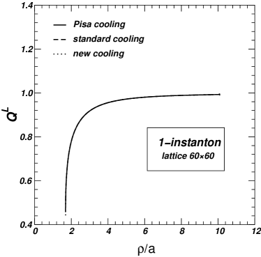
Figure 1: $Q^{L}$ vs $\rho/a$ under the three different cooling procedures. The instanton size is determined by $S^{L\;{\mathrm{max}}}=2/(\rho/a)^{2}$, ($a$ is the lattice spacing).The three curves fall exactly on top of each other.

We determined the topological susceptibility using the “new cooling” and compared the results with those from the “field theoretical method” [4]. In the field theoretical approach one has

$$\chi^{L}(\beta) = a^{2}Z(\beta)^{2}\chi^{\mathrm{cont}}+M(\beta)+O(a^{4})$$

$$M(\beta) = a^{2}\,A(\beta)\langle S(x)\rangle_{\mathrm{np}}+P(\beta)\langle I\rangle\;,$$ (5)

where $Z(\beta)$ is a finite multiplicative renormalization of the discretized topological charge density [5], while $M(\beta)$ is an additive renormalization containing mixing to operators of equal or lower dimension and same quantum numbers, namely the action density and the identity operator. On the lattice $\chi^{L}(\beta)$ is measured during the Monte-Carlo simulation, and $\chi^{\rm cont}$ is extracted by subtracting the renormalizations, which are computed non-perturbatively on the lattice by means of the “heating method” [6] ($Z$ and $P$ can be also computed perturbatively [7]). The “field theoretical method” can be improved by using a smeared topological charge density operator [8], built from the standard operator by replacing the fields $z$ and $\lambda_{\mu}$ with smeared fields $z^{\mathrm{smear}}$ and $\lambda_{\mu}^{\mathrm{smear}}$. In this way the renormalizations are strongly reduced and a much better accuracy is achieved for $\chi^{\rm cont}$.

We performed numerical simulations for $N=4$, $10$, $21$. The simulation algorithm is a mixture of 4 microcanonical updates and 1 over-heat bath. For each simulation we collected 100K configurations after 10K thermalization updating steps. We used several values of the $\delta$ parameter in the “new cooling” algorithm, while for the “Pisa cooling” we considered $\delta_{\mathrm{Pisa}}=0.2$. To set the scale we have taken the correlation length $\xi_{G}$ defined as the second moment of the correlation function $\langle\mbox{Tr}P(x)\,P(0)\rangle$. In Fig. 2 we show the behavior of $\chi^{L}$ on configurations cooled by the “new cooling” with different $\delta$’s, while in Fig. 3 we plot $\chi^{\rm cont}\xi_{G}^{2}$ for the values of $\delta$ which correspond to the peak region in $\chi^{L}$ in Fig. 2 and compare the results with the field theoretical determination (with and without smearing). There is consistency between the two determinations for all the considered values of $\delta$, which correspond to those for which the smoothing of the configuration is better.

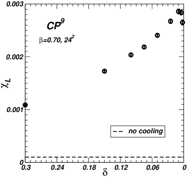
Figure 2: $\chi^{L}$ as a function of $\delta$ at $\beta=0.70$ on a $24^{2}$ lattice for CP⁹.

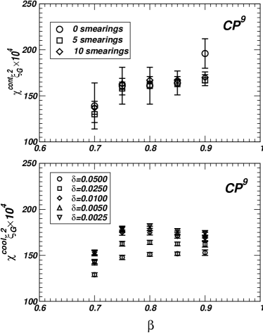
Figure 3: $\chi^{\rm cont}\xi_{G}^{2}$ for CP⁹ for several $\delta$ values ($L/\xi\simeq 10$ for all the points).

We have also calibrated the three cooling techniques (number of cooling steps for the standard and Pisa cooling versus $\delta$ for the new cooling) in order that the average energy on the ensemble cooled in the three different ways is the same. Then, comparing by eye several thermal configurations obtained after equivalent amounts of the three coolings, we have observed that the distributions and the shape of the instanton bumps is roughly the same. Also the values of $\chi^{\rm cont}\xi_{G}^{2}$ obtained after “equivalent” coolings are in agreement within the statistical errors. The only measurement where we could see a discrepancy is that of the “shell” correlation function of the topological charge density $\langle q_{L}(r)q_{L}(0)\rangle$ (see Fig. 4), which is slightly larger in the case of the new cooling method in the short distance region, with respect to the standard and Pisa coolings.

Our conclusion is that, except for the last observation which deserves further study, there is no appreciable difference between the three types of cooling we have investigated.

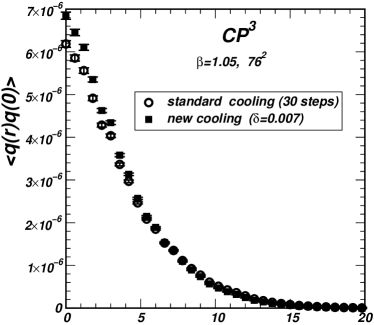
Figure 4: “Shell” correlation function of the lattice topological charge density ($r$ is the distance between two lattice sites).

References

- [1] M. García Pérez, O. Philipsen, I.O. Stamatescu, Nucl. Phys. B551 (1999) 293.
- [2] M. Teper, Phys. Lett. B171 (1986) 81 and 86.
- [3] M. Campostrini, A. Di Giacomo, H. Panagopoulos, E. Vicari, Nucl. Phys. B (Proc. Suppl.) 17 (1990) 634.
- [4] M. Campostrini, A. Di Giacomo, H. Panagopoulos, E. Vicari, Nucl. Phys. B329 (1990) 683.
- [5] M. Campostrini, A. Di Giacomo, H. Panagopoulos, Phys. Lett. B212 (1988) 206.
- [6] A. Di Giacomo, E. Vicari, Phys. Lett. B275 (1992) 429.
- [7] F. Farchioni, A. Papa, Phys. Lett. B306 (1993) 108.
- [8] C. Christou, A. Di Giacomo, H. Panagopoulos, E. Vicari, Phys. Rev. D53 (1996) 2619.