$U(1)$ Chiral Gauge Theory with Domain Wall Fermions and Gauge Fixing

Abstract

We investigate a U(1) lattice chiral gauge theory ($L\chi GT$) with the waveguide formulation of the domain wall fermions and with compact gauge fixing. In the reduced model limit, there seems to be no mirror chiral modes at the waveguide boundary.

1 Introduction

Gauge fixing is not necessary in Wilson lattice gauge theory. For gauge-non-invariant theories, if gauge fixing is not done with a target gauge-invariant theory in mind, however, there are nontrivial consequences, namely, the longitudinal gauge degrees of freedom (dof) couple to physical dof. The well-known example is the Smit-Swift proposal of $L\chi GT$. The obvious remedy is to gauge fix. The Roma proposal involving gauge fixing passed perturbative tests but does not address the problem of gauge fixing of compact gauge fields and the associated problem of lattice artifact Gribov copies. The formal problem is that for compact gauge-fixing a BRST-invariant partition function as well as (unnormalized) expectation values of BRST invariant operators vanish as a consequence of lattice Gribov copies. Shamir and Golterman [1] has proposed to keep the gauge-fixing part of the action BRST non-invariant and tune counterterms to recover BRST in the continuum. In their formalism, the continuum limit is to be taken from within the broken ferromagnetic (FM) phase approaching another broken phase which is called ferromagnetic directional (FMD) phase, with the mass of the gauge field vanishing at the FM-FMD transition. This was tried out in a U(1) Smit-Swift model [3] and so far all indications are that in the pure gauge sector, QED is recovered in the continuum limit and in the reduced model limit free chiral fermions in the appropriate chiral representation are obtained.

We want to extend this idea to other previous proposals of a $L\chi GT$ which supposedly failed due to above mentioned coupling of longitudinal gauge dof to physical dof. For this pupose we have chosen the waveguide formulation of the domain wall fermion where mirror chiral modes appeared at the waveguide boundary in addition to the chiral modes at the domain wall or antiwall to spoil the chiral nature of the theory [2].

2 Gauge-fixed Domain Wall Action

For Kaplan’s free domain wall fermions on a $4+1$-dimensional lattice of size $L^{4}L_{s}$ where $L_{s}$ is the 5th dimension, with periodic boundary conditions in the 5th or $s$-direction, there is always an anti-domain wall and the model possesses two zero modes of opposite chirality, one bound to the domain wall at $s=0$ and the other bound to the antiwall at $s=\frac{L_{s}}{2}$. With the domain wall mass $m(s)$ taken as

$$m(s)=\begin{array}[]{cl}-m_{0}&~{}~{}~{}~{}~{}0<s<\frac{L_{s}}{2}\\ 0&~{}~{}~{}~{}~{}s=0,\frac{L_{s}}{2}\\ m_{0}&~{}~{}~{}~{}~{}\frac{L_{s}}{2}<s<L_{s}\end{array}$$

the wall mode is lefthanded (LH), the antiwall mode is righthanded (RH). If $m_{0}L_{s}\gg 1$, these modes would have exponentially small overlap. These chiral modes exist for momenta $p$ below a critical momentum $p_{c}$, i.e. $|\hat{p}|<p_{c}$, where $\hat{p}^{2}=2\sum_{\mu}[1-cos(p_{\mu})]$ and $p_{c}^{2}=4-2m_{0}/r$.

Since the LH and RH modes of the fermion are separated in $s$ space, one can attempt to couple these two in different ways to a gauge field. A 4-dimensional gauge field which is same for all $s$-slices can be coupled to fermions only for a restricted number of $s$-slices around the anti-domain wall [2] with a view to coupling only to the RH mode at the antiwall. The gauge field is thus confined within a waveguide, $WG=(s:s_{0}<s\leq s_{1})$. Our choice of $s_{0}$ and $s_{1}$ is such that the anti-domain wall is located at the center of the $WG$, and at the same time far enough from the domain or anti-domain wall that the zeromodes are exponentially small at the $WG$ boundary [2]: $s_{0}=\frac{L_{s}+2}{4}-1$, $s_{1}=\frac{3L_{s}+2}{4}-1$. With this choice $L_{s}-2$ has to be a multiple of four. The global symmetry of the model and the gauge transformations on the fermion field in and outside $WG$ remain exactly the same as in ref. [2]. Obviously, the hopping terms from $s_{0}$ to $s_{0}+1$ and that from $s_{1}$ to $s_{1}+1$ would break the local gauge invariance of the action. This is taken care of by gauge transforming the action and thereby picking up the pure gauge dof or a radially frozen scalar field $\phi$ (Stückelberg field) at the $WG$ boundary. So the gauge invariant $WG$ action now becomes, retaining only the $s$ index, taking the Wilson $r=1$ and lattice constant $a=1$,

$$S_{F}\!\!\!\!\! = \!\!\!\!\!\!\!\sum_{s\in WG}\overline{\psi}^{s}\left(D\!\!\!\!/~{}(U)-W(U)+m(s)\right)\psi^{s}$$ (1)

$$+ \!\!\!\!\!\sum_{s\not\in WG}\overline{\psi}^{s}\left(\partial\!\!\!/-w+m(s)\right)\psi^{s}$$

$$- \!\!\!\!\!\!\!\sum_{s\neq s_{0},s_{1}}\left(\overline{\psi}^{s}P_{L}\psi^{s+1}+\overline{\psi}^{s+1}P_{R}\psi^{s}\right)+\sum_{s}\overline{\psi}^{s}\psi^{s}$$

$$- \!\!\!y\left(\overline{\psi}^{s_{0}}\phi^{\dagger}P_{L}\psi^{s_{0}+1}+\overline{\psi}^{s_{0}+1}\phi P_{R}\psi^{s_{0}}\right)$$

$$- \!\!\!y\left(\overline{\psi}^{s_{1}}\phi P_{L}\psi^{s_{1}+1}+\overline{\psi}^{s_{1}+1}\phi^{\dagger}P_{R}\psi^{s_{1}}\right)$$

where $y$ is the Yukawa coupling at the $WG$ boundaries and the projector $P_{L}$ ($P_{R}$) is $(1-\gamma_{5})/2$ ($(1+\gamma_{5})/2$). The $D\!\!\!\!/~{}(U)$ and $W(U)$ are the gauge covariant Dirac operator and the Wilson term respectively.

The gauge-fixed pure gauge action for U(1), where the ghosts are free and decoupled, is:

$$S_{B}(U)=S_{g}(U)+S_{gf}(U)+S_{ct}(U)$$ (2)

where, $S_{g}$ is the usual Wilson plaquette action, gauge fixing term $S_{gf}$ and the gauge field mass counter term $S_{ct}$ are given by,

$$S_{gf}(U)\!\!\!\! = \!\!\!\!\tilde{\kappa}\left(\sum_{xyz}\Box(U)_{xy}\Box(U)_{yz}-\sum_{x}B_{x}^{2}\right),$$ (3)

$$S_{ct}(U)\!\!\!\! = \!\!\!\!-\kappa\sum_{x\mu}\left(U_{\mu x}+U_{\mu x}^{\dagger}\right),$$ (4)

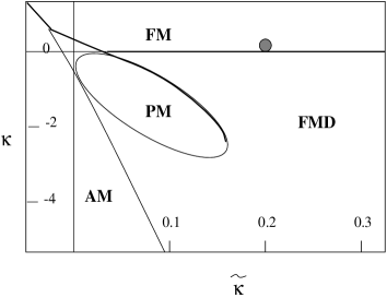
Figure 1: Schematic quenched phase diagram

where $\Box(U)$ is the covariant lattice laplacian and

$$B_{x}=\sum_{\mu}\left(\frac{V_{\mu x-\hat{\mu}}+V_{\mu x}}{2}\right)^{2}$$ (5)

with $V_{\mu x}=\frac{1}{2i}\left(U_{\mu x}-U_{\mu x}^{\dagger}\right)$ and $\tilde{\kappa}=1/(2\xi g^{2})$. $S_{gf}$ has a unique absolute minimum at $U_{\mu x}=1$, validating weak coupling perturbation theory (WCPT) around $g=0$ or $\tilde{\kappa}=\infty$ and in the naive continuum limit it reduces to $\frac{1}{2\xi}\int d^{4}x(\partial_{\mu}A_{\mu})^{2}$.

Obviously, the action $S_{B}(U)$ is not gauge invariant. By giving it a gauge transformation the resulting action $S_{B}(\phi^{\dagger}_{x}U_{\mu x}\phi_{x+\hat{\mu}})$ is gauge-invariant with $U_{\mu x}\rightarrow g_{x}U_{\mu x}h^{\dagger}_{x+\hat{\mu}}$ and $\phi_{x}\rightarrow g_{x}\phi_{x}$, $g_{x}\in U(1)$. By restricting to the trivial orbit, we arrive at the so-called reduced model action

$$S_{reduced}=S_{F}(U=1)+S_{B}(\phi^{\dagger}_{x}\;1\;\;\phi_{x+\hat{\mu}})$$ (6)

where $S_{B}(\phi^{\dagger}_{x}\;1\;\;\phi_{x+\hat{\mu}})$ now is a higher-derivative scalar field theory action.

3 Results in the Reduced Model

In the quenched approximation, we have first numerically confirmed the phase diagram in [3] of the model in ($\kappa,\tilde{\kappa}$) plane. The phase diagram shown schematically in Fig.1 has the interesting feature that for large enough $\tilde{\kappa}$, there is a continuous phase transition from FM to FMD phase. FMD phase is characterised by loss of rotational invariance and the continuum limit is to be taken from the FM side of the transition. In the full theory with dynamical gauge fields, the gauge symmetry reappears at this transition and the gauge boson mass vanishes, but the longitudinal gauge dof remain decoupled.

Figure 2: $RR$-propagator at antidomain wall ($L_{s}=22$; a.p.b.c. in $L_{4}$)

For calculating the fermion propagators, we have chosen the point $\kappa=0.05$, $\tilde{\kappa}=0.2$ (gray blob in Fig.1). Numerically on $4^{3}16$ and $6^{3}16$ lattices with $L_{s}=22$ we look for chiral modes at the domain wall ($s=0$), the antidomain wall ($s=11$), and at the $WG$ boundaries ($s=5,6$ and $s=16,17$). Error bars in Figs.2 and 3 are smaller than the symbols. Fig.2 shows the $RR$-propagator $|S_{RR}|$ at $s=11$ as a function of a component of momentum $p_{4}$ for both $\vec{p}=(0,0,0)$ (physical mode) and $(0,0,\pi)$ (first doubler mode) at different $y$-couplings. From the figure, it is clear that the doubler does not exist and the physical $RR$-propagator seems to have a pole at $p=(0,0,0,0)$. The curve stays the same irrespective of $y$-coupling and lattice size. We have also checked that it coincides exactly with the free $RR$-propagator (corresponding to $y\phi=1$) at $s=11$. Also similar analysis with the $LL$-propagator at $s=11$ does not show any pole. We conclude that there is only a free RH fermion at the antidomain wall. From similar data not shown here, we conclude that at the domain wall, there is a only free LH fermion.

Figure 3: $LL$-propagator at waveguide boundary ($L_{s}=22$, a.p.b.c. in $L_{4}$)

Fig.3 shows the $LL$ propagator at $s=6$ (waveguide boundary, just inside). Here too doublers do not exist. While there is a hint of a pole for $y=0.07$, the data for $y=0.5,~{}1.5$ does not favor any pole at zero momentum. Taking all our numerical data into account for the boundary propagators, there does not seem to exist any chiral modes there for $y\sim 1$. For very small $y$ the situation is tricky, because strictly at $y=0$, there are mirror boundary modes present, as can be seen from considerations of fermion current in $s$-direction and also from numerical simulation. We have done WCPT around $\tilde{\kappa}=\infty$ and $y=1$ and it supports the numerical data for $y\sim 1$.

In spite of having the longitudinal gauge dof explicitly in the action, it seems that in the reduced model we end up only with free undoubled chiral fermions at the domain wall and the antiwall with no mirror modes at the $WG$ boundaries.

References

- [1] M.F.L. Golterman and Y. Shamir, Phys. Lett. B399. (1997) 148.
- [2] M.F.L. Golterman, K. Jansen, D.N. Petcher and J.C. Vink, Phys. Rev. D49 (1994) 1606.
- [3] W. Bock et.al., Nucl.Phys.B (Proc.Suppl.) 63(1998)147; Phys.Rev.Lett 80(1998)3444.