Abelian hard thermal loops on a lattice

Abstract

In Abelian theories, one can write for the hard thermal loop equations of motions a local formulation that is more economical than the traditional Vlasov formulation and is in explicitly canonical form. I show how this formulation can be used for simulating non-equilibrium dynamics in the Abelian Higgs model.

1 HARD THERMAL LOOPS

Understanding the behaviour of quantum fields out of equilibrium is important both for cosmology and for heavy ion theory. A particularly interesting example of an event in the early universe in which out-of-equilibrium dynamics played a crucial role is the electroweak phase transition, since it may explain the observed baryon asymmetry in the Universe [1]. Although static equilibrium properties such as the phase structure of the theory have been determined to high accuracy with numerical lattice simulations [2], very little is known about the non-equilibrium behaviour. The reason is simply that while static correlators are given by a Euclidean path integral, which is well-suited for Monte Carlo simulations, one needs to evaluate a Minkowskian path integral to obtain any real-time correlator.

In the case of the electroweak phase transition, we can safely assume that the fields are in thermal equilibrium before the transition. The occupation number of the soft modes (with momentum $k\ll T$) is large, and a classical approximation can be used for them [3]. On the other hand, the hard modes ($k\mathop{\raise 1.29167pt\hbox{$>$\kern-7.5pt\raise-4.73611pt\hbox{$\sim$}}}T$) have a small occupation number and must be treated as quantum fields. Perturbation theory works well for the hard modes, and we can integrate out them perturbatively, constructing a classical effective theory for the soft modes [4]. This construction is free of infrared problems, since the loop integrals have an infrared cutoff, namely the ultraviolet cutoff $\Lambda$ of the effective theory. This approach has previously been used to measure the sphaleron rate of hot SU(2) gauge theory [4, 5]. It can also be used for simulating non-equilibrium dynamics of phase transitions, since the phase of the theory is a property of the soft modes only, and the distribution of the hard modes does not change in the transition.

At one-loop level, the resulting classical theory is simply the hard thermal loop effective theory. In high-temperature approximation and neglecting the IR cutoff in the loop integrals, we end up in the expression [6]

$${\cal L}_{\rm HTL} = -\frac{1}{4}F_{\mu\nu}F^{\mu\nu}$$ (1)

$$-\frac{1}{4}m_{D}^{2}\int\frac{d\Omega}{4\pi}F^{\mu\alpha}\frac{v_{\alpha}v^{\beta}}{(v\cdot\partial)^{2}}F_{\mu\beta}$$

$$+|D_{\mu}\phi|^{2}-m_{T}^{2}|\phi|^{2}-\lambda|\phi|^{4},$$

where $m_{D}^{2}=\frac{1}{3}e^{2}T^{2}$, $m_{T}^{2}=m^{2}+(e^{2}/4+\lambda/3)T^{2}$, and the integration is taken over the unit sphere of velocities $v=(1,\vec{v})$, $\vec{v}^{2}=1$. The time evolution of the fields is given by the equations of motion

$$\partial_{\mu}F^{\mu\nu} \!=\! m_{D}^{2}\int\!\frac{d\Omega}{4\pi}\frac{v^{\nu}v^{i}}{v\cdot\partial}E^{i}-2e{\rm Im}\phi^{*}D^{\nu}\phi,$$ (2)

$$D_{\mu}D^{\mu}\phi \!=\! -m_{T}^{2}\phi-2\lambda(\phi^{*}\phi)\phi.$$ (3)

Because of the derivative in the denominator, the gauge field equation of motion is non-local: the field interacts with fields on its whole past light cone.

2 LOCAL FORMULATION

To make numerical simulations practical, one needs a local formulation for the theory. For non-Abelian theories, two such formulations have been proposed: adding a large number of charged point particles [4] and introducing an extra field $W$, which satisfies the non-Abelian Vlasov equation [5, 7]. In practice, both of them lead to a 5+1-dimensional field theory. However, we will use the formulation presented in Ref. [8], where it was shown that in the Abelian case one can integrate out one of the dimensions, thus obtaining a 4+1-dimensional theory that is completely equivalent with the others. It consists of two extra fields $\vec{f}(t,\vec{x},z)$ and $\theta(t,\vec{x},z)$, where $z\in[0,1]$. In the temporal gauge, they satisfy the equations of motion

$$\partial_{0}^{2}{\vec{f}}(z) = z^{2}\vec{\nabla}^{2}\vec{f}+m_{D}z\sqrt{\frac{1-z^{2}}{2}}\vec{\nabla}\times\vec{A},$$ (4)

$$\partial_{0}^{2}{\theta}(z) = z^{2}\vec{\nabla}\cdot\left(\vec{\nabla}\theta-m_{D}\vec{A}\right),$$ (5)

$$\partial_{0}^{2}{\vec{A}} = -\vec{\nabla}\times\vec{\nabla}\times\vec{A}+m_{D}\int_{0}^{1}dzz^{2}\left(\vec{\nabla}\theta\right.$$ (6)

$$\left.-m_{D}\vec{A}+\sqrt{\frac{1-z^{2}}{2z^{2}}}\vec{\nabla}\times\vec{f}\right)+\vec{j}.$$

It is now possible to calculate any real-time correlator at finite temperature. One simply takes a large number of initial configurations from the thermal ensemble (the explicit form of the Hamiltonian was given in Ref. [8]), and evolves each of them in time, measuring the correlator of interest. The average over the initial configurations gives the ensemble average of the correlator. In principle, that approximates the corresponding expectation value in the original quantum theory to leading order in gauge coupling constant. In practice, one has to worry about some technical issues concerning the lattice cutoff that have been discussed in Refs. [4, 5, 7, 8, 9].

3 SIMULATIONS

To simulate the theory numerically, we discretize it by putting it on a lattice [8]. We expand $\vec{f}$ and $\theta$ in terms of Legendre polynomials:

$$\vec{f}^{(n)} = \int_{0}^{1}dzz\sqrt{\frac{2}{1-z^{2}}}P_{2n}(z)\vec{f}(z),$$

$$\theta^{(n)} = \int_{0}^{1}dzP_{2n}(z)\theta(z),$$ (7)

In addition to equilibrium real-time correlators, this formalism can be used to simulate out-of-equilibrium phenomena, such as the dynamics of the first-order phase transition [10] at $\lambda\ll e^{2}$. We do this in three steps:

1. We thermalize the soft modes to $T>T_{c}$ with a Monte Carlo simulation.

2. We decrease the temperature to slightly below $T_{c}$, and perform a smaller number of sweeps and generate the hard modes around the soft background. Since we use only local updates, the system does not tunnel to the true minimum, i.e., the Higgs phase, but remains in the Coulomb phase.

3. We solve numerically the equations of motion using the configuration obtained in step 2 as an initial configuration.

As an example, we show in Fig. 1 how the winding number density changes during the phase transition. Initially, the system is full of fluctuating strings, but after some time, some bubbles of the Higgs phase form and start to expand. The bubbles collide and strings are trapped between them. This is an example of the Kibble mechanism [11]. With the technique presented here, we can measure the properties of the resulting string networks and compare them with estimates based on non-gauged theories.

This approach can also be used to study various other properties of the phase transition. One of the most interesting quantities is the bubble nucleation rate. It can be measured in a straightforward way by taking a large number of initial configurations from the supercooled Coulomb phase and evolving each of them in time. If we plot the number of runs still remaining in the symmetric phase after time $t$, we get an exponentially decreasing curve, whose exponent gives the nucleation rate. This can be compared with the analytical results [12] to see, how well the analytical calculation really works in gauge theories.

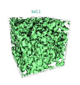
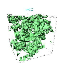
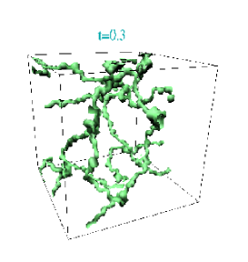
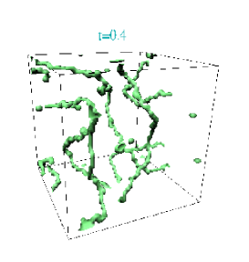
Figure 1: Time evolution of the winding number density during the course of a first-order phase transition.

References

- [1] V. A. Rubakov and M. E. Shaposhnikov, Usp. Fiz. Nauk 166, 493 (1996) [hep-ph/9603208].
- [2] K. Kajantie, M. Laine, K. Rummukainen, and M. Shaposhnikov, Nucl. Phys. B493, 413 (1997) [hep-lat/9612006].
- [3] D. Y. Grigoriev and V. A. Rubakov, Nucl. Phys. B299, 67 (1988).
- [4] C. R. Hu and B. Müller, Phys. Lett. B409, 377 (1997) [hep-ph/9611292]; G. D. Moore, C. Hu, and B. Müller, Phys. Rev. D58, 045001 (1998) [hep-ph/9710436].
- [5] D. Bödeker, G. D. Moore and K. Rummukainen, hep-ph/9907545.
- [6] U. Kraemmer, A. K. Rebhan, and H. Schulz, Ann. Phys. 238, 286 (1995) [hep-ph/9403301].
- [7] E. Iancu, Phys. Lett. B435, 152 (1998) [hep-ph/9710543]; hep-ph/9809535.
- [8] A. Rajantie and M. Hindmarsh, to appear in Phys. Rev. D, [hep-ph/9904270].
- [9] D. Bödeker, L. McLerran, and A. Smilga, Phys. Rev. D52, 4675 (1995) [hep-th/9504123].
- [10] K. Kajantie, M. Karjalainen, M. Laine, and J. Peisa, Nucl. Phys. B520, 345 (1998) [hep-lat/9711048].
- [11] T. W. B. Kibble, J. Phys. A9, 1387 (1976).
- [12] W. Buchmuller, T. Helbig and D. Walliser Nucl. Phys. B407, 387 (1993)