Improved Multiboson Algorithm

Abstract

We compare the performance of an UV-filtered Multiboson algorithm, including a global quasi-heatbath update, to the standard Hybrid Monte Carlo algorithm in full QCD with two flavours of Wilson fermions.

1 Introduction

In this study we consider QCD with two degenerate flavours of dynamical Wilson fermions. The partition function is given by

$${\mathcal{Z}}=\int\prod_{x,\mu}dU_{x,\mu}~{}e^{-S_{g}[U]}~{}\det(\mbox{$D$\kern-6.49994pt\hbox{/}\hskip 2.5pt}[U]+m)^{2}\quad.$$ (1)

The fermion determinant which results after integration of the fermions leads to non-local interactions among the gauge links $U_{x,\mu}$ making the cost for updating all links grow naively like ${\mathcal{O}}(V^{2})$, where $V$ is the lattice volume.

In the Hybrid Monte Carlo (HMC) algorithm, which is the standard method of numerical simulations with dynamical fermions, one uses an auxiliary bosonic pseudo-fermion field $\phi$ to write the determinant as

$$|\det(\mbox{$D$\kern-6.49994pt\hbox{/}\hskip 2.5pt}+m)|^{2}=\int[d\phi^{\dagger}][d\phi]~{}e^{-|(\not\kern-0.20999ptD+m)^{-1}\phi|^{2}}$$ (2)

and then uses Molecular Dynamics to globally update the $U$.

An alternative approach, which allows the use of local algorithms, is the Multiboson (MB) method, originally proposed by Lüscher [2]. A polynomial $P_{n}(x)=c_{n}\prod_{k=1}^{n}(x-z_{k})$ is constructed which approximates $1/x$ over the whole spectrum of $(\mbox{$D$\kern-6.49994pt\hbox{/}\hskip 2.5pt}+m)$. Then $P_{n}(\mbox{$D$\kern-6.49994pt\hbox{/}\hskip 2.5pt}+m)\approx(\mbox{$D$\kern-6.49994pt\hbox{/}\hskip 2.5pt}+m)^{-1}$ and one can write

$$|\det(\mbox{$D$\kern-6.49994pt\hbox{/}\hskip 2.5pt}+m)|^{2}\approx|{\det}^{-1}P_{n}(\mbox{$D$\kern-6.49994pt\hbox{/}\hskip 2.5pt}+m)|^{2}$$ (3)

$$=c_{n}^{-2V}\int\prod_{k}[d\phi_{k}^{\dagger}][d\phi_{k}]~{}e^{-\sum_{k}|(\not\kern-0.20999ptD+m-z_{k})\phi_{k}|^{2}}\quad.$$

In this way the original QCD partition function is written approximately in terms of a local action so that standard powerful local algorithms (heatbath, overrelaxation) can be used. The systematic error deriving from this approximation can be corrected either during the simulation, with a global accept-reject step, or by a reweighting procedure on physical observables.

We compare here the efficiency of an improved version of the MB algorithm with a “state of the art” HMC algorithm, namely the one used by the SESAM collaboration [3]. The observables used for this comparison are the plaquette, representative of the smallest (UV) scale, and the topological charge, representative of the largest (IR) scale features of the gauge field.

2 Algorithm

We use the exact, non-hermitian version of the MB algorithm [4] with a noisy Metropolis test to correct for the polynomial approximation to the fermionic determinant. There exist two different, complementary strategies for improving the efficiency of the MB method:
1.UV-filtering: The first is the choice of an optimal polynomial $P_{n}$ which keeps $n$ as low as possible and still achieves a reasonable Metropolis acceptance. We follow the procedure of [5] inspired by the loop expansion of the fermion determinant: ${\rm det}({\bf 1}-\kappa M)=e^{-\sum_{j}a_{j}{\rm Tr}M^{j}}\times{\rm det}\left(({\bf 1}-\kappa M)~{}~{}e^{+\sum_{j}a_{j}M^{j}}\right)$. We group the term $e^{-\sum_{j}a_{j}{\rm Tr}M^{j}}$ with the gauge action (for $j\leq 4$ this amounts to a mere shift in $\beta$) and find a polynomial approximation to the inverse of $({\bf 1}-\kappa M)~{}~{}e^{+\sum_{j}a_{j}M^{j}}$. The parameters have to be chosen so that $\det W\simeq 1$, where $W\equiv\prod_{k}^{n}({\bf 1}-\kappa M-z_{k}{\bf 1})\cdot({\bf 1}-\kappa M)\cdot e^{\sum_{j=0}^{m-1}a_{j}M^{j}}$. A sufficient condition for this is that $W\eta\simeq\eta$ for Gaussian vectors $\eta$. Therefore one takes an equilibrium gauge configuration, fixes the coefficients $a_{j}$ to some initial value, draws one or more Gaussian vectors $\eta$ and finds, by quadratic minimization, the roots $\{z_{k}\}$ which minimize the quantity $e=\parallel W\eta-\eta\parallel^{2}$. The derivatives $\partial e/\partial a_{j}$ are also obtained, which allows the optimization of both the coefficients $\{a_{j}\}$ and the zeros $\{z_{k}\}$, following ref. [5].
2.Quasi - heatbath: The second is the choice of the update algorithm for gauge links and boson fields. The coupled dynamics of the system (gauge links + boson fields) is highly non trivial, so that the optimal mixture of update algorithms is essentially determined by numerical experiment [6]. For light quark masses one needs a good algorithm to speed up the IR bosonic modes. To implement a global heatbath on the bosonic fields one must assign $\phi_{k}^{\rm NEW}=(D-z_{k})^{-1}\eta$ where $D=1-\kappa M$ and $\eta$ is a Gaussian random vector. This procedure is expensive especially for small quark masses. Instead we use a quasi-heatbath consisting of an approximate inversion plus a Metropolis accept-reject step as proposed in [7]. i.e. we solve approximately $(D-z_{k})x=(D-z_{k})\phi_{k}^{\rm OLD}+\eta$ and set $\phi_{k}^{\rm NEW}=x-\phi_{k}^{\rm OLD}$. We then accept with probability

$$min\left(1,{\rm exp}(2Re(r^{\dagger}.(D-z_{k})(\phi_{k}^{\rm NEW}-\phi_{k}^{\rm OLD})\right)$$ (4)

with $r$ the residual. We combine this global update with local overrelaxation of gauge and bosonic fields.

3 Results

Three representative systems, denoted (A),(B) and (C), in Table I, have been studied: medium-heavy quarks in a small lattice, light quarks in a small lattice, and light quarks in a large lattice. The HMC simulations used for comparisons of these systems incorporate state-of-the-art improvements (but without the recently implemented SSOR preconditioning).

Simulation	A	B	C
Volume	$8^{4}$	$8^{4}$	$16^{3}\times 24$
$\beta,\kappa$	$5.3,0.158$	$5.3,0.165$	$5.6,0.156$
$n_{bosons}$	7	16	24
$a_{2}$	1.389	6.066	4.077
$a_{4}$	4.411	4.423	8.789
$\Delta\beta=192\kappa^{4}a_{4}$	0.527	0.629	0.999
$\tau_{int}(\Box)(MB)$	$\sim 3500$	$\sim 64000$	$\sim 27500$
$\tau_{int}(\Box)(HMC)$	$\sim 14000$	$\sim 72000$	$\sim 85000$

Table 1: Summary of the parameters of our 3 simulations. Integrated autocorrelation times are measured in units of applications of the Wilson Dirac matrix to a vector.

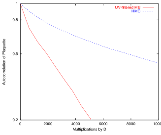
Figure 1: Autocorrelation of the plaquette, with the UV-filtered MB algorithm (solid line) and the HMC algorithm (dashed line) at $\beta=5.3$ and $\kappa=0.158$ (simulation A).

Medium - heavy quarks on a small lattice (Simulation A): Only seven bosonic fields are required, with only one zero $z_{k}$ devoted to the UV part of the Dirac spectrum. As demonstrated in Fig. 1 the plaquette decorrelates about 4 times faster than with HMC.

Light quarks on a small lattice (Simulation B): To see if there is a quark mass below which the MB loses its advantage we consider light quarks. Several of the IR zeros are now closer to the Dirac spectrum boundary. The quasi-global heatbath provides an improvement of at least a factor of 5. From the plaquette autocorrelation the HMC and MB algorithms appear equally efficient.

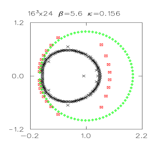
Figure 2: Zeros of the UV-filtered polynomial ($n=24$, squares), of the non-UV-filtered polynomial ($n=80$, diamonds), and estimated boundary of the Dirac spectrum (x), (simulation C).

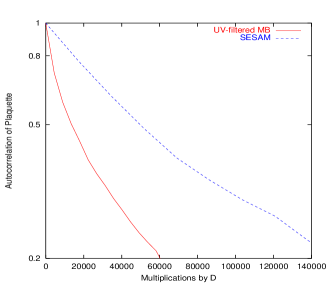
Figure 3: Autocorrelation of the plaquette, with the UV-filtered MB algorithm (solid line) and the SESAM HMC algorithm (dashed line) at $\beta=5.6$ and $\kappa=0.156$ (simulation C).

Light quarks on a large lattice (Simulation C): The number of boson fields needed is 24, as compared with 80 which would have been needed with no UV-filtering for a comparable acceptance. Fig. 2 shows that 16 of the roots of the UV-filtered polynomial are devoted to the IR modes and 8 to the UV modes of the Dirac operator.

Figure 4: Comparison of topological charge histories obtained with HMC and UV-filtered MB algorithm at $\beta=5.6$ and $\kappa=0.156$. The common scale has been set in terms of equivalent $D\times v$ multiplications.

The autocorrelation of the plaquette is compared in Fig. 3 with that obtained by the SESAM collaboration using HMC [3]. Our MB approach is more efficient by a factor $\sim 3$. In Fig. 4 we compare the topological charge histories obtained from our simulation and from a sample of SESAM configurations [8]. In both cases the same cooling method was used. Neither simulation is long enough to extract a reliable autocorrelation time for this observable. Attempts at doing so yield roughly equivalent results for both algorithms, as the figure already indicates. Therefore, even for this global observable, our MB method seems not worse than HMC.

4 Conclusions

The numerical evidence presented in this study shows that the non-hermitian MB algorithm with UV-filtering and a global quasi-heatbath of the boson fields is a superior alternative to the traditional HMC: it decorrelates the plaquette more efficiently, and the topological charge equivalently well.

References

- [1]
- [2] M. Lüscher, Nucl. Phys. B418 (1994) 637.
- [3] SESAM collaboration, Th. Lippert et al., Nucl. Phys. (Proc. Suppl.) B63 (1998) 946.
- [4] A. Borrelli et al., Nucl. Phys. B477 (1996)809.
- [5] Ph. de Forcrand, Nucl. Phys. (Proc.Suppl.) B73 (1999) 822.
- [6] B. Jegerlehner, Nucl. Phy. B465 (1996) 487.
- [7] Ph. de Forcrand, Phys. Rev. E 59 (1999) 3698.
- [8] B. Allés et al., Phys. Rev. D58 (1998) 071503.