Quantum gauge fixing and vortex dominance UNITU-THEP 11/99

Abstract

We introduce quantum gauge fixing (QGF) as a new class of gauge fixings. While the maximal center gauge might not show vortex dominance, the confining properties of the vortices observed in past lattice calculations are argued to have been obtained in a gauge more akin to QGF than to the strict maximal center gauge.

1 Introduction

In recent years, evidence has been accumulated that the mechanism of quark confinement may be understood in effective theories of monopoles [1, 2] or $Z_{N}$ vortices [3]-[6]. After gauge fixing, these theories arise from projecting the full SU(N) onto a gauge theory with a reduced gauge symmetry. The observation that the reduced theories reveal the full string tension nurtures the conjecture that those degrees of freedom bear confinement. Here, we will employ center gauge fixing and center projection [3] for the reduction of SU(2) to $Z_{2}$ gauge theory which can be understood as a theory of vortices. We define vortex dominance if two criteria are met. Firstly, the string tension is preserved by projection. Secondly, the vortices survive the continuum limit.

2 Center gauge fixing (standard)

Let $U_{\mu}(x)$ denote the link variable of SU(2) gauge theory and $\Omega(x)$ a gauge transformation matrix. Maximizing the functional

$$S_{fix}[U]=\sum_{\{x\}\mu}\frac{1}{2}{\rm tr}\left\{U^{\Omega}_{\mu}(x)\,\tau^{a}\,U^{\Omega\,\dagger}_{\mu}(x)\,\tau^{a}\right\}\;,$$ (1)

with respect to $\Omega(x)$ yields the gauge transformation matrices which, when applied, cast a given configuration in the center gauge. Center projection is performed by the mapping of the link variable $U^{\Omega}(x)$ onto ${\pm 1}$ (see e.g. [3]).

In practical calculations, finding the absolute maximum of the functional $S_{fix}$ is a difficult task. The results which are presented in the next section were obtained by applying the algorithm presented in [3], which resorts to iteration with over-relaxation. Once the iteration does not change the functional $S_{fix}$ any more up to a given precision, we performed a random gauge transformation on the actual link configuration and repeat the center gauge fixing. The procedure is repeated up to ten times. We finally choose the configuration $\Omega(x)$ which corresponds to the maximum value within the series of the ten fixing steps. This alleviates, but does not eliminate, the Gribov problem (see section 4).

3 Numerical results

Zero temperature: It turns out that the effective $Z_{2}$ gauge theory which was constructed with the ITOV-algorithm sketched above shows vortex dominance: the string tension is preserved [3, 5], and the linking number of the vortex lines with a Wilson loop (vortex density) meets with the expectations from a renormalization group analysis [6]. Also the vortex interactions scale. These observations suggest that the vortices are physical objects surviving the continuum limit [6].

Figure 1: Distribution of the vortex cluster sizes; ”1” is the maximum length possible in the lattice universe.

Finite temperatures: We find that below the deconfinement temperature $T_{c}$ vortex dominance persists [7]. In particular, the effective $Z_{2}$ gauge theory correctly reproduces the critical temperature thus indicating that the essence of the deconfinement phase transition can be captured in the vortex picture. A thorough study of the density of vortices which are linked to spatially oriented Wilson loops shows that the vortex state at high temperatures is in agreement with the predictions of dimensional reduction [7]. On the other hand, the density of vortices linked with time-like Wilson loops only drops by a factor of three if the temperature is raised to twice $T_{c}$. Additional information is needed to understand the drop of the string tension to zero at $T_{c}$. We argue [7, 8] that while the vortices are organized in a huge cluster at zero temperature, they stop percolating at $T_{c}$ and the huge cluster decays into many small size clusters. If in the later case the size of the Wilson loop exceeds the average cluster size, only vortices close to the circumference of the Wilson loop contribute yielding a perimeter law. In order to substantiate this idea, we measured the probability that a link of the vortex belongs to a cluster of given size. The result is depicted in figure 1. Further details can be found in [8].

4 Gribov ambiguities

The variety of results in the previous section was obtained by implementing the center gauge (see (1)) with the help of the ITOV algorithm sketched in section 2. It was recently pointed out that this procedure does not evade the Gribov problem [9]. In fact, it was observed that implementing the Landau gauge before applying the ITOV algorithm leads on average to a larger maximum value of $S_{fix}$ (1) than attained by the direct use of the ITOV algorithm. Moreover, the vortex state constructed from the gauge fixing via the Landau gauge detour does not show vortex dominance. These results cast doubt on the issue of vortex dominance in the strict maximal center gauge and call for a more accurate specification of the gauge in which the results outlined in section 3 were really obtained.

5 Quantum gauge fixing

For this specification, we here propose a new type of gauge fixing procedure which we will call Quantum gauge fixing (QGF). We will argue that the ITOV algorithm of section 2 already contains some of the characteristics of QGF rather than representing a numerically stable implementation of the maximal center gauge. Defining the $SU(N)/Z_{N}$ matrices

$$\zeta_{ab}(x) := \frac{1}{2}{\rm tr}\left\{\Omega(x)\,\tau^{a}\,\Omega^{\dagger}(x)\,\tau^{b}\right\}\;,$$ (2)

$$R^{\mu}_{ab}(x) := \frac{1}{2}{\rm tr}\left\{U_{\mu}(x)\,\tau^{a}\,U_{\mu}^{\dagger}(x)\,\tau^{b}\right\}\;,$$ (3)

the gauge fixing functional $S_{fix}$ (1) can be cast into

$$S_{fix}\;=\;\sum_{\{x\}\mu}\;{\rm tr}\;\zeta^{T}(x+\mu)\,R^{\mu}(x)\,\zeta(x)\;.$$ (4)

Center gauge fixing corresponds to maximizing (4) with respect to the matrices $\zeta$ for a given lattice configuration, i.e., $R^{\mu}(x)$. From given matrices $\zeta(x)$, the gauge transformation $\Omega(x)$ can be constructed up to a center gauge transformation,

$$f^{Z}_{SU}:\;SU(N)/Z_{N}\rightarrow SU(N):\;\Omega=f^{Z}_{SU}(\zeta)\;.$$ (5)

This ambiguity reflects the familiar fact that the maximal center gauge condition leaves a residual $Z_{N}$ gauge group unfixed.

We define the QGF as follows: by means of a functional integral over gauge transformations $\zeta$, we construct the matrix

$$\omega[U]\;:=\;\frac{1}{N}\int{\cal D}\zeta\;f^{Z}_{SU}(\zeta)\;\exp\left\{\beta_{f}\,S_{fix}\right\}\;,$$ (6)

which in general is not an element of the gauge group. The gauge transformation $\Omega(x)$ which brings a given field configuration $U_{\mu}(x)$ into the quantum gauge is then defined by the SU(N) element ”closest” to $\omega[U]$, i.e.,

$$||\,\omega[U](x)-\Omega(x)\,||^{2}\rightarrow\hbox{min}\;,\;\;\;\forall\,x\;,$$ (7)

where $||A||^{2}:={\rm tr}AA^{\dagger}$. It can be shown that the QGF (6-7) is free of Gribov ambiguities. In the case of the center gauge fixing (4), the functional integral in (6) can be viewed as a partition function of the matrices $\zeta$ each interacting with its nearest neighbors via the metric $R^{\mu}(x)$. This quantum theory of matrices $\zeta$ is therefore interpreted as generalized spin glass. Spin glass systems are known for a complex phase structure. A numerical calculation of the expectation value (6) is therefore tedious, and we recover the Gribov problem in practical applications.

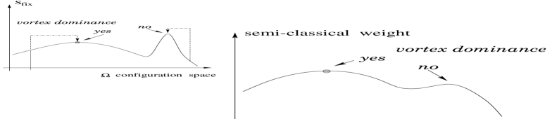
Figure 2: The illustration of $S_{fix}$ and the semi-classical weight (8) as functional of $\zeta(x)$.

Nevertheless, QGF is helpful to put the results outlined in section 3 in the proper context. For this purpose, we consider large values of the gauge parameter $\beta_{f}$ in (6). In this case, the configuration $\zeta(x)$ which corresponds to a local maximum of $S_{fix}$ contributes to $\omega$ with the (semi-classical) weight

$$\propto\,\exp\left\{\beta_{f}S_{fix}\left[\zeta\right]\right\}\,/\,\left[S^{\prime\prime}_{fix}\left[\zeta\right]\right]^{1/2}\;,$$ (8)

where $S^{\prime\prime}_{fix}$ is the functional determinant of the second (functional) derivative of $S_{fix}$ with respect to $\zeta(x)$. Eq.(8) implies that the contributions of maxima with large curvature are suppressed. The situation is illustrated in figure 2. Since the ITOV algorithm of section 2 involves several steps of iteration which start with a random choice of $\zeta$, it probes the volume of the region of attraction corresponding to a particular maximum. The ITOV algorithm therefore effectively contains a similar entropy factor as the one implied by (6). We therefore argue that the results shown in section 3 refer to a gauge which is more akin (but not completely identical) to QGF than to the strict maximal center gauge.

Supported in part by DFG-RE 856/4-1, DFG-En 415/1-1.

References

-
[1]
Y. Nambu, Phys. Rev. D 10 (1974) 4262;
G. ’t Hooft, in: High Energy Physics, ed. A. Zichichi, Bologna, 1975;
S. Mandelstam, Phys. Rep. B 23 (1976) 245. -
[2]
K. Schilling, G.S. Bali and C. Schlichter,
Nucl. Phys. Proc. Suppl. 73 (1999) 638.
A. Di Giacomo, B. Lucini, L. Montesi and G. Paffuti, hep-lat/9906024. -
[3]
L. Del Debbio, M. Faber, J. Giedt, J. Greensite and S. Olejnik,
Phys. Rev. D58 (1998) 094501;
L. Del Debbio, M. Faber, J. Greensite and S. Olejnik, Nucl. Phys. Proc. Suppl. 53 (1997) 141. -
[4]
G. ’t Hooft, Nucl. Phys. B138 (1978) 1;
G. Mack, in: Recent Developments in Gauge Theories, eds. G. ’t Hooft et al (Plenum, New York, 1980). - [5] L. Del Debbio, M. Faber, J. Greensite and S. Olejnik, Phys. Rev. D55 (1997) 2298.
-
[6]
K. Langfeld, H. Reinhardt and O. Tennert,
Phys. Lett. B419 (1998) 317;
M. Engelhardt, K. Langfeld, H. Reinhardt and O. Tennert, Phys. Lett. B431 (1998) 141. - [7] K. Langfeld, O. Tennert, M. Engelhardt and H. Reinhardt, Phys. Lett. B452 (1999) 301.
- [8] M. Engelhardt, K. Langfeld, H. Reinhardt and O. Tennert, hep-lat/9904004.
- [9] T. G. Kovacs, E. T. Tomboulis, hep-lat/9905029.