Casimir scaling or flux counting ? HUB-EP-99/44

Abstract

Potentials between two static sources in various representations of the SU(3) gauge group are determined on anisotropic $3+1$ dimensional lattices. Strong evidence in favour of “Casimir scaling” is found.

1 THE QUESTION

Static colour sources offer an ideal environment for investigating the confinement mechanism and testing models of low energy QCD. Despite the availability of a wealth of information on fundamental potentials [1, 2], only few lattice investigations of forces between sources in higher representations of the gauge group SU(N) exist. Most of these studies have been done in SU(2) gauge theory in three [3, 4] and four [5] space-time dimensions. Only two groups have obtained results for four dimensional SU(3) gauge theory so far, one of them at finite temperature from Polyakov lines [6] and the other from Wilson loops [7, 8] at zero temperature.

For the static potential in the singlet channel, tree level perturbation theory yields the result,

$$V_{D}(r)=-C_{D}\frac{g^{2}}{4\pi}\frac{1}{r},$$ (1)

where $D=1,3,6,8,10,\ldots$ labels the representation of SU(3). $D=3$ corresponds to the fundamental representation, $F$, and $D=8$ to the adjoint representation, $A$. $C_{D}$ labels the corresponding quadratic Casimir operator $C_{D}=\mbox{Tr}_{D}t_{a}^{D}t_{a}^{D}$ with the trace $\mbox{Tr}_{D}$ and generators $t^{D}_{a}$ obeying the normalisation conditions, $\mbox{Tr}_{D}{\mathbf{1}}_{D}=1$, $[t_{a}^{D},t_{b}^{D}]=if_{abc}t_{c}^{D}$. The Table below contains all representations $D$ that we have realised, the corresponding weights $(p,q)$ and the ratios of Casimir factors, $d_{D}=C_{D}/C_{F}$. In SU(3) we have $C_{F}=4/3$ and $z=\exp(2\pi i/3)$ denotes a third root of one.

$D$	$(p,q)$	$z^{p-q}$	$p+q$	$d_{D}$
3	$(1,0)$	$z$	1	1
8	$(1,1)$	1	2	2.25
6	$(2,0)$	$z^{*}$	2	2.5
$15a$	$(2,1)$	$z$	3	4
10	$(3,0)$	1	3	4.5
27	$(2,2)$	1	4	6
24	$(3,1)$	$z^{*}$	4	6.25
$15s$	$(4,0)$	$z$	4	7

We denote group elements in the fundamental representation of SU(3) by $U$. The traces of $U$ in various representations, $T_{D}=\mbox{tr}\,U_{D}$, can easily be obtained,

$$T_{3} = \mbox{tr}\,U,\quad T_{8}=\left(|T_{3}|^{2}-1\right),$$

$$T_{6} = \frac{1}{2}\left[(\mbox{tr}\,U)^{2}+\mbox{tr}\,U^{2}\right],$$

$$T_{15a} = \mbox{tr}\,U^{*}\,T_{6}-\mbox{tr}\,U,$$ (2)

$$T_{10} = \frac{1}{6}\left[(\mbox{tr}\,U)^{3}+3\,\mbox{tr}\,U\,\mbox{tr}\,U^{2}+2\,\mbox{tr}\,U^{3}\right],$$

$$T_{24} = \mbox{tr}\,U^{*}\,T_{10}-T_{6},\quad T_{27}=|T_{6}|^{2}-|T_{3}|^{2},$$

$$T_{15s} = \frac{1}{24}\left[(\mbox{tr}\,U)^{4}+6(\mbox{tr}\,U)^{2}\mbox{tr}\,U^{2}\right.$$

$$+ \left.3(\mbox{tr}\,U^{2})^{2}+8\,\mbox{tr}\,U\,\mbox{tr}\,U^{3}+6\,\mbox{tr}\,U^{4}\right].$$

Note the difference, $\mbox{Tr}_{D}U_{D}=\frac{1}{D}\mbox{tr}\,U_{D}=T_{D}/D$. Under the replacement $U\rightarrow zU$, $T_{D}\rightarrow z^{p-q}T_{D}$.

It is known [1, 2] that for distances $r=R/a_{s}\geq 0.6\,r_{0}\approx$ 0.3 fm the fundamental potential is well described by the parametrisation,

$$V_{F}(R)=V_{0,F}-\frac{e_{F}}{R}+K_{F}R.$$ (3)

Perturbation theory tells us, $V_{0,R}\approx d_{R}V_{0,F}$, $e_{R}\approx d_{R}e_{F}$. While the fundamental potential in pure gauge theories linearly rises ad infinitum, the adjoint potential will be screened by gluons and, at sufficiently large distance, decay into two gluelumps (or gluinoballs), bound states of a static adjoint source (gluino) and gluons. This string breaking has indeed been confirmed [4]. Therefore, strictly speaking, the adjoint string tension is zero. In fact, all charges in higher than the fundamental representation will be at least partially screened by the background gluons. For instance, $6\otimes 8=24\oplus 15a^{*}\oplus 6\oplus 3^{*}$: in interacting with the glue, the sextet potential obtains a fundamental component. However, in an intermediate range an approximate linear behaviour is found [3, 4, 5, 6, 7, 8], such that one might speculate whether in this region the Casimir scaling hypothesis $K_{D}\approx d_{D}K_{F}$ holds.

A simple rule, related to the centre of the group, is reflected in Eq. (2): where ever $z^{p-q}=1$, the source will be reduced into a singlet component at large distance while, where ever $z^{p-q}=z(z^{*})$, it will be screened up to a residual (anti-)triplet component, i.e. one can easily read off the asymptotic string tension ($0$ or $K_{F}$) from the third column of the Table, rather than having to multiply and reduce representations. If centre symmetry plays such a prominent rôle at infinite distance, one might imagine the intermediate distance slopes to count the number of fundamental flux tubes $p+q$ that are embedded into the higher representation vortex. This flux counting model is supported by indications that the QCD vacuum lies on the boundary between a type I and a type II superconductor [9] and, therefore, interactions between neighbouring vortices are weak. Indeed, latest results on the adjoint SU(2) potential [4] as well as on the octet and sextet SU(3) potentials [8] turn out to lie significantly lower than the expected Casimir ratios suggest. Expectations from both models, Casimir scaling and flux counting, at least for the lower dimensional representations, are close to each other, such that discriminating between them represents a numerical challenge.

2 THE METHOD

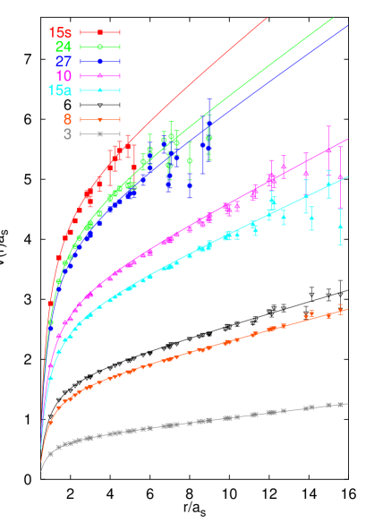
Figure 1: Static potentials between sources in various representations of SU(3).

We simulate SU(3) gauge theory on anisotropic lattices, using the standard plaquette action,

$$S=\beta\left(\frac{1}{\xi_{0}}\sum_{x,i>j}S_{x,ij}+\xi_{0}\sum_{x,i}S_{x,i4}\right).$$ (4)

We determine the renormalised anisotropy from the (fundamental) spatial potential, $a_{s}V_{s}(R_{s}a_{s})=a_{s}V_{s}(R_{t}a_{t})=a_{s}V_{s}(0.8\,r_{0})$. For the combination, $\beta=6.2$ and $\xi_{0}=3.25$, we find $\xi=a_{s}/a_{t}=R_{t}/R_{s}\approx 4$, $r_{0}\approx 6\,a_{s}$, i.e. ${a_{t}}^{-1}\approx 9.6$ GeV, $a_{s}^{-1}\approx 2.4$ GeV. We present only preliminary results from an analysis of a subset of our final statistics at these parameter values. Additional simulations are being performed at courser lattices with constant renormalised anisotropy.

The potentials are extracted in the standard way from fits to spatially smeared Wilson loops [1]. Wilson loops in higher representations are obtained from the fundamental one by use of Eq. (2). In SU(3), unlike in SU(2) [4], this procedure excludes thermal averaging of temporal links.

3 THE ANSWER

In Fig. 1, we display our results in lattice units, $a_{s}\approx 4\,a_{t}$. $r=12\,a_{s}$ corresponds to a distance $r\approx 1$ fm. Note, that we display the raw lattice data and have not subtracted any self energy piece. We fit the fundamental potential for distances $r\geq 0.6~{}r_{0}$ to Eq. (3). The expectations on the potentials $V_{D}(r)$, which are dispayed in the Figure, correspond to this fit curve, multiplied by the factors $d_{D}$. As one can see, up to distances where the signal disappears into noise or the string might break, the data is well described by the Casimir scaling assumption.

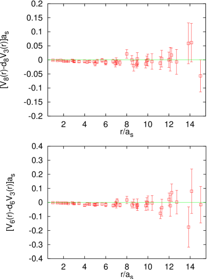
Figure 2: Test of the Casimir scaling hypothesis.

In Fig. 2, we have subtracted the fundamental potential, multiplied by the factors $d_{8}$ and $d_{6}$ from the adjoint and sextet potentials, respectively. We benefit from a reduction of statistical errors, due to correlations between the data sets. While the flux counting model is certainly ruled out, the Casimir scaling model tends to slightly overestimate the data points. For higher representations, the situation looks similar. Compared to results from coarser lattices [8] ($r_{0}\approx 3\,a$ as opposed to $r_{0}\approx 24\,a_{t}$) the disagreement, however, is vastly reduced and will eventually completely disappear in the continuum limit. A comprehensive study with proper extrapolation to the continuum limit is in preparation.

References

- [1] G.S. Bali and K. Schilling, Phys. Rev. D47 (1993) 661.
- [2] G.S. Bali, K. Schilling and A. Wachter, Phys. Rev. D56 (1997) 2566; ibid. D55 (1997) 5309.
- [3] J. Ambjorn, P. Oleson, and C. Peterson, Nucl. Phys. B240 (1984) 533; G.I. Poulis and H.D. Trottier, Nucl. Phys. B (Proc. Suppl.) 42 (1995) 267.
- [4] P.W. Stephenson, Nucl. Phys. B550 (1999) 427; O. Philipsen and H. Wittig, Phys. Lett. B451 (1999) 146.
- [5] J. Ambjorn, P. Oleson, and C. Peterson, Nucl. Phys. B240 (1984) 189; C. Michael, Nucl. Phys. B259 (1985) 58; L.A. Griffiths, C. Michael, and P.E.L. Rakow, Phys. Lett. 150B (1985) 196; H.D. Trottier, Phys. Lett. B357 (1995) 193.
- [6] H. Markum and M.E. Faber, Phys. Lett. B200 (1988) 343; M. Müller, W. Beirl, M. Faber, and H. Markum, Nucl. Phys. B (Proc. Suppl.) 26 (1992) 423.
- [7] N.A. Campbell, I.H. Jorysz, C. Michael, Phys. Lett. 167B (1986) 91; C. Michael, Nucl. Phys. B (Proc. Suppl.) 26 (1992) 417.
- [8] C. Michael, hep-ph/9809211.
- [9] G.S. Bali, hep-ph/9809351; G.S. Bali, K. Schilling and C. Schlichter, Prog. Theor. Phys. Suppl. 131 (1998) 645.