Improving the sign problem in QCD at finite density

Abstract

If the fermion mass is large enough, the phase of the fermion determinant of QCD at finite density is strongly correlated with the imaginary part of the Polyakov loop. This fact can be exploited to reduce the fluctuations of the phase significantly , making numerical simulations feasible in regions of parameters where the naive brute force method does not work.

1 The Polyakov loop and the phase of the determinant

It is well known that the euclidean path integral representation of the QCD partition function at finite chemical potential suffers from the so-called sign problem: the fermion determinant is complex and the theory cannot be simulated with the usual Monte Carlo method. One could still try to get results with the simple brute force method, that is, simulate a positive measure which contains the pure gauge action and the modulus of the determinant, treating the phase as an observable. Then, the expectation value of any observable $\cal{O}$ is given by the ratio $\langle{\cal O}\rangle=\langle{\cal O}\exp i\theta\rangle_{m}/\langle\cos\theta\rangle_{m}$, where $\langle\cdot\rangle_{m}$ denotes the expectation value using the modulus of the determinant as a probability measure, and $\theta$ is the phase of the determinant (PD). Unfortunately, the expectation value of $\cos\theta$ is a positive quantity exponentially small with the volume. Since the relative error $\langle{\cal O}\rangle$ is given by

$$\frac{\delta\langle{\cal O}\rangle}{\langle{\cal O}\rangle}=\frac{\delta\langle{\cal O}\exp i\theta\rangle_{m}}{\langle{\cal O}\exp i\theta\rangle_{m}}+\frac{\delta\langle\cos\theta\rangle_{m}}{\langle\cos\theta\rangle_{m}}\,,$$ (1)

$\langle\cos\theta\rangle_{m}$ must be measured very accurately to achieve a given accuracy for $\langle{\cal O}\rangle$. This requires statistic growing exponentially with the volume. Obviously, this is, from the numerical point of view, an almost hopeless task.

Due to the up to now unsurmountable difficulties with QCD with light quarks at finite density, increasing attention is being paid to the limit of infinitely heavy quarks [1]-[4]. The sign problem still remains in this limit, but numerical computations are easier [1]. For large quark mass $m$, the logarithm of the fermion determinant can be expanded in powers of $1/(2m)$ (we focus our discussion on staggered fermions). The first term sensitive to the chemical potential $\mu$ is

$$\left(\frac{e^{\mu}}{2m}\right)^{N_{T}}\,\sum_{\vec{x}}{\rm Tr}L_{\vec{x}}\>+\>\left(\frac{e^{-\mu}}{2m}\right)^{N_{T}}\,\sum_{\vec{x}}{\rm Tr}L_{\vec{x}}^{\dagger}\,,$$ (2)

where $N_{T}$ is the number of lattice points in the temporal direction, $\vec{x}$ labels the sites in a given temporal slice, and $L_{\vec{x}}$ is the ordered product of all temporal links attached to $\vec{x}$. Hence, to this order, the PD is proportional to the imaginary part of the Polyakov loop (IPPL): $\theta=cV_{s}L_{i}$, with $L_{i}=1/V_{s}\sum_{\vec{x}}{\rm ImTr}L_{\vec{x}}$ and $c=2\sinh(\mu N_{T})/(2m)^{N_{T}}$. Of course, higher order corrections will destroy this linear relationship.

The static limit ($m,\mu\rightarrow\infty$ with $c=[\exp(\mu)/2m]^{N_{T}}$ fixed) has been studied in [1]. Analyzing the data of [1], we found a strong correlation between the PD and the IPPL, as can be seen in Figs. 1 and 2 [4]. The strong correlation displayed in Fig. 1 is not surprising, since the data correspond to $c\approx 0.05$, which is small enough for the linear relation previously discussed to become essentially exact. Fig. 2 is more interesting, since $c\approx 1.66$ is not small. There, we can see that the linear correlation still holds, though the width of the band is much larger than in Fig. 1. Very recently, a paper confirming these findings from a continuum analysis has appeared [5].

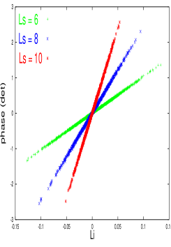
Figure 1: Correlation between The PD $\theta$ and The IPPL $L_{i}$ in static QCD, with $C=1/20$ and $\beta=5.0$ on a lattice $L_{s}^{3}\times 2$. The data are from Ref. 1.

2 Fixing the imaginary part of the Polyakov loop

Given the correlation between the PD and the IPPL, it is plausible that, at least for heavy enough quarks, the fluctuations of the PD would be suppressed to a large extent provided we constrain our path integral to configurations with real Polyakov loop. To see whether this is possible we write the partition function as ${\cal Z}=\int dp_{i}\,\exp\left(-V_{s}{\cal F}(p_{i})\right)$, where $V_{s}$ is the spatial lattice volume and

$$e^{-V_{s}{\cal F}}=\int[dU]e^{-S_{g}(U)}\det\Delta(U)\,\delta(p_{i}-L_{i})\,.$$ (3)

For $V_{s}\rightarrow\infty$ the integral in $p_{i}$ is saturated by the saddle point $p_{i}^{\textstyle\scriptscriptstyle sp}$, which is in general complex, since ${\cal F}$ is.

It is easy to show that the saddle point is indeed purely imaginary. The expectation value of the IPPL coincides with $p_{i}^{\textstyle\scriptscriptstyle sp}$, and therefore

$$p_{i}^{\textstyle\scriptscriptstyle sp}=\frac{\langle L_{i}\cos\theta\rangle_{m}}{\langle\cos\theta\rangle_{m}}+i\,\frac{\langle L_{i}\sin\theta\rangle_{m}}{\langle\cos\theta\rangle_{m}}\,.$$ (4)

For each gauge configuration we also have its complex conjugate, for which $L_{i}$ changes sign. From the loop expansion of the logarithm of the fermion determinant, we see that the modulus and the phase depend only on the real and imaginary part of the loops respectively. Hence, the modulus and the pure gauge action do not change, while $\theta$ changes sign. The first term in the r.h.s. of (4) vanishes, so that $p_{i}^{\textstyle\scriptscriptstyle sp}$ is purely imaginary.

The existence of a saddle point for the partition function implies the equivalence between canonical and microcanonical ensembles. One can constrain an observable to its saddle point value. This only makes sense when the saddle point is real. Therefore, we can only constrain the IPPL to zero in those cases where its expectation value is zero. We expect this to happen at zero temperature [4]. At finite temperature, the expectation value of the Polyakov loop gives the free energy of a heavy quark, and its complex conjugate that of a heavy antiquark. Since these two free energies should be different, the expectation value of the IPPL cannot be zero. However, if the temperature is small, the expectation value of IPPL should be exponentially small with $1/T$. The static limit at strong coupling, which can be solved analytically [3], confirms this. In this case, $p_{i}^{\textstyle\scriptscriptstyle sp}=(c^{2}-c)/(c^{3}+1)$, with $c=(e^{\mu}/2m)^{N_{T}}$, in agreement with our expectation. Therefore, we can constrain the IPPL to zero in simulations of the low temperature phase of QCD at finite density.

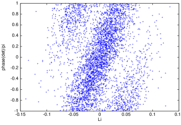
Figure 2: Same as Fig. 1 with $C\approx 1.66$ on a $6^{3}\times 4$ lattice.

3 Constrained Monte Carlo

To test our ideas we developed a HMC algorithm in which the molecular dynamics is forced to evolve on the surface of zero IPPL. This is easily achieved by introducing a Lagrange multiplier which must be computed at each step of the molecular dynamics by solving a non-linear equation, which is the condition that the constraint must be obeyed at each step. It can be shown that the dynamics is reversible and that detailed balance is satisfied. The additional cost in CPU time caused by the constraint is small: 10% more than the unconstrained case for quenched simulations, and completely negligible with dynamical fermions.

As a preliminary test, we made several quenched runs to check the gain of a constrained simulation in comparison with an unconstrained one. We worked with a $4^{3}\times 6$ lattice at $\beta=1.0$ to ensure that we were in the low temperature phase. We got a set of 300 equilibrium quenched configurations and we diagonalized its associated massless staggered fermion matrix, for $\mu=0.5,1.0,1.5$ and $2.0$. Having the eigenvalues of the massless matrix, it is very cheap to get the determinant for any value of the mass.

Let us describe our results. If the mass is large, there is no sign problem in the small and large $\mu$ regions. Simulations are easy but not interesting there. When $\mu$ is of the order $m$ the sign problem becomes severe: this is the region where the onset transition, separating the zero from the finite density phases, takes place. It is very interesting to determine it accurately. Fig. 3a displays $\langle\cos\theta\rangle$ as a function of $m$, for $\mu=1.5$. The logarithmic scale allows us to see the relative error entering Eq. (1). In some cases, the relative error in the unconstrained simulation is one order of magnitude larger than in the constrained one. Notice the severe sign problem signaling a transition for $m\sim 1.75$. The transition region is very broad in the unconstrained simulation, and in fact covers most of the finite density region, between saturation (low $m$) and zero density (high $m$). Actually, almost nothing can be inferred about the finite density phase in the unconstrained case. In the constrained simulation, the sign problem occurs in a much narrower window, so that the onset transition as well as the finite density phase could be analysed. From Fig. 3a, we see that $\mu=1.5$ is nearly critical for $m\in[1.75,1.82]$. As expected, the constraint in the IPPL improves the sign problem and makes numerical simulations feasible. Fig. 3b displays the distribution of $\theta/\pi$ for $\mu=1.5$ and $m=1.5$. The difference between the constrained and unconstrained cases is manifest. An extended version of this work has recently appeared [4].

We thank the authors of Ref. [1], especially Doug Toussaint, for making their data available to us. Ph. de F. thanks Mike Creutz for helpful discussions. V.L. acknowledges useful discussions with R. Aloisio, V. Azcoiti and A. Galante.

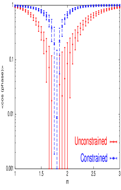
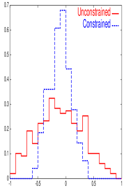
Figure 3: a) Average of $\cos\theta$ vs. fermion mass for $\mu=1.5$; b) Histogram of $\theta/\pi$ for $\mu=1.5$ and $m=1.5$ .

References

- [1] T.C. Blum, J.E. Hetrick, and D. Toussaint, Phys. Rev. Lett. 76 (1996) 1019.
- [2] J. Engels et al., hep-lat/9903030 and these proceedings.
- [3] R. Aloisio et al., Phys. Lett. B453 (1999) 275; hep-lat/9903004.
- [4] Ph. de Forcrand and V. Laliena, hep-lat/9907004.
- [5] K. Langfeld, G. Shin, hep-lat/9907006.