DESY 99-097 HLRZ 99-30 HUB-EP-99/31 FUB-HEP/3-99 TPR-99-09 August 1999 A Lattice Determination of Light Quark Masses

Abstract

A fully non-perturbative lattice determination of the up/down and strange quark masses is given for quenched QCD using both, $O(a)$ improved Wilson fermions and ordinary Wilson fermions. For the strange quark mass with $O(a)$ improved fermions we obtain $m^{\mbox{\tiny$\overline{MS}$}}_{s}(\mu=2\,\mbox{GeV})=105(4)\,\mbox{MeV}$, using the interquark force scale $r_{0}$. Due to quenching problems fits are only possible for quark masses larger than the strange quark mass. If we extrapolate our fits to the up/down quark mass we find for the average mass $m^{\mbox{\tiny$\overline{MS}$}}_{l}(\mu=2\,\mbox{GeV})=4.4(2)\,\mbox{MeV}$.

1 Introduction

Some of the least known parameters in the Standard Model are the light quark masses $m_{u}$, $m_{d}$ and $m_{s}$. Their phenomenological values have been discussed since the early days of the quark model. Paradoxically, the values of the later discovered heavier quarks are more accurately known [1]. The reason is that the connection between light quark masses and observables is highly non-perturbative. This means that the lattice approach is an appropriate technique for this problem.

In this paper we shall present a completely non-perturbative determination of light quark masses. The recent major step forward has been the non-perturbative lattice determination of the renormalisation constants of the mass operators. Also, due to the increase in available computer time, a more reliable continuum extrapolation is now possible.

This paper is organised as follows. In section 2 we discuss the definition of the quark mass and its renormalisation group behaviour. Transcribing lattice data to physical units requires a scale to be set. For quenched QCD this problem is discussed in section 3. The lattice technique for obtaining the quark masses and their renormalisation is presented in section 4. In section 5 we give our results, and in section 6 we extrapolate them to the continuum limit to remove residual discretisation effects. We perform the calculations for both, $O(a)$ improved fermions and for Wilson fermions. Both should extrapolate to the same continuum result, and thus we have a consistency check between the two methods. We have previously used tadpole improved perturbation theory to compute the renormalisation constants. In section 7 we test the validity of this approach. Finally, in section 8 we give our conclusions.

2 Defining the quark mass

Due to confinement quarks are not eigenstates of the QCD Hamiltonian and are thus not directly observable. A definition of the quark mass from an experiment thus means prescribing the measurement procedure. Theoretically this is equivalent to giving a renormalisation scheme ${\cal S}$ and scale $M$. Conventionally, quark masses are given in a mass independent scheme, such as the $\overline{MS}$ scheme, at some given scale $\mu$, commonly taken as $2\,\mbox{GeV}$ [1]. In a general mass independent scheme ${\cal S}$ the renormalised quark mass is given by

$$m^{\cal S}(M)=Z_{m}^{\cal S}(M)m_{bare}.$$ (1)

The running of this renormalised quark mass as the scale $M$ is changed is controlled by the $\beta$ and $\gamma$ functions in the renormalisation group equation. These are defined as scale derivatives of the renormalised coupling and mass renormalisation constant as

$$\beta^{\cal S}\left(g^{\cal S}(M)\right) \equiv \left.{\partial g^{\cal S}(M)\over\partial\log M}\right|_{bare},$$ (2)

$$\gamma_{m}^{\cal S}\left(g^{\cal S}(M)\right) \equiv \left.{\partial\log Z_{m}^{\cal S}(M)\over\partial\log M}\right|_{bare},$$ (3)

where the bare parameters are held constant. These functions are given perturbatively as power series expansions in the coupling constant. The expansion is now known to four loops in the $\overline{MS}$ scheme [2, 3]. We have

$$\beta^{\mbox{\tiny$\overline{MS}$}}(g) = -b_{0}g^{3}-b_{1}g^{5}-b_{2}^{\mbox{\tiny$\overline{MS}$}}g^{7}-b_{3}^{\mbox{\tiny$\overline{MS}$}}g^{9}-\ldots,$$

$$\gamma_{m}^{\mbox{\tiny$\overline{MS}$}}(g) = d_{m0}g^{2}+d_{m1}^{\mbox{\tiny$\overline{MS}$}}g^{4}+d_{m2}^{\mbox{\tiny$\overline{MS}$}}g^{6}+d_{m3}^{\mbox{\tiny$\overline{MS}$}}g^{8}+\ldots,$$ (4)

where (for quenched QCD)

$$\begin{array}[]{lllllll}b_{0}&=&{11\over(4\pi)^{2}},&&b_{1}&=&{102\over(4\pi)^{4}},\\ b_{2}^{\mbox{\tiny$\overline{MS}$}}&=&{1\over(4\pi)^{6}}\left[{2857\over 2}\right],&&b_{3}^{\mbox{\tiny$\overline{MS}$}}&=&{1\over(4\pi)^{8}}\left[{149753\over 6}+3564\zeta_{3}\right],\end{array}$$ (7)

and

$$\begin{array}[]{lllllll}d_{m0}&=&-{8\over(4\pi)^{2}},&&d_{m1}^{\mbox{\tiny$\overline{MS}$}}&=&-{404\over(4\pi)^{4}},\\ d_{m2}^{\mbox{\tiny$\overline{MS}$}}&=&-{2498\over(4\pi)^{6}},&&d_{m3}^{\mbox{\tiny$\overline{MS}$}}&=&-{1\over(4\pi)^{8}}\left[{4603055\over 81}+{271360\over 27}\zeta_{3}-17600\zeta_{5}\right],\end{array}$$ (10)

with $\zeta_{3}=1.20206\ldots$ and $\zeta_{5}=1.03693\ldots$, $\zeta$ being the Riemann zeta function.

We may immediately integrate eq. (2) to obtain

$$M=\Lambda^{\cal S}\left[b_{0}g^{\cal S}(M)^{2}\right]^{b_{1}\over 2b_{0}^{2}}\exp{\left[{1\over 2b_{0}g^{\cal S}(M)^{2}}\right]}\exp{\left\{\int_{0}^{g^{\cal S}(M)}d\xi\left[{1\over\beta^{\cal S}(\xi)}+{1\over b_{0}\xi^{3}}-{b_{1}\over b_{0}^{2}\xi}\right]\right\}}.$$ (11)

The renormalisation group invariant (RGI) quark mass is defined from the renormalised quark mass as

$$m^{RGI}\equiv\Delta Z_{m}^{\cal S}(M)m^{\cal S}(M)=\Delta Z_{m}^{\cal S}(M)Z_{m}^{\cal S}(M)m_{bare},$$ (12)

where

$$[\Delta Z_{m}^{\cal S}(M)]^{-1}=\left[2b_{0}g^{\cal S}(M)^{2}\right]^{d_{m0}\over 2b_{0}}\exp{\left\{\int_{0}^{g^{\cal S}(M)}d\xi\left[{\gamma_{m}^{\cal S}(\xi)\over\beta^{\cal S}(\xi)}+{d_{m0}\over b_{0}\xi}\right]\right\}},$$ (13)

and the integration constant upon integrating eq. (2) is given by $\Lambda^{\cal S}$, and similarly from eq. (3) we have $m^{RGI}$. $\Lambda^{\cal S}$ and $m^{RGI}$ are independent of the scale. Under a change of variable (scheme change or ${\cal S}\to{\cal S}^{\prime}$),

$$g^{{\cal S}^{\prime}}=G(g^{\cal S})=g^{\cal S}(1+c_{1}(g^{\cal S})^{2}+\ldots).$$ (14)

It can be shown that the first two coefficients of the $\beta$ function, the first coefficient of the $\gamma$ function and $m^{RGI}$ are independent of the scheme, while $\Lambda$ only changes as $\Lambda^{{\cal S}^{\prime}}=\Lambda^{\cal S}\exp(c_{1}/b_{0})$.

For the $\overline{MS}$ scheme computing $[\Delta Z_{m}^{\mbox{\tiny$\overline{MS}$}}(\mu)]^{-1}$ involves first solving eq. (11) for $g^{\mbox{\tiny$\overline{MS}$}}(\mu)$ and then evaluating eq. (13). This gives Fig. 1.

Figure 1: One-, two-, three- and four-loop results for $[\Delta Z_{m}^{\mbox{\tiny$\overline{MS}$}}(\mu)]^{-1}$ in units of $\Lambda^{\mbox{\tiny$\overline{MS}$}}$.

We expand the $\beta$ and $\gamma$ functions to the appropriate order and then numerically evaluate the integrals. At $\mu=2\,\mbox{GeV}$ we have $\mu/\Lambda^{\mbox{\tiny$\overline{MS}$}}\sim 8$, and it seems that already at this value we have a fast converging series in loop orders. Indeed, only going from one loop to two loops gives a significant change in $[\Delta Z_{m}^{\mbox{\tiny$\overline{MS}$}}(8\Lambda^{\mbox{\tiny$\overline{MS}$}})]^{-1}$ of order $7\%$. From two loops to three loops we have about $2\%$. The difference between the three-loop and four-loop results is $O(0.5\%)$. So if we are given $m^{RGI}$, and we wish to find the quark mass in the $\overline{MS}$ scheme at a certain scale, we need only use the four-loop result from eq. (13) or equivalently Fig. 1.

3 Digression: which scale to use?

We always need one (or more) experimental numbers as input to set the scale. Ideally, it should not matter what quantity we use. Obvious choices are the force scale $r_{0}$ [4], or the string tension $\sqrt{\sigma}$, or some particle mass (e.g. the proton, or for quenched QCD at least, the $\rho$). So a first requirement is that whatever quantity we use, we should be in a region where the scaling to the continuum limit is the same for all quantities. Thus for $r_{0}$ and the string tension we wish that

$${r_{0}\over a}(g_{0})\times(a\sqrt{\sigma})(g_{0})=\mbox{const}.$$ (15)

over the $g_{0}^{2}\equiv 6/\beta$ region used in the simulations, and indeed for all smaller $g_{0}^{2}$. (We know that this must break down below a value of $\beta$ around $5.7$, due to the appearance of non-universal terms.) In Fig. 2 we show this product.

Figure 2: The product of $r_{0}/a$ and the string tension $a\sqrt{\sigma}$. $(r_{0}/a)(g_{0})$ is taken from the formula given in [5], while the string tension is taken from [6] ($\beta=$ $5.7$, $5.8$, $5.9$, $6.4$), [7] ($\beta=$ $6.0$, $6.2$), [8] ($\beta=6.4$), [9] ($\beta=6.6$).

This seems reasonably constant, with a fit value of $1.170(5)$.

The second requirement is to set the scale in MeV. As we are considering quenched QCD, it is not obvious that choosing scales from different experimental (or phenomenological) quantities will necessarily lead to the same results. Indeed, in the real world [4, 10] the values are

$$r_{0} = 0.5\,\mbox{fm}\equiv(394.6\,\mbox{MeV})^{-1},$$

$$\sqrt{\sigma} = 427\,\mbox{MeV},$$ (16)

($1\,\mbox{fm}^{-1}=197.3\,\mbox{MeV}$) which gives for the product a value of $1.082$ – almost a $10\%$ difference from the quenched value. As both phenomenological estimates come from the same potential model [11], presumably the quenched lattice potential has a slightly different shape from the continuum potential.

Recently, the ALPHA collaboration has determined a value for $\Lambda^{\mbox{\tiny$\overline{MS}$}}$ [12] of

$$\Lambda^{\mbox{\tiny$\overline{MS}$}}=0.602(48)/r_{0},$$ (17)

which may easily be converted using eq. (15) to the string tension scale. However, the numerical value will then suffer from the same $10\%$ ambiguity. Thus we find

$$\Lambda^{\mbox{\tiny$\overline{MS}$}}_{r_{0}} = 238(19)\,\mbox{MeV},$$

$$\Lambda^{\mbox{\tiny$\overline{MS}$}}_{\sqrt{\sigma}} = 220(18)\,\mbox{MeV}.$$ (18)

Our recent spectrum results [13], using $O(a)$ improved fermions, also show a difference whether one uses the $\rho$ or the proton mass to set the scale. Using $r_{0}$ to set the scale is roughly equivalent to using $m_{\rho}$.

In the following we shall adopt the $r_{0}$ scale as given in [5], namely

$$\ln(a/r_{0})=-1.6805-1.7139(\beta-6)+0.8155(\beta-6)^{2}-0.6667(\beta-6)^{3}$$ (19)

(with an error of $0.3\%$ increasing to $0.6\%$ for $\beta$ in the range $5.7\leq\beta\leq 6.57$), but delay using a numerical value for this scale for as long as possible. For the standard scale of $\mu=2\,\mbox{GeV}$ this gives, upon solving eqs. (11) and (13) to the appropriate loop order, the results for $[\Delta Z_{m}^{\mbox{\tiny$\overline{MS}$}}(\mu)]^{-1}$ shown in Table 1. For later reference the results for some other $\mu$ values are also given there, together with $\alpha_{s}^{\mbox{\tiny$\overline{MS}$}}(\mu)$.

$\mu$	one-loop	two-loop	three-loop	four-loop
	$[\Delta Z_{m}^{\mbox{\tiny$\overline{MS}$}}(\mu)]^{-1}$
$2.00\,\mbox{GeV}$	$0.760(10)$	$0.704(9)$	$0.718(10)$	$0.721(10)$
$2.12\,\mbox{GeV}$ ($1/a$ at $\beta=6.0$)	$0.752(10)$	$0.697(8)$	$0.711(9)$	$0.714(10)$
$2.90\,\mbox{GeV}$ ($1/a$ at $\beta=6.2$)	$0.716(8)$	$0.667(7)$	$0.677(7)$	$0.679(8)$
$3.85\,\mbox{GeV}$ ($1/a$ at $\beta=6.4$)	$0.689(7)$	$0.644(6)$	$0.652(5)$	$0.653(6)$
	$\alpha_{s}^{\mbox{\tiny$\overline{MS}$}}(\mu)$
$2.00\,\mbox{GeV}$	$0.268(10)$	$0.195(6)$	$0.201(6)$	$0.202(7)$
$2.12\,\mbox{GeV}$ ($1/a$ at $\beta=6.0$)	$0.261(9)$	$0.191(5)$	$0.196(6)$	$0.197(6)$
$2.90\,\mbox{GeV}$ ($1/a$ at $\beta=6.2$)	$0.228(7)$	$0.170(5)$	$0.174(5)$	$0.175(5)$
$3.85\,\mbox{GeV}$ ($1/a$ at $\beta=6.4$)	$0.205(6)$	$0.156(3)$	$0.159(4)$	$0.159(4)$

Table 1: Useful values of $[\Delta Z_{m}^{\mbox{\tiny$\overline{MS}$}}(\mu)]^{-1}$ and $\alpha_{s}^{\mbox{\tiny$\overline{MS}$}}(\mu)\equiv(g^{\mbox{\tiny$\overline{MS}$}}(\mu))^{2}/4\pi$. The errors are a reflection of the error in eq. (17). The values of $1/a$ are found from eq. (19) together with $r_{0}$ from eq. (16).

4 Determining the quark mass

We shall now derive formulae for the quark masses using the conserved vector current (CVC) and the partially conserved conserved axial vector current (PCAC) by assuming Taylor expansions in the bare quark mass for the relevant functions that occur. We distinguish two quark masses. The Ward identities arising from an infinitesimal vector transformation in the partition function lead to a bare quark mass given by

$$am_{q_{i}}\equiv{1\over 2}\left({1\over\kappa_{q_{i}}}-{1\over\kappa_{c}}\right),\qquad i=1,2,$$ (20)

where $\kappa_{q_{i}}$ is the corresponding hopping parameter, and $\kappa_{c}$ is the critical hopping parameter. This is the standard definition of the quark mass. Similarly, for an infinitesimal axial transformation the Ward Identity (WI) or PCAC definition of the quark mass can be written as

$$a\widetilde{m}_{q_{1}}+a\widetilde{m}_{q_{2}} \stackrel{{\scriptstyle t\gg 0}}{{=}} {\langle\partial_{4}{\cal A}_{4}^{q_{1}q_{2}}(t){\cal P}^{q_{1}q_{2};smeared}(0)\rangle\over\langle{\cal P}^{q_{1}q_{2}}(t){\cal P}^{q_{1}q_{2};smeared}(0)\rangle}$$ (21)

$$\equiv -\sinh am_{PS}^{q_{1}q_{2}}{\langle 0|\hat{\cal A}_{4}^{q_{1}q_{2}}|PS\rangle\over\langle 0|\hat{\cal P}^{q_{1}q_{2}}|PS\rangle},$$ (22)

where ${\cal A}$ (${\cal P}$) is the axial vector current (pseudoscalar density). The precise form of ${\cal A}$ and and ${\cal P}$ will be given later for the $O(a)$ improved as well as the Wilson cases. We have summed the operators over their spatial planes. While ${\cal A}(t)$ and ${\cal P}(t)$ should be point operators, to improve the signal ${\cal P}(0)$ is smeared over its spatial plane. To obtain the second equation, we have re-written eq. (21) in a Fock space and then introduced a complete set of states in the usual way. We have then picked out the lowest pseudoscalar ($PS$) or $0^{-+}$ state whose mass we denote by $m_{PS}^{q_{1}q_{2}}$.

Both definitions of the quark mass must be renormalised. In a scheme ${\cal S}$ at scale $M$ we have

$$m_{q_{i}}^{\cal S}(M) = Z_{m}^{\cal S}(M,am_{q_{i}})m_{q_{i}},$$

$$m_{q_{1}}^{\cal S}(M)+m_{q_{2}}^{\cal S}(M) = \widetilde{Z}_{m}^{\cal S}(M,am_{q_{1}},am_{q_{2}})\left(\widetilde{m}_{q_{1}}+\widetilde{m}_{q_{2}}\right).$$ (23)

The Ward identities give $Z_{m}=1/Z_{S}$ (from $CVC$) and $\widetilde{Z}_{m}=Z_{A}/Z_{P}$ (from $PCAC$).

Let us now Taylor expand $\widetilde{m}$ and the pseudoscalar mass $m_{PS}^{q_{1}q_{2}}$ in terms of the bare quark masses $m_{q_{i}}$,

$$\mbox{\small$\frac{1}{2}$}(a\widetilde{m}_{q_{1}}+a\widetilde{m}_{q_{2}})=$$

$$\widetilde{Y}\left[1+\widetilde{c}\mbox{\small$\frac{1}{2}$}(am_{q_{1}}+am_{q_{2}})+\widetilde{d}{(am_{q_{1}})^{2}+(am_{q_{2}})^{2}\over am_{q_{1}}+am_{q_{2}}}+\ldots\right]\mbox{\small$\frac{1}{2}$}(am_{q_{1}}+am_{q_{2}}),$$

$$(am_{PS}^{q_{1}q_{2}})^{2}=$$ (24)

$$Y_{PS}\left[1+c_{PS}\mbox{\small$\frac{1}{2}$}(am_{q_{1}}+am_{q_{2}})+d_{PS}{(am_{q_{1}})^{2}+(am_{q_{2}})^{2}\over am_{q_{1}}+am_{q_{2}}}+\ldots\right]\mbox{\small$\frac{1}{2}$}(am_{q_{1}}+am_{q_{2}}).$$

The functions must be symmetric under interchange of the quarks, i.e. $q_{1}\leftrightarrow q_{2}$. Only at the lowest (first) order in the quark mass is the functional form simply $am_{q_{1}}+am_{q_{2}}$. At the next order both terms, $(am_{q_{1}}+am_{q_{2}})^{2}$ and $(am_{q_{1}})^{2}+(am_{q_{2}})^{2}$ are allowed. Taylor expanding eq. (23) and comparing with eq. (24) gives us

$$\widetilde{Y}={Z^{\cal S}_{m}(M)\over\widetilde{Z}_{m}^{\cal S}(M)}\equiv{Z^{\cal S}_{P}(M)\over Z_{S}^{\cal S}(M)Z_{A}}.$$ (25)

Renormalisation constants which show no explicit quark mass dependence refer to $m_{q_{1}}=m_{q_{2}}=0$.

We shall also Taylor-expand the matrix elements appearing in eq. (22). First we define the bare pseudoscalar decay constant by $\langle 0|{\cal A}^{q_{1}q_{2}}_{4}|PS\rangle=m^{q_{1}q_{2}}_{PS}f^{q_{1}q_{2}}_{PS}$, and similarly we set $\langle 0|{\cal P}^{q_{1}q_{2}}|PS\rangle=-g^{q_{1}q_{2}}_{PS}$. Expanding the decay constants $f^{q_{1},q_{2}}_{PS}$ and $g^{q_{1}q_{2}}_{PS}$ to first order in the quark masses gives

$$\widetilde{d}=d_{PS}\equiv d,$$ (26)

and hence

$${\mbox{\small$\frac{1}{2}$}\left(a\widetilde{m}_{q_{1}}+a\widetilde{m}_{q_{2}}\right)\over(am_{PS}^{q_{1}q_{2}})^{2}}={\widetilde{Y}\over Y_{PS}}\left[1+\left({\widetilde{c}-c_{PS}\over Y_{PS}}\right)(am_{PS}^{q_{1}q_{2}})^{2}+\ldots\right].$$ (27)

Thus, at least to this order, we have a relation between the WI quark masses and the pseudoscalar mass.

Using eq. (23) gives the renormalised quark mass, and we additionally use eq. (12) to re-write this in a RGI form as

$${\mbox{\small$\frac{1}{2}$}(r_{0}m^{RGI}_{q_{1}}+r_{0}m^{RGI}_{q_{2}})\over(r_{0}m^{q_{1}q_{2}}_{PS})^{2}}=c^{*}_{a}+c^{*}_{b}(r_{0}m^{q_{1}q_{2}}_{PS})^{2}+\ldots,$$ (28)

with

$$c^{*}_{a}=\lim_{g_{0}\to 0}c_{a}(g_{0}),\qquad c^{*}_{b}=\lim_{g_{0}\to 0}c_{b}(g_{0}),$$ (29)

and

$$c_{a} = \left[\Delta Z_{m}^{\cal S}(M)\widetilde{Z}_{m}^{\cal S}(M)\right]\times\left[{\widetilde{Y}\over Y_{PS}}\right]\times\left({r_{0}\over a}\right)^{-1},$$

$$c_{b} = \left[\Delta Z_{m}^{\cal S}(M)\widetilde{Z}_{m}^{\cal S}(M)\right]\times\left[{\widetilde{Y}\over Y_{PS}}\right]\times\left[{-c_{PS}\over Y_{PS}}\left({r_{0}\over a}\right)^{-2}\right]\times\left({r_{0}\over a}\right)^{-1}.$$ (30)

Upon taking the continuum limit $g_{0}\to 0$, any scaling violations will show themselves as non-constant $c_{a}$, $c_{b}$ functions. Equation (28) is the main result of this analysis. Given $c^{*}_{a}$, $c^{*}_{b}$ and the pseudoscalar mass, we can then determine the quark masses.

For the $K^{+}$ ($u\bar{s}$) we set $q_{1}=u$, $q_{2}=s$, and for the $K^{0}$ ($d\bar{s}$) we set $q_{1}=d$, $q_{2}=s$. Together with the $\pi^{+}$ ($u\bar{d}$), with $q_{1}=u$, $q_{2}=d$, this gives from eq. (28)

$$r_{0}m^{RGI}_{s} = c^{*}_{a}\left[(r_{0}m_{K^{+}})^{2}+(r_{0}m_{K^{0}})^{2}-(r_{0}m_{\pi^{+}})^{2}\right]+$$

$$\qquad\qquad c^{*}_{b}\left[(r_{0}m_{K^{+}})^{4}+(r_{0}m_{K^{0}})^{4}-(r_{0}m_{\pi^{+}})^{4}\right]+\ldots,$$

$$r_{0}m^{RGI}_{l} = c^{*}_{a}(r_{0}m_{\pi^{+}})^{2}+c^{*}_{b}(r_{0}m_{\pi^{+}})^{4}+\ldots,$$ (31)

where we have defined $m^{RGI}_{l}=(m^{RGI}_{u}+m^{RGI}_{d})/2$, i.e. the average of the $u/d$ quarks. We have ignored any small corrections due to electromagnetic effects.

5 Numerical results

5.1 Pseudoscalar mesons and bare quark masses

For degenerate quark masses from eq. (24) we have

$$a\widetilde{m}_{q} = \widetilde{Y}\left[1+(\widetilde{c}+d)am_{q}+\ldots\right]am_{q},$$

$$(am_{PS})^{2} = Y_{PS}\left[1+(c_{PS}+d)am_{q}+\ldots\right]am_{q},$$ (32)

and

$${a\widetilde{m}_{q}\over(am_{PS})^{2}}={\widetilde{Y}\over Y_{PS}}\left[1+\left({\widetilde{c}-c_{PS}\over Y_{PS}}\right)(am_{PS})^{2}+\ldots\right],$$ (33)

where $m_{PS}\equiv m_{PS}^{qq}$ (i.e. $q_{1}=q_{2}\equiv q$). Equation (33) gives $\widetilde{Y}/Y_{PS}$ for the $c_{a}$ term in eq. (31), but the gradient $(\widetilde{c}-c_{PS})/Y_{PS}$ is not sufficient to give $-c_{PS}/Y_{PS}$ for the $c_{b}$ term. For $O(a)$ improved fermions, associating the mass expansion parameters $b_{A}$, $b_{P}$ and $b_{m}$ [14] with our expansions, we find $\widetilde{c}\equiv-(b_{A}-b_{P})$ and $d\equiv b_{m}$. First order perturbation theory [15] gives $\widetilde{c}\sim 0.001g_{0}^{2}$.  On top of that $\widetilde{c}/c_{PS}=O(a)$, so that the effect of $\widetilde{c}$ can safely be ignored. For Wilson fermions we shall assume that either $\widetilde{c}$ is small in comparison with $c_{PS}$, as above, or that the complete term $c_{b}(r_{0}m_{K})^{2}$ is small when compared with $c_{a}$. As we shall see, little error is introduced by this assumption.

We have computed the pseudoscalar mass $m_{PS}$ and the WI bare quark mass both, for $O(a)$ improved fermions and Wilson fermions. For improved fermions the calculations were done at $\beta=6.0,6.2,6.4$ and $c_{SW}=1.769,1.614,1.526$ [14], respectively, while for Wilson fermions we only did calculations at $\beta=6.0,6.2$. The computational methods used are standard. For the pseudoscalar mass we used the correlation function

$$C(t) = \langle{\cal P}^{smeared}(t){\cal P}^{smeared}(0)\rangle$$ (34)

$$\stackrel{{\scriptstyle t\gg 0}}{{=}} A\left[e^{-m_{PS}t}+e^{-m_{PS}(T-t)}\right],$$

$T$ being the temporal extent of the lattice. To improve the signal, a Jacobi-smeared operator was used, as described in [10]. For Wilson fermions the pseudoscalar meson mass results can also be found in [10]. The $O(a)$ improved results for $m_{PS}$ are given in Table 5 in the Appendix. The various $\kappa$ values used, the lattice size, and the number of configurations generated are also collated there.

For $a\widetilde{m}_{q}$ the ratio of two point correlation functions as given in eq. (21) was used. For $O(a)$ improved fermions, as well as the action, the operators must also be improved:

$${\cal A}_{\mu} = A_{\mu}+c_{A}a\partial_{\mu}P,$$

$${\cal P} = P,$$ (35)

where $A_{\mu}=\overline{q}\gamma_{\mu}\gamma_{5}q$ and $P=\overline{q}\gamma_{5}q$. By choosing the improvement coefficient $c_{A}(g_{0})$ appropriately, the Ward identity can be made exact to $O(a)$. $c_{A}(g_{0})$ is non-perturbatively known [17]. In Table 6 in the Appendix we give our results for $a\widetilde{m}_{q}$.

Let us first discuss $O(a)$ improved fermions. In Fig. 3

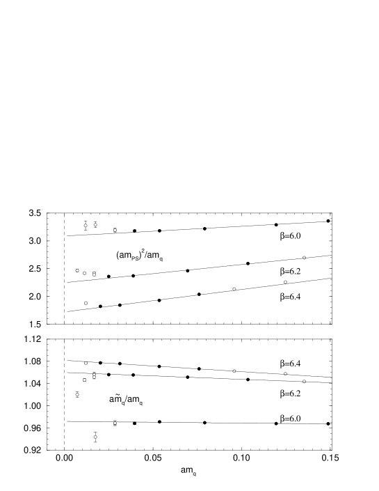
Figure 3: $(am_{PS})^{2}/am_{q}$ and $a\widetilde{m}_{q}/am_{q}$ against $am_{q}$ for $O(a)$ improved fermions. Filled circles denote points used in the fits.

we show the ratios $(am_{PS})^{2}/am_{q}$ and $a\widetilde{m}_{q}/am_{q}$ against $am_{q}$, while in Fig. 4

Figure 4: $a\widetilde{m}_{q}/(am_{PS})^{2}$ against $((r_{0}/a)\times(am_{PS}))^{2}$ for $O(a)$ improved fermions. Filled circles denote points used in the fits. The dashed line ($\sim 3.13$) is $m_{PS}=\sqrt{2}m_{K}$ (which here corresponds to a fictitious $s\overline{s}$ bound state) while the dotted line ($\sim 0.125$) is $m_{\pi}$.

we plot $a\widetilde{m}_{q}/(am_{PS})^{2}$ against $((r_{0}/a)\times(am_{PS}))^{2}$. We must now search for a region where eq. (32), without higher order terms, is valid. For large quark mass values we expect non-linear terms, while for small quark masses quenched QCD chiral logarithms become significant. Finite volume effects do not seem to be a problem, as for $\beta=6.0$, $\kappa=0.1342$ and $\beta=6.2$, $\kappa=0.1352$ we have made runs on two different volumes, without significant changes in the results.

We now make some cuts. In Fig. 4 we see that for small quark masses there are significant deviations from linearity. In particular the light quark mass $m_{l}$ lies in a region where no direct linear extrapolation is possible. However, above $m_{PS}\approx\sqrt{2}m_{K}$ deviations from linearity seem small. We shall thus assume that at least above the strange quark mass any effects of chiral logarithms are small. For heavy quark masses, on the other hand, linearity is still present until at least $m_{q}\approx 3m_{s}\approx\mbox{\small$\frac{1}{3}$}m_{c}$. (Note that $2(r_{0}m_{D})^{2}\sim 44.9$). In this interval lie four or more quark masses. The results of the various fits are given in Table 2.

$\beta$	${\widetilde{Y}\over Y_{PS}}$	${\widetilde{Y}\over Y_{PS}}\times{\widetilde{c}-c_{PS}\over Y_{PS}}\left({r_{0}\over a}\right)^{-2}$	$\widetilde{Y}$
$O(a)$ improved fermions
6.0	0.314(2)	-0.0017(2)	0.972(6)
6.2	0.465(2)	-0.0042(2)	1.060(3)
6.4	0.617(5)	-0.0063(5)	1.082(5)
Wilson fermions
6.0	0.368(4)	-0.00025(51)	0.711(12)
6.2	0.502(6)	-0.0036(5)	0.814(10)

Table 2: Fit values.

For Wilson fermions we simply set ${\cal A}_{\mu}=A_{\mu}$. The results for $a\widetilde{m}_{q}$ have also been given in [10]. In Figs. 5 and 6

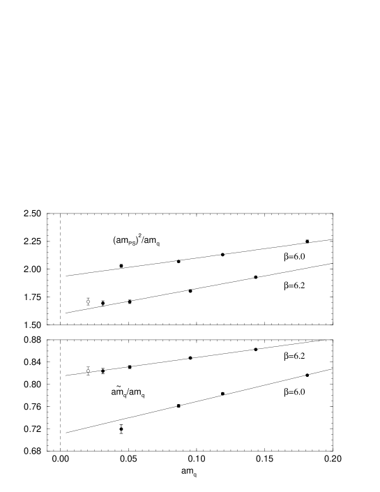
Figure 5: $(am_{PS})^{2}/am_{q}$ and $a\widetilde{m}_{q}/am_{q}$ against $am_{q}$ for Wilson fermions.

Figure 6: The same as Fig. 4 but for Wilson fermions.

we show the ratios $(am_{PS})^{2}/am_{q}$, $a\widetilde{m}_{q}/am_{q}$ and $a\widetilde{m}_{q}/(am_{PS})^{2}$. Similar fit ranges as for improved fermions seem appropriate once more.

To illustrate the $g_{0}^{2}$ dependence of some of these results, we show in Fig. 7

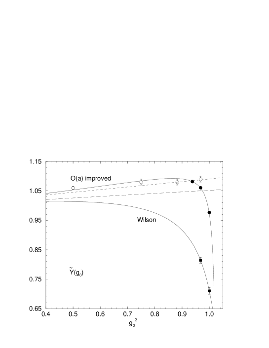
Figure 7: $\widetilde{Y}$ against $g_{0}^{2}$. Our $O(a)$ improved fermion results are shown as filled circles, while those from [16] are shown as open circles. The Wilson fermion results are filled squares. The one-loop perturbation theory results are also shown for the $O(a)$ improved case (dashed line) and the Wilson case (long dashed line).

the results for $\widetilde{Y}$ taken from Table 2 together with Padé-like interpolations of the form

$$\widetilde{Y}(g_{0})={1+p_{1}g_{0}^{2}+p_{2}g_{0}^{4}\over 1+(p_{1}-c)g_{0}^{2}+p_{3}g_{0}^{4}},$$ (36)

arranged so that the perturbative result $\widetilde{Y}(g_{0})=1+cg_{0}^{2}$ with $c=0.09051$ for improved fermions and $0.05195$ for Wilson fermions is obtained for small $g_{0}^{2}$. Possible Padé interpolations are found to be $(p_{1},p_{2},p_{3})=$ $(-1.24,0.256,0.347)$ for $O(a)$ improved fermions and $(-0.944,0.00,0.0746)$ for Wilson fermions. Also shown for comparison are $O(a)$ improved results found in [16]. We see that for $O(a)$ improved fermions first order perturbation theory is good for $g_{0}^{2}\mathrel{\hbox to0.0pt{\lower 4.0pt\hbox{\hskip 1.0pt$\sim$}\hss}\raise 1.0pt\hbox{$<$}}0.96$, while for Wilson fermions a breakdown occurs much earlier.

Thus we now have estimates for $\widetilde{Y}/Y_{PS}$ and $(\widetilde{c}-c_{PS})/Y_{PS}$. $\widetilde{Y}$ will also be needed for Wilson fermions.

5.2 Renormalisation

To compute $c_{a}$ and $c_{b}$ we must now determine the factor $\Delta Z^{\cal S}_{m}(M)Z^{\cal S}_{m}(M)$. For $O(a)$ improved fermions this was done by the ALPHA collaboration [12] using the Schrödinger Functional (SF) method. With the notation of eq. (12) their result can be written as

$$\Delta Z_{m}^{SF}(L^{-1})Z_{m}^{SF}(L^{-1})=1.752+0.321(\beta-6)-0.220(\beta-6)^{2}$$ (37)

(valid for $6.0\leq\beta\leq 6.5$), where they have worked at a scale given in terms of the box size $L$. As emphasised previously, this is a mapping from the bare quark mass to the RGI mass, so this function is the same in all schemes. In eq. (37) the total error is about $2\%$.

For Wilson fermions we use the method proposed in [18] and refined in [19]. This mimics perturbation theory in a certain MOM scheme by considering amputated quark Green’s functions in, say, the Landau gauge, with an appropriate operator insertion. The renormalisation constant is fixed at some scale $p^{2}$. This gives a non-perturbative determination of $Z_{S}^{\mbox{\tiny$MOM$}}(p)$. ($Z_{P}^{\mbox{\tiny$MOM$}}(p)$ is not suitable, as chiral symmetry breaking means that $Z^{\mbox{\tiny$MOM$}}_{P}\to 0$ as we approach the chiral limit, as recently emphasised in [20].) More details of the method, our momentum source approach, and results are given in [19]. As $\Delta Z^{\mbox{\tiny$\overline{MS}$}}_{m}$ is known in the $\overline{MS}$ scheme at scale $\mu$ (see Fig. 1 and Table 1), we can write

$$\Delta Z_{m}^{\mbox{\tiny$MOM$}}(p)\widetilde{Z}_{m}^{\mbox{\tiny$MOM$}}(p)={\Delta Z_{m}^{\mbox{\tiny$\overline{MS}$}}(\mu)\over Z_{S}^{\mbox{\tiny$\overline{MS}$}}(\mu)\widetilde{Y}}\equiv F(\beta),$$ (38)

where we have used eq. (25) and the definitions $Z_{m}=1/Z_{S}$, $\Delta Z_{m}=1/\Delta Z_{S}$ and

$$Z_{S}^{\mbox{\tiny$\overline{MS}$}}(\mu)=X_{S;\mbox{\tiny$MOM$}}^{\phantom{S;}\mbox{\tiny$\overline{MS}$}}(\mu,p)Z_{S}^{\mbox{\tiny$\overline{MS}$}}(p),$$ (39)

with

$$X_{S;\mbox{\tiny$MOM$}}^{\phantom{S;}\mbox{\tiny$\overline{MS}$}}(\mu,p)={\Delta Z_{S}^{\mbox{\tiny$MOM$}}(p)\over\Delta Z_{S}^{\mbox{\tiny$\overline{MS}$}}(\mu)}.$$ (40)

Here $X$ converts the renormalisation constant from the MOM scheme to the $\overline{MS}$ scheme and can be calculated using a continuum regularisation (e.g. naive dimensional regularisation). So we can write

$$X_{S;\mbox{\tiny$MOM$}}^{\phantom{S;}\mbox{\tiny$\overline{MS}$}}(\mu,\mu) = {Z_{S}^{\mbox{\tiny$\overline{MS}$}}(\mu)\over Z_{S}^{\mbox{\tiny$MOM$}}(\mu)}$$ (41)

$$= 1+{\alpha_{s}^{\mbox{\tiny$\overline{MS}$}}(\mu)\over 4\pi}B_{1}+\left({\alpha_{s}^{\mbox{\tiny$\overline{MS}$}}(\mu)\over 4\pi}\right)^{2}B_{2}+\ldots,$$

with $B_{1}=16/3$ [10]. The coefficient $B_{2}$ has recently been calculated [21], giving in the Landau gauge for $N_{f}=0$ flavours a value of $177.48452$. Hence, knowing the coefficients $B_{1}$, $B_{2}$, we can trace back to the more general expression for $X$. A suitable formula is

$$[X_{S;\mbox{\tiny$MOM$}}^{\phantom{S;}\mbox{\tiny$\overline{MS}$}}(\mu,p)]^{-1}=$$ (42)

$$\exp{\left[\int^{g^{\mbox{\tiny$\overline{MS}$}}(\mu)}_{g^{\mbox{\tiny$\overline{MS}$}}(p)}d\xi{\gamma_{m}^{\mbox{\tiny$\overline{MS}$}}(\xi)\over\beta^{\mbox{\tiny$\overline{MS}$}}(\xi)}+\int^{g^{\mbox{\tiny$\overline{MS}$}}(p)}_{0}d\xi\left({\gamma_{m}^{\mbox{\tiny$\overline{MS}$}}(\xi)-\gamma_{m}^{\mbox{\tiny$MOM$}}(G(\xi))\over\beta^{\mbox{\tiny$\overline{MS}$}}(\xi)}\right)\right]},$$

($g^{\mbox{\tiny$MOM$}}=G(g^{\mbox{\tiny$\overline{MS}$}})$ from eq. (14)). Armed with this estimate for $X$, then from eq. (39) we see that $Z^{\mbox{\tiny$\overline{MS}$}}_{S}(\mu)$ should be independent of $p^{2}$, so plotting $Z^{\mbox{\tiny$\overline{MS}$}}_{S}(\mu)$ against $p^{2}$ we expect to see a plateau. In Fig. 8 we show this,

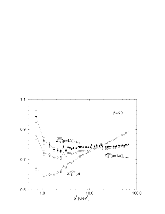
Figure 8: $Z^{\mbox{\tiny$\overline{MS}$}}_{S}(\mu=1/a)$ against $p^{2}$ for $\beta=6.0$. (See [19] for details.) The open squares are the original data, in the chiral limit, while the filled circles represent the results of multiplying $Z^{\mbox{\tiny$MOM$}}(p)$ by $X$ using both coefficients $B_{1}$ and $B_{2}$. The open circles are the result of using only the $B_{1}$ coefficient. The straight line is a fit to the plateau, the length denoting the fit range chosen.

plotting first the original data, extrapolated to the chiral limit, then the results for $Z^{\mbox{\tiny$\overline{MS}$}}_{S}$ when only using $B_{1}$, and finally using both $B_{1}$ and $B_{2}$. We see the data for $Z_{S}$ becoming flatter. The results of the fit are given in the first column of Table 3. The appropriate values for $\widetilde{Y}$ (see Table 2) and $\Delta Z^{\mbox{\tiny$\overline{MS}$}}_{m}(\mu=1/a)$ (see Table 1) are substituted in eq. (38) to give the results listed in the second column of this table.

$\beta$	$Z_{S}^{\mbox{\tiny$\overline{MS}$}}(\mu=1/a)$	$\Delta Z_{m}^{\mbox{\tiny$MOM$}}(p)\widetilde{Z}_{m}^{\mbox{\tiny$MOM$}}(p)$
6.0	0.790(5)	2.49(6)
6.2	0.803(5)	2.25(4)

Table 3: Fit values for the Wilson renormalisation constants.

6 Continuum results

Plotting $c_{a}$ and $c_{b}$ against $a^{2}$ for $O(a)$ improved fermions, and against $a$ for Wilson fermions, we can now extrapolate these coefficients to the continuum limit. In Fig. 9

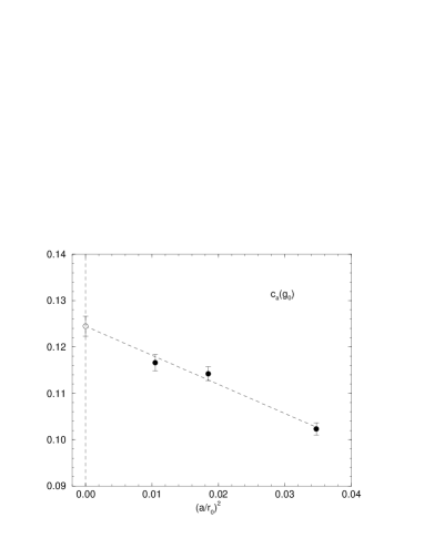
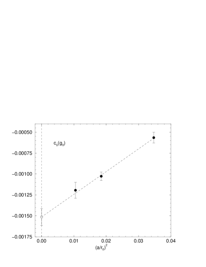
Figure 9: The continuum extrapolation for $c_{a}$ and $c_{b}$ for $O(a)$ improved fermions.

we show the results for $c_{a}$ and $c_{b}$ for improved fermions. A linear fit is also plotted. The results of this fit are given in Table 4. As anticipated, using the first order perturbative result from [15] for $\widetilde{c}$ in $c_{b}$ has no influence on the result.  In Fig. 10 we show the equivalent results for Wilson fermions.

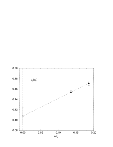
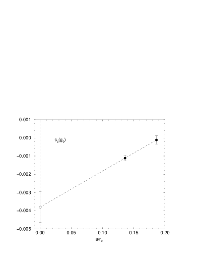
Figure 10: The continuum extrapolation for $c_{a}$ and $c_{b}$ for Wilson fermions.

In this case, as we only have two $\beta$ values, the fit degenerates to an extrapolation. The results of this extrapolation are also given in Table 4. We note that the results for $O(a)$ improved fermions and Wilson fermions for $c_{a}^{*}$ are compatible with each other.

	$c_{a}^{*}$	$c_{b}^{*}$
$O(a)$ improved	0.124(2)	-0.0015(1)
Wilson	0.107(17)	-0.0038(9)

Table 4: The continuum extrapolation of $c_{a}\to c_{a}^{*}$ and $c_{b}\to c_{b}^{*}$ for $O(a)$ improved fermions and Wilson fermions.

Upon inserting these numbers in eq. (31), we find our estimate for the RGI strange and $u/d$ quark masses. To convert to physical numbers, we now have in quenched QCD the uncertainty in the scale, as discussed in section  3. If we use the scale $r_{0}=0.5\,\mbox{fm}$, eq. (16), then together with the experimental values of the $\pi$ and $K$ masses, namely $m_{\pi^{+}}=139.6\,\mbox{MeV}$ and $m_{K^{+}}=493.7\,\mbox{MeV}$, $m_{K^{0}}=497.7\,\mbox{MeV}$, we find the results for $O(a)$ improved fermions

$$m_{s}^{RGI} = 146(4)\,\mbox{MeV},$$

$$m_{l}^{RGI} = 6.1(2)\,\,\mbox{MeV}.$$ (43)

The error comes from Table 4 and from eq. (37). As can also be seen from Table 4, most of the result comes from the constant term, with the slope giving only a small correction to the answer.

For Wilson fermions we have $m_{s}^{RGI}=121(20)\,\mbox{MeV}$, $m_{l}^{RGI}=5.3(8)\,\mbox{MeV}$. This result is somewhat lower than the $O(a)$ improved numbers. We ascribe this mainly to the fact that we only have two values of $\beta$, which makes a continuum extrapolation more difficult. Also the number of $\kappa$ values used and the size of the data sets are smaller than for $O(a)$ improved fermions. Nevertheless, within a one-standard deviation the results are in agreement.

In the $\overline{MS}$ scheme at the ‘standard’ value of $\mu=2\,\mbox{GeV}$, using the four-loop results from Table 1, we find for $O(a)$ improved fermions

$$m^{\mbox{\tiny$\overline{MS}$}}_{s}(\mu=2\,\mbox{GeV}) = 105(4)\,\mbox{MeV},$$

$$m^{\mbox{\tiny$\overline{MS}$}}_{l}(\mu=2\,\mbox{GeV}) = 4.4(2)\,\,\mbox{MeV}.$$ (44)

The corresponding Wilson results are $m^{\mbox{\tiny$\overline{MS}$}}_{s}(\mu=2\,\mbox{GeV})=87(15)\,\mbox{MeV}$ and $m^{\mbox{\tiny$\overline{MS}$}}_{l}(\mu=2\,\mbox{GeV})=3.8(6)\,\mbox{MeV}$.

Note that for the $m_{l}$ quark mass result we have simply extrapolated the fits for the strange quark mass result downwards. The mass ratio $m_{s}/m_{l}$ for $O(a)$ improved fermions is $\approx 23.9$, which is very close to the value given in leading order chiral perturbation theory – namely $(m_{K^{+}}^{2}+m_{K^{0}}^{2}-m_{\pi^{+}}^{2})/m_{\pi^{+}}^{2}\approx 24.2$ (see eq. (31)). This is simply because $|c_{b}^{*}|\ll|c_{a}^{*}|/(r_{0}m_{K})^{2}$, and so the second term in eq. (31) is almost negligible. The mass ratio is then independent of $c_{a}^{*}$.

In Fig. 11 we plot our results.

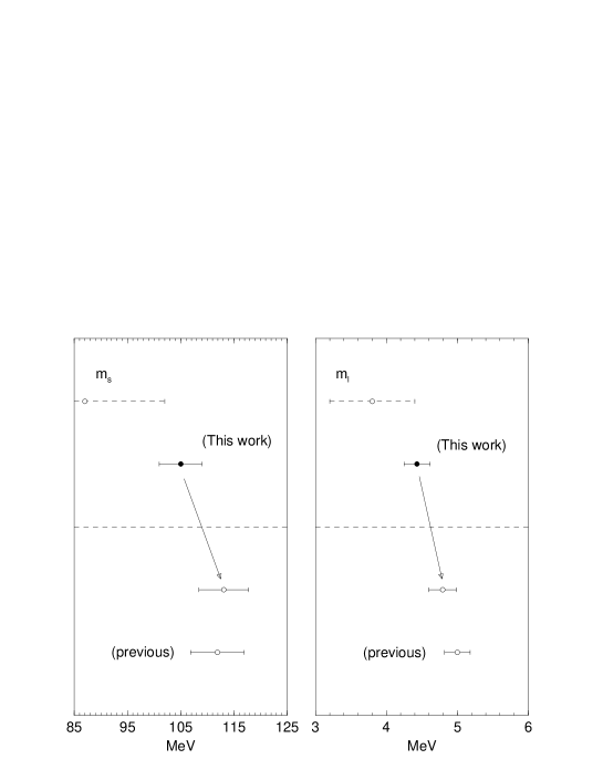
Figure 11: The strange and light quark masses from eq. (44) (‘This work’). The Wilson fermion results are shown dotted. Also shown is our previous result (‘previous’) [10]. The arrows denote the result when using $\sqrt{\sigma}$ as a scale.

Below the dotted line, we have given our previous result [10], using the string tension as the scale, as given in eq. (16). As a comparison we have also re-plotted our result given in eq. (44) using $\sqrt{\sigma}$ as the scale. A reasonable agreement is seen. As our previous result used tadpole improved (TI) perturbation theory to determine the renormalisation constant, it would seem that the use of TI perturbation theory does not introduce much error. In the next section we shall briefly investigate this point.

7 Digression: comparison with tadpole-improved perturbation theory

In this section we shall discuss how reliable TI perturbation theory is. Lowest order perturbation theory gives

$$Z_{S}^{\mbox{\tiny$\overline{MS}$}}(\mu=1/a)=1-{g_{0}^{2}\over 16\pi^{2}}C_{F}B^{\mbox{\tiny$\overline{MS}$}}(c_{SW})+O(g_{0}^{4}).$$ (45)

The $B$ coefficient is uncomfortably large [10]. In [22] this was traced to large tadpole diagrams in the perturbation expansion and also to the expansion in a non-physical (bare) coupling constant. Removing the tapole diagrams and expanding in (say) $\alpha_{s}^{\mbox{\tiny$\overline{MS}$}}$ gives the improved series

$$Z_{S}^{\mbox{\tiny$\overline{MS}$}}(\mu=1/a)=u_{0}\left(1-{\alpha_{s}^{\mbox{\tiny$\overline{MS}$}}(\mu=1/a)\over 4\pi}C_{F}\left[B^{\mbox{\tiny$\overline{MS}$}}(\widetilde{c}_{SW})-\pi^{2}\right]\right)+O(\alpha_{s}^{2}),$$ (46)

with $u_{0}=\langle\mbox{\small$\frac{1}{3}$}\mbox{Tr}U_{plaq}\rangle^{\mbox{\small$\frac{1}{4}$}}$ to be numerically determined, and $\widetilde{c}_{SW}=c_{SW}u_{0}^{3}$. A description of our variation of this procedure is given in [10]. In particular, we choose $c_{SW}$ to be the non-perturbatively determined result, rather than setting it to be equal to $1/u_{0}^{3}$. $\alpha_{s}^{\overline{MS}}$ corresponds to the four-loop results (see Table 1) also used in [22].

As we now have a genuine non-perturbative determination of $Z_{m}$ available, it is of interest to compare how the different results scale to the continuum limit. It is convenient to first define for two $O(a)$ improved estimations of the renormalisation constant the ratio

$$R={\Delta Z^{{\cal S}_{1}}_{m}(M_{1})Z_{m}^{{\cal S}_{1}}(M_{1})\over\Delta Z^{{\cal S}_{2}}_{m}(M_{2})Z_{m}^{{\cal S}_{2}}(M_{2})}=1+O(a^{2}).$$ (47)

For ${\cal S}_{2}$ we choose the SF scheme and the result given in eq. (37), while for ${\cal S}_{1}$ we use the $\overline{MS}$ scheme, together with either the perturbative result, eq. (45), or the $TI$ result, eq. (46).

In Fig. 12 we show the results for the ratio $R$

Figure 12: The results for the ratio $R$ as defined in eq. (47). $Z_{m}^{\overline{MS}}$ has been determined from eq. (45) or eq. (46) and $\Delta Z_{m}^{\mbox{\tiny$\overline{MS}$}}$ taken from Table 1. A simple interpolation has been used between the $\beta$ values. The dot-dashed vertical lines correspond to $\beta=6.0$, $6.2$, $6.4$, from right to left.

for perturbation theory and TI perturbation theory, using consistently the one-, two- and four-loop results from Table 1. As we originally used one-loop perturbation theory results, it seems more consistent to also use the one-loop result for $\Delta Z_{m}$ when converting $Z^{\overline{MS}}_{S}$ to the $RGI$ result. This gives the solid line in the figure. This was the approach adopted in [10]. We expect $O(a)$ effects to become apparent as $a^{2}\to 0$ if ${\cal S}_{1}$ is not exactly $O(a)$ improved. However, a linear fit in $a^{2}$ for the TI result (with one-loop $\Delta Z_{m}$) appears to go to $R=1$ with an error of only about $2\%$, while for the equivalent perturbative result the error is about $10\%$. Thus, in this case tadpole improving the perturbative result does give better results. However, choosing other loop orders changes the picture somewhat and can make using perturbation theory a better choice. We would like to emphasise that this picture does not have to hold for other renormalisation constants. Strictly speaking a case-by-case analysis is required.

8 Conclusions

In this article we have calculated the strange and $u/d$ quark masses for quenched QCD, both for $O(a)$ improved fermions and Wilson fermions, using a non-perturbatively determined renormalisation constant. Our results are given in eq. (44) and the lines that follow it. Corrections to leading order chiral perturbation theory are small, if we stay away from the region where chiral logarithms become significant. We have also seen that using TI perturbation theory rather than simple perturbation theory does not automatically lead to an improvement of the continuum result.

Note added

While this work was being completed, we received a copy of [23]. This contains some similar results to ours.

Appendix

In Table 5 we give our parameter values used in the $O(a)$ improved fermion simulations together with the measured pseudoscalar mass. For most of the overlapping values with [10] there has been some increase in statistics.

$\beta$	$c_{sw}$	$\kappa$	Volume	$\#$ configs.	$am_{PS}$
6.0	1.769	0.1217	$16^{3}\times 32$	$O(150)$	1.2546(12)
6.0	1.769	0.1263	$16^{3}\times 32$	$O(150)$	0.9704(11)
6.0	1.769	0.1285	$16^{3}\times 32$	$O(150)$	0.8189(11)
6.0	1.769	0.1300	$16^{3}\times 32$	$O(160)$	0.7071(16)
6.0	1.769	0.1310	$16^{3}\times 32$	$O(160)$	0.6268(16)
6.0	1.769	0.1324	$16^{3}\times 32$	$O(990)$	0.5042(7)
6.0	1.769	0.1333	$16^{3}\times 32$	$O(990)$	0.4122(9)
6.0	1.769	0.1338	$16^{3}\times 32$	$O(520)$	0.3549(12)
6.0	1.769	0.1342	$16^{3}\times 32$	$O(1300)$	0.3012(10)
6.0	1.769	0.1342	$24^{3}\times 32$	$O(200)$	0.3017(13)
6.0	1.769	0.1346	$24^{3}\times 32$	$O(200)$	0.2390(12)
6.0	1.769	0.1348	$24^{3}\times 32$	$O(200)$	0.1978(16)
6.2	1.614	0.1247	$24^{3}\times 48$	$O(100)$	1.0284(9)
6.2	1.614	0.1294	$24^{3}\times 48$	$O(100)$	0.7217(9)
6.2	1.614	0.1310	$24^{3}\times 48$	$O(100)$	0.6043(9)
6.2	1.614	0.1321	$24^{3}\times 48$	$O(260)$	0.5183(6)
6.2	1.614	0.1333	$24^{3}\times 48$	$O(560)$	0.4136(6)
6.2	1.614	0.1344	$24^{3}\times 48$	$O(560)$	0.3034(6)
6.2	1.614	0.1349	$24^{3}\times 48$	$O(560)$	0.2431(7)
6.2	1.614	0.1352	$24^{3}\times 48$	$O(260)$	0.2016(10)
6.2	1.614	0.1352	$32^{3}\times 64$	$O(110)$	0.2005(9)
6.2	1.614	0.1354	$32^{3}\times 64$	$O(290)$	0.1657(6)
6.2	1.614	0.13555	$32^{3}\times 64$	$O(280)$	0.1339(7)
6.4	1.526	0.1313	$32^{3}\times 48$	$O(100)$	0.5305(9)
6.4	1.526	0.1323	$32^{3}\times 48$	$O(100)$	0.4522(10)
6.4	1.526	0.1330	$32^{3}\times 48$	$O(100)$	0.3935(12)
6.4	1.526	0.1338	$32^{3}\times 48$	$O(200)$	0.3213(8)
6.4	1.526	0.1346	$32^{3}\times 48$	$O(200)$	0.2402(8)
6.4	1.526	0.1350	$32^{3}\times 48$	$O(200)$	0.1923(9)
6.4	1.526	0.1353	$32^{3}\times 64$	$O(260)$	0.1507(8)

Table 5: Parameter values used in the simulations, together with the measured pseudoscalar mass.

The results for the WI quark mass, $a\widetilde{m}_{q}$, are first split into two pieces. $2a\widetilde{m}^{(0)}_{q}$ denotes the mass coming from the $\langle\partial_{4}A_{4}P^{smeared}\rangle/\langle PP^{smeared}\rangle$ ratio, while $2a\widetilde{m}^{(1)}_{q}$ is the result of $\langle\nabla^{2}_{4}PP^{smeared}\rangle/\langle PP^{smeared}\rangle$. The sum $2a\widetilde{m}_{q}=2a\widetilde{m}_{q}^{(0)}+2c_{A}a\widetilde{m}_{q}^{(1)}$ gives the WI quark mass. All these results are given in Table 6. We define $(\partial_{4})_{xy}\equiv(\delta_{x+\hat{4},y}-\delta_{x-\hat{4},y})/2$. $\partial_{4}\partial_{4}$ has been replaced by $(\nabla^{2}_{4})_{x,y}\equiv\delta_{x+\hat{4},y}-2\delta_{x,y}+\delta_{x-\hat{4},y}$. In the continuum limit both $\partial_{4}\partial_{4}$ and $\nabla^{2}_{4}$ give the same derivative. On the lattice we choose the discretisation $\nabla^{2}_{4}$ with the smallest (temporal) extension. In [10] the choice $\partial_{4}\partial_{4}$ was used.

$\beta$	$c_{sw}$	$\kappa$	$2a\widetilde{m}_{q}^{(0)}$	$2a\widetilde{m}_{q}^{(1)}$	$2a\widetilde{m}_{q}$
6.0	1.769	0.1217	0.9677(7)	1.7867(33)	0.8197(5)
6.0	1.769	0.1263	0.5936(4)	1.0173(24)	0.5093(3)
6.0	1.769	0.1285	0.4340(3)	0.7080(22)	0.3754(3)
6.0	1.769	0.1300	0.3314(3)	0.5227(21)	0.2881(3)
6.0	1.769	0.1310	0.2651(3)	0.4072(20)	0.2313(3)
6.0	1.769	0.1324	0.1751(1)	0.2609(8)	0.1535(1)
6.0	1.769	0.1333	0.1186(1)	0.1737(7)	0.1042(1)
6.0	1.769	0.1338	0.08734(21)	0.1274(9)	0.07678(18)
6.0	1.769	0.1342	0.06282(16)	0.09217(62)	0.05519(15)
6.0	1.769	0.1342	0.06294(27)	0.0932(12)	0.05522(25)
6.0	1.769	0.1346	0.03772(32)	0.0584(11)	0.03289(32)
6.0	1.769	0.1348	0.02485(37)	0.0399(12)	0.02154(37)
6.2	1.614	0.1247	0.7342(3)	1.1520(18)	0.6915(2)
6.2	1.614	0.1294	0.4011(2)	0.5451(12)	0.3809(2)
6.2	1.614	0.1310	0.2966(2)	0.3776(10)	0.2826(2)
6.2	1.614	0.1321	0.2272(1)	0.2748(7)	0.2170(1)
6.2	1.614	0.1333	0.15265(5)	0.1741(4)	0.14620(5)
6.2	1.614	0.1344	0.08542(6)	0.09336(36)	0.08196(5)
6.2	1.614	0.1349	0.05510(6)	0.05985(34)	0.05288(6)
6.2	1.614	0.1352	0.03688(11)	0.04073(46)	0.03537(11)
6.2	1.614	0.1352	0.03703(12)	0.04046(37)	0.03553(12)
6.2	1.614	0.1354	0.02478(6)	0.02773(18)	0.02375(6)
6.2	1.614	0.13555	0.01549(8)	0.01802(20)	0.01482(8)
6.4	1.526	0.1313	0.2709(1)	0.2870(9)	0.2637(1)
6.4	1.526	0.1323	0.2090(1)	0.2074(9)	0.2038(1)
6.4	1.526	0.1330	0.1660(1)	0.1567(8)	0.1621(1)
6.4	1.526	0.1338	0.1172(1)	0.1045(4)	0.11461(6)
6.4	1.526	0.1346	0.06882(6)	0.05799(38)	0.06736(6)
6.4	1.526	0.1350	0.04467(7)	0.03739(35)	0.04373(6)
6.4	1.526	0.1353	0.02661(5)	0.02276(22)	0.02603(5)

Table 6: Results for the Ward Identity quark mass $2a\widetilde{m}_{q}$.

References

- [1] Review of Particle Physics, Particle Data Group, C. Caso et al, Eur. Phys. J. C3 (1998) 1.
- [2] T. van Ritbergen, J. A. M. Vermaseren and S. A. Larin, Phys. Lett. B400 (1997) 379, hep-ph/9701390.
- [3] J. A. M. Vermaseren, S. A. Larin and T. van Ritbergen, Phys. Lett. B405 (1997) 327, hep-ph/9703284.
- [4] R. Sommer, Nucl. Phys. B411 (1994) 839.
- [5] M. Guagnelli, R. Sommer and H. Wittig, Nucl. Phys. B535 (1998) 389, hep-lat/9806005.
- [6] G. S. Bali and K. Schilling, Int. J. Mod. Phys. C4 (1993), 1167, hep-lat/9308014.
- [7] G. S. Bali, K. Schilling and A. Wachter, Phys. Rev. D56 (1997) 2566, hep-lat/9703019.
- [8] G. S. Bali and K. Schilling, Phys. Rev. D47 (1993) 661, hep-lat/9208028.
- [9] G. S. Bali, private communication.
- [10] M. Göckeler, R. Horsley, H. Perlt, P. Rakow, G. Schierholz, A. Schiller and P. Stephenson, Phys. Rev. D57 (1998) 5562, hep-lat/9707021.
- [11] E. Eichten, K. Gottfried, T. Kinoshita, K. D. Lane and T. M. Yan, Phys. Rev. D21 (1980) 203.
- [12] S. Capitani, M. Lüscher, R. Sommer and H. Wittig, Nucl. Phys. B544 (1999) 669, hep-lat/9810063.
- [13] D. Pleiter et al., talk at Lattice 1999.
- [14] M. Lüscher, S. Sint, R. Sommer and P. Weisz, Nucl. Phys. B478 (1996) 365, hep-lat/9605038.
- [15] S. Sint and P. Weisz, Nucl. Phys. B502 (1997) 251, hep-lat/9704001.
- [16] G. M. de Divitiis and R. Petronzio, Phys. Lett. B419 (1998) 311, hep-lat/9710071.
- [17] M. Lüscher, S. Sint, R. Sommer, P. Weisz and U. Wolff, Nucl. Phys. B491 (1997) 323, hep-lat/9609035.
- [18] G. Martinelli, C. Pittori, C. T. Sachrajda, M. Testa and A. Vladikas, Nucl. Phys. B445 (1995) 81, hep-lat/9411010.
- [19] M. Göckeler, R. Horsley, H. Oelrich, H. Perlt, D. Petters, P. E. L. Rakow, A. Schäfer, G. Schierholz and A. Schiller Nucl. Phys. B544 (1999) 699, hep-lat/9807044.
- [20] J. Cudell, A. Le Yaouanc and C.Pittori, Phys. Lett. B454 (1999) 105, hep-lat/9810058.
- [21] E. Franco and V. Lubicz, Nucl. Phys. B531 (1998) 641, hep-ph/9803491.
- [22] G. P. Lepage and P. B. Mackenzie, Phys. Rev. D48 (1993) 2250, hep-lat/9209022
- [23] J. Garden, J. Heitger, R. Sommer and H. Wittig, hep-lat/9906013.