Efficiencies and optimization of HMC algorithms in pure gauge theory

Abstract

As a prerequisite to dynamical fermion simulations a detailed study of optimal parameters and scaling behavior is conducted for the quenched Schrödinger functional at fixed renormalized coupling. We compare standard hybrid overrelaxation techniques with local and global hybrid Monte Carlo. Our efficiency measure is designed to be directly relevant for the strong coupling constant as used by the ALPHA collaboration.

The measurements are performed in the framework of the Schrödinger Functional, i.e.

• finite lattice with extent $L^{3}\times T$ (here $T=L$),

• periodic boundary conditions in the spatial directions,

• fixed boundary fields $C$ and $C^{\prime}$ at $x_{0}=0$ and $x_{0}=T$, parametrized by a dimensionless parameter $\eta$ [1],

$${\mathcal{Z}}[C,C^{\prime}]=e^{-\Gamma}=\int[dU]e^{-S[U]}.$$ (1)

We consider a pure SU(3) gauge action,

$$S[U]=\beta\sum_{p}w(p)\left(1-\frac{1}{3}\mbox{Re}\mbox{Tr}U_{p}\right).$$ (2)

A renormalized coupling can be extracted from the response of the free energy to the induced colour-electric background field. There is some freedom in the precise definition of the coupling. We choose one which has turned out to be practical in the ALPHA simulations. This coupling is obtained as an expectation value

$$\frac{1}{\bar{g}^{2}}=k^{-1}\frac{\partial\Gamma}{\partial\eta}=k^{-1}\left\langle\frac{\partial S}{\partial\eta}\right\rangle.$$ (3)

In this finite volume scheme, the running coupling $\bar{g}$ is a function of the box size $L$. We perform our measurements at constant physics, i. e. with $\beta$ tuned such that the coupling of systems with different $L/a$ match, where $a$ is the lattice spacing.

L/a	$\mathbf{\beta}$	$\mathbf{\bar{g}}^{-2}$
4	6.7796	0.476
6	7.1214	0.476
8	7.3632	0.476
10	7.5525	0.476

We consider the following algorithms:

Heatbath/Overrelaxation (HOR).

Each update is composed of one heatbath sweep followed by $N_{or}$ overrelaxation sweeps.

• Overrelaxation: microcanonical reflections in three SU(2) subgroups.

• Heatbath: Cabbibo-Marinari method with random matrices from SU(2) subgroups. SU(2) matrices are generated with the Fabricius-Haan algorithm.

A sweep consists of loops over $x$ and $\mu$. The order of these loops turned out to have a significant influence on the autocorrelation times (with the inner loop over $x$ being in advantage).

Hybrid Monte Carlo (HMC).

The HMC is a member of the family of algorithms which are based on classical dynamics. To this end, one considers a Hamiltonian

$$H[P,U]=\frac{1}{2}\sum_{x,\mu}P_{x,\mu}^{2}+S[U]$$ (4)

with momenta $P_{x\mu}$ conjugate to the link variables. In each update step, momenta are generated with a Gaussian distribution and a reversible discretized trajectory is computed. Discretization errors are corrected by an acceptance step.

Parameters which can be optimized are the trajectory length $\tau$ and the step size $\delta\tau$.

Local Hybrid Monte Carlo (LHMC).

We also consider a local version of the HMC algorithm proposed in [2]. Here one applies the same procedure as for the global HMC algorithm, but for one link while keeping all others fixed. This has some advantages compared to the global HMC:

• The difference in the action accumulated on a trajectory does not contain a volume factor. As a consequence, much greater step sizes sizes are possible without getting poor acceptance rates.

• The staples for a link – which are involved in the computation of the force – have to be computed only once per trajectory, so additional steps on the trajectory are cheap. This point has turned out to be of minor importance, as the optimal parameter set has $\tau/\delta\tau\approx$ 2 – 3.

An advantage compared to the HOR algorithm is that $\Delta S$ is only needed for infinitesimal $\Delta U$. This makes no practical difference for the standard Wilson action considered here, but it is relevant for more complicated actions where terms quadratic in $U$ appear.

The LHMC algorithm cannot be applied to QCD with pseudofermions in a straightforward way, because the computation of the force would then require the inversion of a fermion matrix in each local step. However, for a simulation of a bermion theory with clover term, which we are preparing, it is an attractive candidate for the update of the gauge field [4].

We mention here that for a Wilson action, the leapfrog algorithm for generating a candidate configuration can be replaced by an exact integration of the equations of motion [3]. The method used there makes use of the fact that in the case where subgroups of SU(3) are updated separately, the action takes the form of the energy of a ”pendulum”.

We want to represent efficiency measures in a way that allows a machine-independent comparison of algorithms. Thus, we define a measure $S_{\mbox{cost}}$ such that in order to compute ${\bar{g}}^{2}$ at $1\%$ accuracy, the equivalent in complexity of $S_{\mbox{cost}}$ computations of all staples is required.

The optimization of the three algorithms used in this study is shown in figures 1 - 5.

In the following we investigate how the different algorithms scale with $L/a$. The variance of the coupling between $L/a=4$ and $L/a=10$ behaves approximately like $(L/a)^{1.4}$. Thus, we expect a behaviour of the cost measure $S_{\mbox{cost}}\propto(L/a)^{1.4+z}$. In figure 6 we have plotted $S_{\mbox{cost}}$ with optimized parameters for each algorithm against $L/a$. The dotted lines correspond to exponents $z=1$, $z=2$ resp.

From our data at $L/a=8$ we conclude that typical ratios in $S_{\mbox{cost}}$ for optimized parameters are 1 : 3 : 26 for HOR : LHMC : HMC. This illustrates the cost of HMC even before dynamical quarks are included. A similar performance ratio for HMC and HOR was concluded in [5], which recently came to our attention.

We thank DESY for allocating computer time to this project and the DFG under GK 271 for financial support.

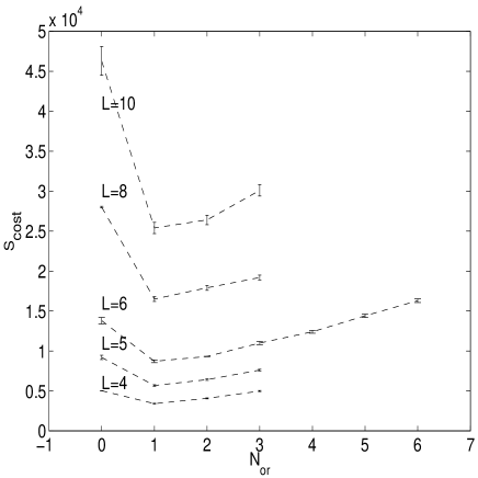
Figure 1: $S_{\mbox{cost}}$ for the HOR algorithm

Figure 2: $S_{\mbox{cost}}$ for global Hybrid Monte Carlo at $L/a=6$. For each data point, the corresponding acceptance is shown.

Figure 3: $S_{\mbox{cost}}$ for global Hybrid Monte Carlo at $L/a=8$.

Figure 4: $S_{\mbox{cost}}$ for Local Hybrid Monte Carlo at $L/a=6$.

Figure 5: $S_{\mbox{cost}}$ for Local Hybrid Monte Carlo at $L/a=8$.

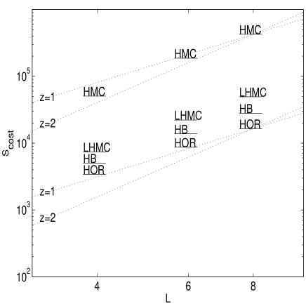
Figure 6: Optimal $S_{\mbox{cost}}$ for the different algorithms in a double-logarithmic representation. For comparison, dotted lines which correspond to exponents $z=1,2$ are displayed. The points denoted with HB correspond to a pure heatbath.

References

- [1] M. Lüscher, R. Sommer, P. Weisz and U. Wolff, Nucl. Phys. B413 (1994) 481. hep-lat/9309005.
- [2] P. Marenzoni, L. Pugnetti and P. Rossi, Phys. Lett. B315 (1993) 152. hep-lat/9306013.
- [3] A. D. Kennedy and K. M. Bitar, Nucl. Phys. Proc. Suppl. 34 (1994) 786-788. hep-lat/9311017.
- [4] J. Rolf and U. Wolff, contribution to these proceedings. hep-lat/9907007.
- [5] R. Gupta, G. Kilcup, A. Patel, S. Sharpe and Ph. de Forcrand, Mod. Phys. Lett. A3 (1988) 1367.