Confinement in QCD

Abstract

The guiding lines of the lattice investigations on colour confinement are reviewed, together with recent results.

1 Introduction

Colour is confined in nature. The experimental upper limit on abundance of quarks $n_{q}$, on abundance of protons $n_{p}$ is

$$\frac{n_{q}}{n_{p}}\leq 10^{-27}$$ (1)

corresponding to Millikan like analysis of $\sim 1g$ of matter. If there were no confinement a conservative expectation in the cosmological standard model would be[1]

$$\frac{n_{q}}{n_{p}}\simeq 10^{-12}$$ (2)

A factor $10^{-15}$ is convincing evidence for confinement. Its smallness also indicates that confinement cannot be explained by fine tuning of a small parameter, but only in terms of symmetry. An analogous situation exists in superconductivity[2]. The persistence of electric currents during years in a superconductor is explained in terms of the change of symmetry of the ground state produced by the Higgs phenomenon. The lifetime of the current is determined by the characteristic correlation time of macroscopic fluctuations.

Confinement must be explained in terms of symmetry and if QCD is the theory of hadrons it should have the relevant symmetry built in.

2 Lattice QCD

QCD most likely exists as a field theory due to asymptotic freedom, in contrast to other field theories like QED, which can only be viewed as effective models, and loose their validity at short distances. In rigorous terms this means that the euclidean Feynman integral which defines the theory

$$Z=\int\left[\prod_{\mu,x}dA_{\mu}(x)\right]\exp(-\beta S)\qquad\beta=\frac{2N_{c}}{g^{2}}$$ (3)

admits a thermodynamical limit.

$Z$ is a functional integral, and is defined as the limit of a sequence of discretized, ordinary integrals. Lattice is an approximant in this sequence, and a good approximation to the limit whenever the correlation length is large compared to lattice spacing, and small compared to the lattice size[3].

Physical quantities computed on the lattice, e.g. by numerical simulations, are therefore determined from first principles. Lattice formulation also defines the correct ground state (vacuum). The usual perturbative quantization in terms of Fock space of gluons and quarks is instead basically ill defined, and the instability of its ground state manifests itself by the existence of singularities (renormalons) in the resummation of the perturbative series[4]. Lattice is therefore specially suited to understand the structure of the theory.

A deep issue in this understanding is the $N_{c}\to\infty$ limit. The idea[5] is that the limit $N_{c}\to\infty$ of QCD, with $\lambda=g^{2}N_{c}$ fixed, defines a field theory, which contains the main physical features of QCD, including confinement of colour. An expansion in $1/N_{c}$, $N_{f}/N_{c}^{2}\ldots$ is well defined and is a correction to the limiting theory. A fermion loop in this expansion is roughly speaking ${\cal O}(N_{f}/N_{c}^{V/2})$ where $V$ is the number of gluon-quark vertices. For $V>2$ this is a small correction, and only the loops with $V=2$ are ${\cal O}(1)$. Quark loops are negligible except for the rescaling of $\Lambda_{Lattt}$ due to contribution of quarks loop with $V=2$ to the $\beta$ function. Numerical simulations on lattice do support this expectation.

An alternative evidence in this direction is the solution of the $U(1)$ problem[6], where the mass of the $\eta^{\prime}$, $m_{\eta^{\prime}}$ is related by $1/N_{c}$ arguments to the topological susceptibility $\chi$ of the quenched QCD vacuum[7]

$$2N_{f}\chi=f_{\pi}^{2}m_{\eta^{\prime}}^{2}$$ (4)

where

$$\chi=\int d^{4}x\langle T(Q(x)Q(0))|0\rangle$$ (5)

$Q(x)$ is the topological charge density, $N_{f}$ the number of light fermions, $f_{\pi}$ the pion decay constant.

Eq.(4) predicts $\chi(180\,{\rm MeV})^{4}$ and this prediction is confirmed by lattice simulations[8].

All this points to the independence of the confinement mechanism on $N_{c}$, $N_{f}$.

The change of symmetry leading to confinement should not depend on $N_{c}$, $N_{f}$.

3 Finite temperature QCD

The standard way to define a static thermodynamics of QCD is to limit the euclidean time direction from 0 to $t_{E}$

$$t_{E}=1/T$$ (6)

with periodic boundary conditions for bosons, antiperiodic for fermions.

In lattice QCD an asymmetric lattice is used $N_{s}^{3}\times N_{t}$, with $N_{s}\gg N_{t}$. At a given value of the lattice unrenormalized coupling $\beta=2N_{c}/g^{2}$ the temperature will be defined by eq.(6) as

$$a(\beta)N_{t}=\frac{1}{T}$$ (7)

in terms of the lattice spacing $a(\beta)$.

The value of $a(\beta)$ in physical units, depends on $\beta$ via renormalization group. At one loop

$$a(\beta)=\frac{1}{\Lambda_{Latt}}\exp(-b_{0}\beta)$$ (8)

where $b_{0}>0$ is the negative of the first coefficient of the perturbative expansion of the $\beta$ function.

At a given $\beta$ then

$$T=\frac{\Lambda_{Latt}}{N_{t}}\exp(b_{0}\beta)$$ (9)

Temperature increases exponentially with $\beta$: the deconfining transition from hadrons to quark gluon plasma will take place at some value of $\beta$. For $T>T_{c}$, or in the weak coupling regime, the order parameter of the theory, the Polyakov line $\langle P\rangle$ is $\neq 0$, and quarks and gluons exist as particles[9]. For $T<T_{c}$, $\langle P\rangle=0$, and there is confinement. In general $\langle P\rangle$ is related to the chemical potential of a single quark, $\gamma$, by the equation

$$\langle P\rangle=\exp(-\gamma)$$ (10)

so that the confined phase corresponds to $\gamma=\infty$: an infinite amount of energy is needed to create an isolated quark. From the point of view of symmetry $T<T_{c}$ is the disordered phase, or the strong coupling regime.

If confinement is due to symmetry, the obvious question is: what is the symmetry of a disordered phase? As we shall see the key word in this respect is “duality”.

Before going to duality we underline two points:

• $\langle P\rangle$ is an order parameter only in the absence of quarks. In view of the $N_{c}\to\infty$ argument presented above, such situation is not satisfactory. A order parameter should exist for the two situations.

• Evidence from lattice exists that confinement takes place in QCD. Below $T_{c}$ the $Q\bar{Q}$ potential $V(R)$, as determined from Wilson loop, is[10]

  $$V(R)=\sigma R\qquad\sigma={\hbox{string tension}}$$ (11)

  Above $T_{c}$ the force is a screened Coulomb force. Moreover in the confined phase the linear potential is related to the existence of chromoelectric flux tubes joining the $Q\bar{Q}$ pair, whose energy is proportional to the length[11, 12]

4 Duality

Duality is a typical property of ($d+1$) dimensional systems which can have spatial ($d$ dimensional) configurations with non-trivial topology and conserved topological charge. At low $g^{2}$ the system is described in terms of local fields $\Phi$, the symmetry is identified in terms of order parameters $\langle\Phi\rangle$ and there is order. At high $g^{2}$, $\langle\Phi\rangle\to 0$, and disorder sets in.

However a dual description exists, in which the extended structures with topology are described by local fields, $\mu$, the original $\Phi$ fields become non local, and the effective coupling constant is $g^{\prime}\sim 1/g^{2}$. In this description the original disordered phase is ordered and viceversa. The dual symmetry is described by $\langle\mu\rangle$ which is called a disorder parameter.

The prototype model of duality is the 2 dimensional Ising model, where the topological configurations are kinks[14].

Other examples are liquid $He_{4}$, with vortices[15], the Heisenberg ferromagnet[16], with non abelian vortices or Weiss domains, and the usual 3+1 dimensional gauge theories, with monopoles. $U(1)$ is an example[17], SUSY QCD[18] is another and finally QCD, as we shall show in what follows.

The strategy that we adopt is to identify the dual symmetry, and to construct the disorder parameter $\langle\mu\rangle$ in terms of the original local fields $\Phi$, which in QCD are gluons and quarks. This strategy is inspired by ref.[19] and has been adapted on lattice by our group. An alternative strategy consist in performing the transformation to dual[14, 13], but is less convenient in numerical investigations.

5 Monopoles in QCD

A guess of the dual symmetry in QCD is that the vacuum in the confined phase is a dual superconductor[20]. The phenomenological motivation is that in a dual superconductor dual Meissner effect will constrain the chromoelectric field acting between a $Q\bar{Q}$ pair into an Abrikosov like flux tube, with energy proportional to the length, or to the distance

$$V(R)=\sigma R$$ (12)

Monopoles are objects with nontrivial topology, when described in terms of the gauge fields. The signal of dual superconductivity should be the nonvanishing of the vacuum expectation value of an operator carrying magnetic charge, the analog of the Ginsburg Landau charged Higgs field in ordinary superconductivity[21].

Monopoles in QCD are well understood[22, 23]. They can be exposed by a procedure known as abelian projection[24]. We shall sketch it for SU(2) gauge fields: the extension to SU(N) is trivial.

To each operator $\Phi(x)\equiv\vec{\Phi}(x)\cdot\frac{\vec{\sigma}}{2}$ in the adjoint representation a gauge transformation $R(x)$ can be associated, which brings $\vec{\Phi}$ parallel to 3 axis, or $\Phi(x)$ to a diagonal $2\times 2$ matrix, proportional to $\sigma_{3}$. $R(x)$ is called “abelian projection” and is defined everywhere except at zeros of $\vec{\Phi}(x)$. We shall define for convenience

$$\hat{\Phi}(x)=\frac{\vec{\Phi}(x)}{|\vec{\Phi}(x)}$$ (13)

The field strength[22]

$$F_{\mu\nu}=\hat{\Phi}\cdot\vec{G}_{\mu\nu}-\frac{1}{g}\hat{\Phi}\cdot(D_{\mu}\hat{\Phi}\wedge D_{\nu}\hat{\Phi})$$ (14)

with $\vec{G}_{\mu\nu}$ the usual field strength and $D_{\mu}=\partial_{\mu}-g\vec{A}_{\mu}\wedge$ the covariant derivative, is a gauge invariant, colour singlet operator. By construction the bilinear term in $A_{\mu}$ cancels between the two terms in eq.(14) and in the abelian projected gauge

$$F_{\mu\nu}=\partial_{\mu}A^{3}_{\nu}-\partial_{\nu}A^{3}_{\mu}$$ (15)

looks like an abelian field. Its dual $F^{*}_{\mu\nu}=\frac{1}{2}\varepsilon_{\mu\nu\rho\sigma}F^{\rho\sigma}$ defines a magnetic current $j^{M}_{\mu}$ as

$$j^{M}_{\mu}=\partial_{\nu}F^{*}_{\mu\nu}$$ (16)

which is identically conserved

$$\partial_{\mu}j^{M}_{\mu}=0$$ (17)

A magnetic, gauge invariant $U(1)$ symmetry is thus associated to each operator $\Phi(x)$ belonging to the adjoint representation.

$j^{M}_{\mu}$ is not trivially zero: monopoles charges can exist at the sites where $\vec{\Phi}(x)=0$, where the abelian projection $R(x)$ is singular[24].

Dual superconductivity will occur when magnetic charges belonging to the above $U(1)$ condense in the vacuum, and the corresponding electric field, i.e. the chromoelectric field parallel to the 3 color axis after abelian projection, will experience dual Meissner effect.

The disorder parameter $\langle\mu\rangle$ describing monopole condensation can be constructed with a technique tested in a variety of known system[15, 16, 17], following the strategy outlined above. We will not go into the details of the construction, for which we refer to[25].

The transition to superconductor is signalled by a sharp negative peak in the plot of the quantity $\rho=\frac{d}{d\beta}\ln\langle\mu\rangle$ versus $\beta$ (or vs T). The peak becomes sharper as the space volume of the system becomes larger. A typical behaviour is shown in fig.(1).                            Figure 1: $\langle\rho\rangle$ vs. $\beta$ for $SU(2)$ gauge theory.
Plaquette projection, lattice $16^{3}\times 4$. A finite size scaling analysis allows to extract the critical indices and the decoupling temperature[25, 15, 16, 17]. Indeed, for dimensional reasons

$$\mu=L_{s}^{d}\Phi(\frac{a}{\lambda},\frac{\lambda}{N_{s}})$$ (18)

where $a$ is the lattice spacing, $\lambda$ is the correlation length, $N_{s}$ the extension of the system. At $\beta_{c}$, $\lambda$ diverges as $\lambda\simeq(\beta_{c}-\beta)^{-\nu}$, with $\nu$ the correlation critical index, and $a/\lambda\ll 1$. In the limit $a/\lambda\to 0$ the scaling law follows for $\rho=\frac{d}{d\beta}\ln\langle\mu\rangle$

$$\frac{\rho}{L_{s}^{1/\nu}}=\Phi(L_{s}^{1/\nu}(\beta_{c}-\beta))$$ (19)

The quality of scaling is shown in fig.2 for $SU(2)$ and in fig.3 for $SU(3)$. Scaling exists only for the proper values of $\beta_{c}$, $\nu$, which can thus be determined.

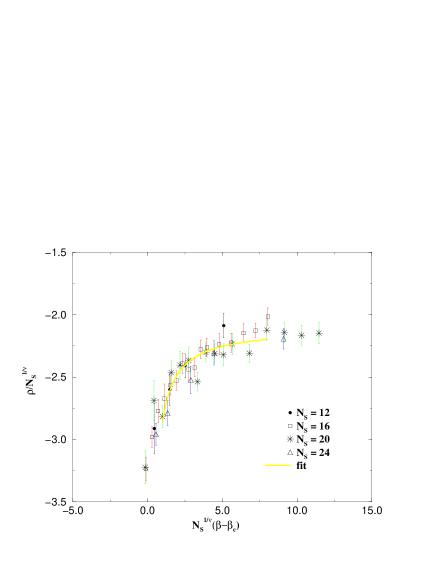
Figure 2: Quality of the scaling for $SU(2)$ gauge theory. Plaquette projection, $N_{t}=4$.

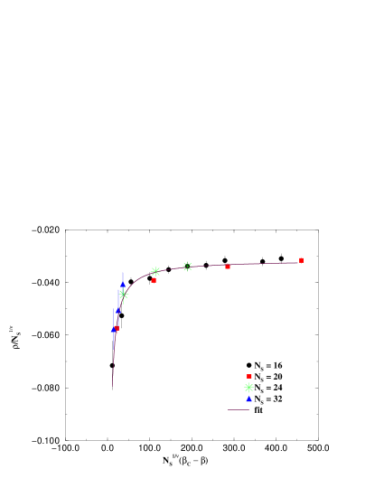
Figure 3: Quality of the scaling for $SU(3)$ gauge theory. Polyakov projection, $N_{t}=4$.

These quantities can also be determined by different methods[9]. They agree within errors. For $SU(2)$ we find

$$\hskip 113.81102pt\begin{array}[]{l}\nu=0.63(5)\\ \beta_{c}=2.30(2)\qquad N_{t}=4\\ \delta=0.20(8)\end{array}\ .$$ (23)

For $SU(3)$

$$\hskip 113.81102pt\begin{array}[]{l}\nu=0.33(2)\\ \beta_{c}=5.70(3)\qquad N_{t}=4\\ \delta=0.54(4)\end{array}\ ,$$ (27)

6 Discussion: open problems.

There is definite evidence that confinement is produced by dual superconductivity. What has not been specified above is the field $\vec{\Phi}(x)$. In principle monopoles exist for any choice of it: a functional infinity of monopoles species. There is no argument a priori that all of them should condense. In ref[24] t’Hooft guesses that all monopoles are physically equivalent, and all of them should condense in the confined phase. What we observe on lattice supports this view. A few choices for $\Phi$ that we have tried look perfectly equivalent.

An alternative attitude exists in the literature, and is that the so called “maximal abelian projection” defines monopoles which are more equal than others. In fact with that choice the abelian field dominates, since after the projection all the fields are oriented in its direction to $90\%$. This choice can be more convenient than others if one looks for effective lagrangians. In principle this convenience does not put any limitation to the symmetry pattern of confinement.

Most probably a better and more syntetic understanding of this symmetry is needed. There must be a reason why all abelian projections are equivalent. However there is no doubt that dual superconductivity is the mechanism of colour confinement.

The part of the work reported due to our group has been done in collaboration with L. Del Debbio, G. Paffuti, P. Pieri, B. Lucini, D. Martelli in the last few years. Their contribution was determinant to the results.

References

- [1] L.B. Okun, Leptons and Quarks, North Holland (1982).
- [2] S. Weinberg, Prog. Theor. Phys., Proc. Suppl. 86 (1986) 43.
- [3] K.G. Wilson, Phis. Rev. D10 (1974) 2445.
- [4] A.H. Müller, Nucl. Phys. B250 (1985) 327.
- [5] G. ’t Hooft, Nucl. Phys. B72 (1974) 461; E. Witten, Nucl. Phys. B160 (1979) 57; P. Di Vecchia, G. Veneziano, Nucl. Phys. B171 (1980) 243.
- [6] S. Weinberg, Phys. Rev. D11 (1975) 3583.
- [7] E. Witten, Nucl. Phys. B156 (1979) 269; G. Veneziano, Nucl. Phys. B159 (1979) 213.
- [8] B. Alles, M. D’Elia, A. Di Giacomo, Nucl. Phys. B494 (1997) 281.
- [9] J. Fringberg, U.M. Heller, F. Karsch, Nucl. Phys. B392 (1993) 493; J.Englert, F. Karsch, K. Redlich, Nucl. Phys. B435 (1995) 295; M. Fukugita, H. Miro,M. Okawa, A. Ukawa, Phys. Rev. Lett. 65 (1990) 816.
- [10] M. Creutz, Phys. Rev. D21 (1980) 2308.
- [11] R.W. Haymaker, J. Wosiek, Phys. Rev. D36 (1987) 3297.
- [12] A. Di Giacomo, M. Maggiore and Š. Olejník, Nucl. Phys. B347 (1990) 441.
- [13] J. Fröhlich, P.A. Marchetti, Commun. Math. Phys. 112 (1987) 343.
- [14] L.P. Kadanoff, H. Ceva, Phys. Rev. B3 (1971) 3918.
- [15] G. Di Cecio, A. Di Giacomo, G. Paffuti, M. Trigiante, Nucl. Phys. B489 (1997) 739.
- [16] A. Di Giacomo, D. Martelli, G. Paffuti, hep-lat/9905007, to appear in Phys. Rev. D.
- [17] A. Di Giacomo, G. Paffuti, Phys. Rev. D56 (1997) 6816.
- [18] W. Seiberg, E. Witten, Nucl. Phys. B431 (1994) 484.
- [19] E. Marino, B. Schroer, J.A. Swieca, Nucl. Phys. B200 (1982) 473.
- [20] S. Mandelstam, Phys. Rep. 23c, 245 (1976); G. ’t Hooft, in “High Energy Physics”, EPS International Conference, Palermo 1975, ed. A. Zichichi.
- [21] A. Di Giacomo, Acta Physica Polonica B25 (1994) 215.
- [22] G. ’t Hooft, Nucl. Phys. B79 (1974) 276.
- [23] A.M. Polyakov, JEPT Letter 20 (1974) 194.
- [24] G. ’t Hooft, Nucl. Phys. B190 (1981) 455.
- [25] A. Di Giacomo, B. Lucini, L. Montesi, G. Paffuti, hep-lat/9906025; A. Di Giacomo, B. Lucini, L. Montesi, G. Paffuti, hep-lat/9906026.